UAG-93: Chapters 1 to 5 - URSI
UAG-93: Chapters 1 to 5 - URSI
UAG-93: Chapters 1 to 5 - URSI

Create successful ePaper yourself
Turn your PDF publications into a flip-book with our unique Google optimized e-Paper software.
t \<br />
I<br />
.(<br />
=<br />
WORLD DATA CENTER A<br />
for<br />
Solar-Terrestrial Physics<br />
\ /-\<br />
) v<br />
IONOGRAM ANALYSIS<br />
WITH THE GENERALISED PROGRAM POLAN<br />
0ecember 1985
YIORL DATA CENTER A<br />
Nat iona I Academy of Sc i ences<br />
2101 Constitution Avenue, NW<br />
Washinq<strong>to</strong>n, D.C. 20418 USA<br />
World Data Center A consists of the Coordination 0ffice<br />
and the fo I lowi nc eioht Subcenters:<br />
COORD I NAT I ON OFF I CE<br />
tlor ld Data Cenier A<br />
National Academy of Sciences<br />
2101 Constifution Avenue, Nl,,l<br />
Washing<strong>to</strong>n, D.C. 20418 USA<br />
lTelephone: (202) 354-3359)<br />
GLACIOLOGY (Snow and |ce)<br />
ROCKETS AND SATELLITES<br />
World Data Center A: Glacioloqy World Data Center A: Rockefs and<br />
(Snow and lce)<br />
Satel I ites<br />
Cooperative Inst. for Research in<br />
Goddard Space Fliqht Center<br />
Env i ronmenta I Sc i ences<br />
Code 60 I<br />
University of Colorado<br />
Greenbelt, Maryland 20771 USA<br />
Boulder, Colorado 80i09 USA Telephone: (l0l) 344-6695<br />
Telephone: (l0l) 492-5111<br />
ROTATION OF THE EARTH<br />
Wor I d Data Center A: Rotat ion<br />
of the Earth<br />
MARINE GEOLOGY AND GEOPHYSICS<br />
U.S. Naval Observa<strong>to</strong>ry<br />
(Gravity, ltlaonetics, Bathymetry,<br />
Washing<strong>to</strong>n, D.C.20590 USA<br />
Seismic Profi les, Marine Sediment, Telephone: (202) 653-i502<br />
and Rock Ana I yses ) :<br />
S0LAR-TERRESTRI AL PHYS I CS ( So lar and<br />
World Daia Center A for Marine<br />
Interplanetary Phencmena, lonospheric<br />
Geology and Geophysics<br />
Phenomena, Flare-Associated Events,<br />
NOAA, E/GC3<br />
Geornagneiic Variations, Aurora,<br />
S75Broadvtay<br />
Cosmic Rays, Airglow):<br />
Bou I der, Co I orado B0J0l USA<br />
Te I ephone: ( l0l) 491-6481 Wor I d Data Center A<br />
for Solar-Terrestrial Phvs ics<br />
N0AA, E/GC2<br />
METEOROLOGY (and Nuclear Radiation)<br />
325 Broadway<br />
World Data Center A: Meteorology Boulder, Colorado B0l0l USA<br />
National Cl imatic Dafa Center Telephone: (303) 491-6323<br />
NOAA, E/CC<br />
Federal Bui lding<br />
S0LID-EARTH GEOPHYSICS (Seismoloqy,<br />
Ashevi I le, North Carol ina 2BB0i USA<br />
Tsunamis, Gravimetry, Earth Tides,<br />
Telephone: (104) 259-0682<br />
Recenf l4ovemenls of the Earthrs<br />
Crust, Magnetic Measuremenis,<br />
Pa I eornagnet i sm and Archeornagnet i sm,<br />
OCEANOGRAPHY<br />
Vo I cano I ogy, Geotherm i cs ) :<br />
World Data Center A: Oceanography<br />
National Oceanographic Data Center<br />
World Data Center A<br />
NOAA, E,/OC<br />
for So I i d-Earth Geophys i cs<br />
2001 Wisconsin Avenue, NW NOAA, E,/GCI<br />
Page Bldg. l, tun. 414<br />
325 Broadway<br />
Washing<strong>to</strong>n, D.C.20235 USA<br />
Boulder, Colorado 80J0J USA<br />
Telephone: (202) 634-7510 Telephone: (l0l) 491-6521<br />
World Data Centers conduct international exchange of geophysical observations in accordance with the<br />
principles set forfh by the lnternational Counci I of Scientific Unions. WDC-A is established in the<br />
United States under the auspices of the National Academy of Sciences. Communicatlons regardinq data<br />
interchange matters in general and World Data Center A as a whole should be addressed <strong>to</strong> Worid Data<br />
Center A, Coordination 0ffice (see address above). lnquiries and co{nmunications concerning dafa in<br />
specific discipl ines should be addressect +^ +ha ia+a su[6snfer I isted above.
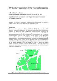
IONOGRAM ANALYSIS t.lITH THE GENERALISED PROGRAM POLAN
450<br />
KAUAI,HA}TAII 09/16/77 0844:43<br />
O-TRACE ONLY<br />
O AND X-TRACES<br />
400<br />
350<br />
a<br />
c 300<br />
F<br />
24n<br />
E 200<br />
150<br />
100<br />
50<br />
1.0 ?.o 3.0 4.0 5.0 6.0 1.0 ?.4 3.0 +.o 5.0 6.0 1.0 2.0 3.0 4.0 5.0 6.0 7.0<br />
FREQUENCY in MHz.<br />
Profiles calculated from digital data obtained with the NOM Dyrasonde.<br />
The program used includes au<strong>to</strong>matic'identificatjon and analysis of sporadic E traces. Enror<br />
boxes at the layer peaks are based on the peak fitting errors returned by P0LAN. The center<br />
curve is the normal analysis in whicn P0LAN selects only those extraordinary ray data which<br />
are useful for start and valley calculations. The right hand curve uses all ordinary and<br />
extraordinary data -- this js not normal ly recommended since differences in echo occurrence.<br />
and horizontal separation o'the rays,.an proouce a oislor!eo profi)e.<br />
Acknowledgements: Some of the work descrjbed in this report was carrted out whije the author<br />
was a guest worker at the N0AA Space Envi r onment Labora<strong>to</strong>ries, BoLrlder, Colorado. I am<br />
grateful <strong>to</strong> Dr. L. F. McNamara for his assistance in the final preparation of this reDorr.<br />
lt
WORLD DATA CENTER A<br />
for<br />
Solar-Terrestrial Physics<br />
REPORT TJAG.<strong>93</strong><br />
ION()GRAM ANALYSIS<br />
WITH THE GENERALISED PROGRAM POLAN<br />
by<br />
J.E. TITHERIDGE<br />
Physics Department<br />
The University of Auckland<br />
Private Bag, Auckland,<br />
New Zealand<br />
December 1985<br />
U.S. DEPARTMENT OF COMMERCE<br />
NATIONAL OCEANIC AND ATMOSPHERIC ADMINISTMTION<br />
NATIONAL ENVIRONMENTAL SATELLITE, OATA Ai/O IIiFORMATION SERVICE<br />
National Geophysical Oata Center<br />
Eoulder- C0 80303 USA
DESCRIPTI0N 0F 'II0RLD DATA CENTERS<br />
orld Data Centers conduct international exchange of geophysical observations in accordance with the principles<br />
set forth by the International Council of Scientific Unions (ICSU). They were established in 1957 by the<br />
International Geophysical Year Con[ittee (CSAGI) as part of the fundarnental international planning for the tGY<br />
prograin <strong>to</strong> collect data fron the nunerous and widespread IGY observationa'l prograns and <strong>to</strong> fiBke such data readily<br />
accessible <strong>to</strong> inlerested scientists and scirolars for an indefinite period of tirn€. liDC-A was established in the<br />
U.S,A.;'iDC-B, in the U.S.S.R.i and IJDC-C, in western Europe, Australia, and Japan. This new syslenr for exchanging<br />
geophysical da<strong>to</strong> was found <strong>to</strong> be very effective, and the operations of the tJorld Data Centers were extended by ICSU<br />
on d continuing basis Lo other interndtional programs; the l,lDC's were under the supervision of the Coitite<br />
lnterndtional de Geophysique (CIG) for the period 1960 <strong>to</strong> 1967 and are now supervised by the ICSU Panel on llJorld<br />
Ddta Centres,<br />
The current plans for continued international exchange of Eeophysical data throuqh the llorld Data Centers are<br />
set forth in lhe Foupth Co4solidated Guide ta Internotional Data Etchange tfu'atgh the l/ot"L,7 |)atta CentTes, issued by<br />
the ICSU Panel on florld Data Centres, These plans are broadly similar <strong>to</strong> those adopted under ICSU auspices for the<br />
IGY dnd subsequent jnternational programs.<br />
I-v-!s!r.9r-:.-q&-R-$p9!:i!i!!$-o-l-tr.qg!<br />
The tlorld Data Centers collect data and pub'ljcations for the following disciplines: Glaciology; i,teteorology;<br />
oceanography; Rockets and Satellites; Solar-Terrestrial Physics disciplines (Solar and lnterp'lanetary Phenonena,<br />
lonospheric Phenomena, Flare Associated Events, Georragnetic Phenornena, Aurora, Cosrnic Rdys, Airglow); Solid-Earth<br />
Geophysics disciplines (Seisnology, Tsunamis, l4ari ne ceologJ and Geophysics, Gravjmetry, Earth Tides, Recenl<br />
r\,lovements of lhe Earth's Crust, Rotation of the Earth, Magnetic Measurements, Paleonagnetism and Archeonagnet i sm,<br />
Volcanology, Geothermics). ln planning for the various scientific prograros, decisions on data exchange viere fiBde<br />
by the scientjfic comnunity through the international scientific unions and comnittees. ln each disciDline the<br />
specialists themselves detennined the nature and form of data exchange, based on their needs as research workers.<br />
Thus the type and amount of data in the WDC'S differ from discipline <strong>to</strong> discipline.<br />
The objects of establishing several tlorld Data Centers for collecting observdtional data were: (l) <strong>to</strong> insure<br />
against loss of data by the catastrophic destructjon of a single center, (2) <strong>to</strong> meet the geographical convenience<br />
of, and provide easy coffmunication for, workers in different parts of the wor'ld. Each l,lDC is responsible for: (1)<br />
endeavoring <strong>to</strong> collect a cornplete sel of data in the field or discipline for which it is responsible, (2) safekeeping<br />
of the incoming data, (3) correct copying and reproduction of data, maintajning adequate standards of<br />
clarity and durability, (4) supplying copies <strong>to</strong> other lllDc's of data not received directly, (5) preparation of catalogs<br />
of all data jn its charge, and (6) making data in the !.|DC's available <strong>to</strong> the scientific corununity. The l,{DC's<br />
conduct their operation at no expense <strong>to</strong> ICSU or <strong>to</strong> the ICSU family of un'ions and comnittees.<br />
llorld Data Center A<br />
llorld Data Center A, for v{hich the National Academy of Sciences through the Geophysics Research Board and its<br />
Comlittee on Data Interchange and Data Centers has over-all responsibility, consists of the WDC-A Coordination<br />
office and seven subcenters at scientific institutions in various parts of the ljnited States. The cRB periodically<br />
reviews the activities of I,{DC-A and has conducted several studies on the effectiveness of the ll,lDc systen. As a<br />
result of these reviews and studies some of the subcenters of {DC-A have been relocated so that thei could 'mre<br />
effectively serve the scientific comunity. The addresses of the WDC-A subcenters and Coordination Office are<br />
given inside the front cover.<br />
The data received by WDC-A have been nEde available <strong>to</strong> the scientific comnunity in various ways: (1) reports<br />
containing data and results of experiments have been compiled, published, and t,'idely distributed; (2) synoptib t-ype<br />
data on cards, microfilm, or tables are avaiiable for use-at Lhe subcenters and for loan <strong>to</strong> scientists; (3) copiei<br />
of data and reports are provided upon request.<br />
IV
TABLE OF COI{TEI{TS<br />
Frontispiece and acknowledgements<br />
ABSTRACT<br />
LIST OF F]GURES AND TABLES<br />
IERMI NOLOGY<br />
Pa ge<br />
1<br />
2<br />
i. INTRODUCTION<br />
2. IONOGRAII ANALYSIS PROCEDURES<br />
2.1 Lamination Methods<br />
2.2 Single Polynomial Methods<br />
2.3 0verlapping Polynomials<br />
2.4 Least-Squares Solutjons<br />
B<br />
B<br />
9<br />
l0<br />
3. SELECTIoN 0F AN N(H) l.tETH0D<br />
3.1 Rapid Estimation of Layer Constants<br />
3.? Calculation of Mono<strong>to</strong>nic Profiles<br />
3.3 Full Calculations<br />
11<br />
11<br />
I2<br />
4. A GEI{EMLISED FORIiIIJLATION<br />
4.1 Outl ine<br />
4.2 The Bas i c Equati ons<br />
4.3 Calculation Procedures<br />
5. THEPROGRAI{<br />
POLAN<br />
5.1<br />
5.2<br />
5.3<br />
5.4<br />
5.5<br />
General Characteristics<br />
The Standard Modes of Analysis<br />
Curve Fi tt i ng Procedures<br />
The Layer Peak<br />
The Simpl ified Program SPOLAN<br />
l3<br />
i3<br />
15<br />
i6<br />
l7<br />
19<br />
2L<br />
22<br />
6.<br />
7.<br />
B.<br />
9.<br />
STARTING PROCEDURES FOR THE ORDINARY RAY<br />
6. 1 0utl ine<br />
6.2 The Methods Used in POLAN<br />
6.3 Daytime Starting l,lodels<br />
6.4 A Night-time Starting Model<br />
VALLEYPROCEDURES<br />
FOR THE ORDINARY MY<br />
7.r<br />
7.2<br />
7.3<br />
7.4<br />
0utl i ne<br />
The Standard Vai 1ey<br />
Addition of Physical Constraints<br />
Val ley Options in POLAN<br />
STARTCALCULATIONS<br />
USING THE EXTMORDINARY RAY<br />
B. i Practical 1y 0btainable Information<br />
8.2 Inclusion of Extraordinary-Ray Data<br />
8.3 The Slab Start in P0LAN<br />
8.4 Physical Constraints and Height Iteration<br />
8.5 The Choice of Scal ing Frequencies<br />
8.6 0ther Start Procedures<br />
VALLEYCALCULATIOI{S<br />
USING THE EXTRAORDINARY RAY<br />
9.1 Introduction<br />
9.2 The Normal Analysis - Calculation of Vali.vl.Jidth<br />
9.3 Calculation of Valley 1,,/idth and Depth<br />
9.4 Resul ts |,li th Test Model lonograms<br />
23<br />
24<br />
25<br />
27<br />
28<br />
28<br />
30<br />
33<br />
36<br />
37<br />
39<br />
41<br />
45<br />
49<br />
53<br />
f,4<br />
56<br />
58
10. USIIIG POTAI{<br />
r0. I Implementation<br />
10.2 P0LAN Input Data<br />
ln ? P0LAN 0utput Data<br />
10. 4 Selection and Scal ing of Data<br />
i0. 5 Selection of a Valuefor START<br />
11. SCALII{G AIID AI{ALYSIS }IITH THE PROGRA}I SCION<br />
11.1 0utl ine<br />
Ll.2 Enteri ng Initial Specif ications<br />
ll.3 Definingthe ionogram Coordinates<br />
ll.4 Scal ingthe Ordinary-Ray Trace<br />
REFEREIICES<br />
APPEIIDIX A. THE ABSOLUTE ACCURACY OF THE CALCULATED PROFILES<br />
A. I Relative accuracies with smooth virtual hei ght curves<br />
4.2 The analysis of irregular profiles<br />
A.3 The effect of errors in the virtual hei ght data<br />
APPEIIDIX B. DEPEI{DEIICE OF THE GROUPREFRACTIVE<br />
INDEX OI{ DIP ANGLE<br />
B. l Va l ue s of group i ndex<br />
8.2 Information obtainable usinqo una i.iy.<br />
8.3 The reduction of inteqratioi errors at hiqh dip angles<br />
APPEIIDIX C. THE EFFECTS OF A VARYINGYROFREQUEIICY<br />
C. I Val ues of gyrofrequencyin the ionosphere<br />
C.2 Changes near reflection<br />
c.3 Retardation in the underlyingreg r on<br />
C.4 Model studies<br />
C.5 The choice of gyrofrequency for the underly.ing regions<br />
APPEIIDIX D. moUP Il,lDEX CALCULATIoNS LIITHIN P0LAN<br />
D.1 Calculation of the vj r tual heiqht coeffjcients - The subrout.ine C0EFIC<br />
q.? Delay in the underlying ionisation - The subroutine REDUCE<br />
D.3 Calculation of the gr"oup r-efract.i ve i ndex - The subroutine GIND<br />
APPEI{DIXE. THE COIISTRUCTIOII OF POLAN<br />
E.1 Logic Flow<br />
E.2 Start and Valley Procecures<br />
E.3 Program Parameters<br />
APPEI{DIX F.<br />
F.1 Themain subroutine P0LAN<br />
F.2 Thesubroutines SffUp, SfLdnf'ani sinvnL<br />
F.3 Thesubroutines C0EFIC. ADJUST and REDUCE<br />
r.{+ tneSubr"outines<br />
PEAK, TRACE, SOLVE, SUMVAL and GIND<br />
F. 5 Theprogram SCI0N<br />
APPEI{DIX G.<br />
G.1 The mainline programPOLRUN<br />
G.2 Standard test data<br />
G.3 Standard results anodiscussion<br />
APPEI{DIXH. THE SI}IPLIFIED PROGRAiI SPOLAN<br />
H.l<br />
H.3<br />
PROGRA}I LISTINGS<br />
STAI{OARD TEST DATAAND RESULTS<br />
Construction<br />
Test Resul ts<br />
Li st i ngs<br />
63<br />
64<br />
67<br />
69<br />
73<br />
74<br />
75<br />
75<br />
77<br />
79<br />
B1<br />
B3<br />
B5<br />
BB<br />
91<br />
<strong>93</strong><br />
96<br />
o7<br />
99<br />
102<br />
I04<br />
108<br />
11i<br />
114<br />
i16<br />
r22<br />
125<br />
128<br />
134<br />
r4i<br />
148<br />
i54<br />
161<br />
163<br />
r67<br />
178<br />
179<br />
183
IOI{OGMII ANALYSIS I{ITH THE GENERALISED PROGRAiI POLAII<br />
by<br />
J. E. TITHERIDGE<br />
Physics Department, The University of Auckland<br />
Auckland, New Zealand<br />
ABSTRACT. Different methods for the real-height analysis of ionograms, and their fields<br />
of application, are surveyed. A flexible new procedure is developed <strong>to</strong> give maximum<br />
accuracy and reliability in an au<strong>to</strong>matic, one-pass analysis. The program P0LAN uses<br />
polynomial real-height sections of any required degree, fitting any number of data<br />
points. By choice of a single parameter (MODE) it can reproduce all current methods from<br />
linear-laminations <strong>to</strong> single or overlapping polynomials. In addition a wide range of<br />
ieast-squares modes are available; these are preferable for most purposes, particularly<br />
with oversampled data (as from digital ionosondes). The mode of analysis changes<br />
au<strong>to</strong>matically within the program <strong>to</strong> give an optimised least-squares calculation in the<br />
start, peak and valiey regions. Physically unacceptable solutions are adjusted by<br />
imposing limits on the profile parameters. The new profile coefficients (and the new<br />
fitting error) are obtained directly and rapidly from the previous solution. This<br />
permits repeated application of the adjustments, as required, and cancellation of any<br />
change if it produces an unacceptably large increase in the virtual-height fitting error.<br />
The information available using combined ordinary and extraordinary ray data<br />
is studied under different conditions. Procedures are developed which can solve the<br />
underlying and valley ambiguities with high accuracy, given suitable data, and which<br />
can detect and reject bad data. Physically reasonable models are incorporated in<strong>to</strong> the<br />
least-squares start and valley calculations. This ensures an acceptable, standardised<br />
form for the profiles in these regions when only ordinary ray data are available. With<br />
good ordinary and extraordinary ray data P0LAN produces the maximum amount of information<br />
which can be obtained about the unobserved regions, and results are almost independent of<br />
the physical models. [,rlith poor or inconsistent data, giving a less well-defined solution,<br />
results become increasingly biased <strong>to</strong>wards the physical model so that acceptable results<br />
are obtai ned under most cond i ti ons.<br />
Many of the techniques used in POLAN are new. Procedures and models developed for<br />
the start, peak and valley regions are described in reasonable detail, along with the<br />
precautions found <strong>to</strong> be necessary for maximum accuracy with extraordinary ray data.<br />
Mathematical procedures for ensuring full accuracy at all dip angles are described jn the<br />
appendices. 0ptimum rules for scaling data are also developed and the practical use of<br />
P0LAN is detailed. Al1 programs are listed in the appendices, along with standard test<br />
data and the corresponding outputs. Copies of the programs are available on magnetic<br />
media from World Data Center A.
SU}IIIARY LIST OF FIGURES AND TABLES<br />
SECTIONS I TO 4<br />
No figures or tables.<br />
SECTION 5 - THEPROGRAIiI<br />
POLAN<br />
TABLEl. Panameters for- the standard modes of analysis<br />
FIGURE 1.<br />
The standard modes of analysis in pOLAN.<br />
TABLE2. Calculation times for each mode of pOLAN.<br />
TABLT3. Fitted heights and weights for each mode.<br />
page 1B<br />
1B<br />
20<br />
20<br />
SECTIOI{ 6 - START CALCULATIOI{S US]NG THE ORDINARY RAY<br />
FIGURE 2. The start extrapolation procedure using ordinary-ray data on1y.<br />
TABLE 4. Model starting heights for the analysis of daytime ionograms.<br />
FIGURE 3. Model starting frequencies (FN) for the analysis of daytime ionograms.<br />
FIGURE 4. Model starting heights for the analysis of night-time ionograms.<br />
23<br />
25<br />
26<br />
27<br />
SECTION 7 - YALLEY CALCULATIOI{S US]NG THE ORD]NARY RAY<br />
FIGURE 5. Possible real-height profiles corresponding <strong>to</strong> the same virtua'l heighr curve.<br />
FIGURE 6. The form and notation of the standard valley.<br />
TABLE 5. Parameters for the standard valley.<br />
FIGURT 7. Profiles formed by the superposition of model chapman layers.<br />
FIGURE B. Results from the anaJysis of dual chapman-layer profiles.<br />
FIGURE 9. Real-height changes due <strong>to</strong> a change in the assumed width of the E/F valley.<br />
29<br />
29<br />
29<br />
32<br />
32<br />
35<br />
SECTIOil B - START CALCULATIOI{S USING EXTRAORDiNARY RAY DATA<br />
FIGURE 10. Parameters for the slab stant profile used with extraordinary ray data.<br />
FIGURE 11. Slab start resul ts at varying fmin.<br />
TABLE 6. Resul ts from the slab-start calculation of Figur"e 12.<br />
FIGURE 12. Analysis of a difficult profile, with the addition of physical constraints.<br />
FIGURE 13. Adustments made by poLAN <strong>to</strong> compensate for bad oara.<br />
TABLE 7. Real height errors obtained using different scaling intervals.<br />
TABLE B. Real height errors obtained with different values of fmin.<br />
FIGURE 14. Virtual heights and gradients at low frequencies.<br />
FIGURE 15. Polynomial start results, for different values of fmin.<br />
TABLE 9. Real-height errons obtained with the porynomial start.<br />
TABLT 10. The X-ray frequency shift used for starting corrections in SpSLAN.<br />
FIGURT 16. Results from the single-point starting correction.in spoLAN.<br />
40<br />
40<br />
43<br />
44<br />
44<br />
47<br />
4B<br />
4B<br />
49<br />
50<br />
5i<br />
52<br />
SECTION 9 - VALLEY CALCULATIONS USING EXTRAORDINARY RAY DATA<br />
FIGURE i7. The shape of the standard val1ey model, for different values of VWIDTH.<br />
FIGURE 18. variations obtained by changing the depth of the model va11ey.<br />
FIGURE 19. Profiles used <strong>to</strong> investigate valJey calculation procedures.<br />
54<br />
57<br />
57
FIGURE 20.<br />
F]GURE 21.<br />
FIGURE 22.<br />
FIGURE 23.<br />
Results from 2-parameter valley ca)culations, at dip angles from 0 <strong>to</strong> 90'. 59<br />
Results at two djfferent valley depths, for dip angles from 0 <strong>to</strong> 9Oo. 59<br />
Changes in real height and fitting error as the assumed val1ey depth varies. 60<br />
The virtual-height fitting error as a function of assumed va1ley depth. 61<br />
SECTION IO - THE USE OF POLAN<br />
FIGURE 24. Scal ing points for a typical daytime ionogram.<br />
FIGURE 25. Regions where the 0-ray trace should not be scaled.<br />
7I<br />
71<br />
SECTION 11 - THE PROGRAIiI SCION FOR DIGITISING DATA<br />
FIGURE 26. Ionogram layout for digitising, with "off-scale" areas.<br />
76<br />
APPET{DIX A - THE ACCURACY OF N(h) CALCULATIONS<br />
TABLE A1. Real-height errors for a Chapman 1ayer, with modes 1<br />
TABLE A2. Real-height errors for a parabol ic 1ayer, for modes 1<br />
FIGURE AL. The real height profile used <strong>to</strong> produce a large cusp.<br />
TABLE A3. Irrors produced by a large cusp, for modes 1 <strong>to</strong> 6 of<br />
TABLE A4. Cusp errors obtained with different scaled frequency<br />
'i ntervals.<br />
FIGURE A2. Changes in real height caused by changes in the starting<br />
<strong>to</strong> 7 of POLAN.<br />
<strong>to</strong> 7.<br />
POLAN.<br />
correct i on .<br />
B1<br />
B2<br />
B3<br />
B4<br />
B5<br />
B7<br />
APPENDIX B - DIP ANGLE VARIATIOI{S<br />
FIGURE B1. Relat.ive group delays of the extraord.inary and ordinary rays.<br />
FIGURE 82. The group delay ratio Rx.o as a function of dip ang1e.<br />
FIGURE 83. Polynomial f.its <strong>to</strong> the 0- and X-ray group refractive jndices.<br />
B9<br />
B9<br />
90<br />
TABLE ts1.<br />
Enrors in the calculated real-height profile<br />
92<br />
FIGURE 84. The effect of random errors in a slab start analysis.<br />
FIGURE 85. Division of the group-index integration range, at high dip angles.<br />
FIGURE 86. Errors obtained with accurate virtual-height data at different dip angles.<br />
<strong>93</strong><br />
94<br />
95<br />
APPENOIX C - FH HEIGHT VARIATION<br />
FIGURE Ci.<br />
Measured values of gyrofrequency in the .ionosphere.<br />
96<br />
TABLE Cl.<br />
Changes in real and virtual height of a reflecting 1ayer.<br />
9B<br />
FIGURE C2. Changes in the X-ray virtual height due <strong>to</strong> a decrease in FH.<br />
TABLE C2. The relative group retardation of 0 and X rays.<br />
FIGURE C3. The equivalent mono<strong>to</strong>nic distr.ibution for an underlying 1ayer.<br />
FIGURE C4. Virtual heights for a low layer and its equivalent mono<strong>to</strong>nic djstributjon.<br />
TABLE C4. Errors in the slab start calculation, using fixed values of FH.<br />
FIGURE C5. Night E-region profiles used in developing rules for start calculations.<br />
FIGURE C6. Slab start calculatjons using a fixed value of gyrofrequency.<br />
FIGURE C7. Errors obtained from a model ionogram using different values of FH.<br />
FIGURE CB. The separation of "underlying" and "reflectjon" regions for FH.<br />
99<br />
100<br />
101<br />
101<br />
r02<br />
103<br />
105<br />
105<br />
106
TERI.III{OLOGY<br />
1. Physical Parameters.<br />
I or DIP is the magnetic dip ang1e, in degrees.<br />
FB or FH js the electron gyrofrequency, in MHz.<br />
FB is the gyrofrequency at ground 1eve1, given in the call <strong>to</strong> P0LAN. This is made<br />
negative if the gyrofrequency is<br />
FH<br />
.is<br />
<strong>to</strong> be height independent.<br />
the current value of FB, correspondinq <strong>to</strong> the height FHHT.<br />
FN = the plasma frequency in MHz.<br />
F = the wave frequency in MHz. Positive values are used for ordinary (0) ray data, and<br />
negative values for the extraordinary (X) ray.<br />
FR = the plasma frequency at reflection for the wave of frequency F. Thus FR = F for the<br />
0 ray, and FR2 = F(F + FH) for X rays (wnere'F is netative).<br />
HR = the real height of refiection (h1) for the wave of frequency Fi.<br />
fmin = the lowest frequency in the given 0-ray virtual-he.ight data.<br />
h'min. the lowest virtual height for the ordinary ray. This may be at a frequency grearer<br />
than fmi n .<br />
the neal-height gradient dhldFN.<br />
T (1 - rru27PP21.5, varying from T = 1 below the ionosphere <strong>to</strong> T = 0 at the<br />
refl ecti on hei ght HR.<br />
u is the phase refractive index, varying<br />
u' i s the sroup refrac,lil.=,<br />
lf;:r, vary.i ns from I at FN = 0 <strong>to</strong> 0 at the heiqht of reflection<br />
from 1 at FN = 0 <strong>to</strong> sec(l)/T (for the 0 ray)<br />
X is the solar zenith angle (Section 6.3).<br />
fo, fx are corresponding ordinary and extraordinary ray frequencies (reflected at the same<br />
value of plasma frequency).<br />
h'0, h'x are vjrtual heights for the ordinary andextraordinary rays.<br />
2. Discrete Data Arrays.<br />
/ F ^ \<br />
f1, f2, f3,... rk'... (l-C),(FCX)<br />
Scaled frequencies.<br />
h't, h'Z, h'3,... " K... Scaled vi rtual hei ghts.<br />
h1, h2, h3,... hp,... HM Calculated real heights.<br />
FC, FCX are critical frequencies for the 0 and X rays respectively.<br />
k is the index of the current (fl,hi] .'origin' <strong>to</strong> which the next step of the real height<br />
calculation is referenced. KR is used in place of k within POLAN.<br />
h"n (where n > k) is the 'reduced virtual hpinht' onrr:l rn<br />
cue <strong>to</strong> those parts or tl:' 3liti'.'l!il*t?n.n.l.'^lli':.lF.n'^?;1, ;;j:'^0"t"<br />
FV, HT are the data arrays used in pOLAN.<br />
Virtual-height data are initially moved up <strong>to</strong> start at FV(30), HT(30).<br />
Real-height data starts at FV(1), HT(1) and, as calculat.ionsprogress,<br />
extends <strong>to</strong><br />
It, HA is the o,"in,nolilnf;:'.1::.:;':.:]:l!il;i';l?ii;,,,.,.<br />
KR<br />
KV<br />
is the index of the current real-height oiig.in, so that FA = FV(KR) and HA = HT(KR).<br />
is the corresponding index in<strong>to</strong> the virtual-height data, so that (normal 1y)<br />
FV(KV) = pa, and HT(KV) is the reduced virtual height at the frequency FA.<br />
Fi, Hi' H'i are discrete points within the range of the current real-height polynomial.<br />
i is a relative index, beginning at the current origin where FA = F6, HA = Ho.<br />
Thus the polynomial calculation uses frequencies F.i = fl+t for" i = I <strong>to</strong>-MV.<br />
These correspond <strong>to</strong> frequencies FV(KR+1) <strong>to</strong> FV(KR+MV) in'the given data array FV.<br />
Hi are the calculated real heights at the frequencies F1.<br />
H'i are the reduced virtual heights, equal <strong>to</strong> the scaled virtual heights h'k+i less<br />
tne group retandatjon in that section of the profile with plasma freqiiencies FN < Fo.<br />
3. Profile Ca'lculations.<br />
The fitted real height expression is:<br />
l'lT<br />
i<br />
h - HA = >.q1 (FN- FA)J giving real height h as a function of plasma<br />
j=1 ,<br />
frequency FN.<br />
FA, HA define the origin of the cunrent poiynomial, i.e. FA = f1 = FV(KR) and HA = h1 = HT(KR).<br />
qj or q(i) are the po)ynomial coefficients for the current.eai neight itep.
AMODE is an input parameter specifying one of ten standard types of analysis, corresponding <strong>to</strong><br />
different values of NT, NV, NR and NH (Section 5.2).<br />
The nunber of frequencies used:<br />
NV is the number of 0-ray virtual-height data points (above FA) <strong>to</strong> which the polynomial is <strong>to</strong> be<br />
fi tted.<br />
NF is the number of 0-ray points actually used; normally equal<strong>to</strong> NV or <strong>to</strong> the number of 0-ray<br />
points available before a layer peak.<br />
NX is the nurnber of X-ray data points used (in start and va11eycalculations).<br />
This is commonly<br />
equal <strong>to</strong> the number available in the range FA <strong>to</strong> FM + 0. 1 MHz; points corresponding<br />
<strong>to</strong> FN > FM + 0.1 MHz are deleted.<br />
MV - NX + NF is the <strong>to</strong>tal number of virtual heights fitted.<br />
FM = FV(MF) is the highest 0-ray frequency used in the current step.<br />
l4F = KR + MV is the index corresponding <strong>to</strong> FM in the data arrays FV, HT'<br />
l4X = KR + NX is the index of the highest X ray used.<br />
The number of terms used:<br />
NT is the initial number of terms <strong>to</strong> be used in the polynomial real height expression.<br />
l'1T is the number of polynomial terms actually used wr'th.in P0LAN. This is normally equal <strong>to</strong><br />
NT + (NX+1)/2, with a maximum value of MV + NR.<br />
JM is the <strong>to</strong>tal number of real-height terms calculated, normally equal <strong>to</strong> MT. An additional<br />
term q(JM) lwjth JM = MT+l] is included at a valley, or with an X-ray start calculation,<br />
<strong>to</strong> provide a calculated shift or offset h - HA = q(JM) in the height of the origin FA.<br />
NR is the number of known real heights above FA <strong>to</strong> be included in the polynomia'l fit (Section 5.2).<br />
if NR is negative, fitting is <strong>to</strong> 1 real hejght below FA and <strong>to</strong> lNRl-1 heights above FA.<br />
NH is the number of new real heights <strong>to</strong> be calculated. This is equal <strong>to</strong> the number of points the<br />
origin is advanced for the next step. NH = 1 for Modes 1 <strong>to</strong> 6, except just before a peak<br />
when NH = NF so that real heights are calculated at all fitted (0-ray) frequencies.<br />
4- Start, Peak and Val'ley Calculations.<br />
fs, hs<br />
is the starting point for the profile calculatjon, with f5 (= fmin and hr
1. INTRODUCTION<br />
The sweep-frequency ionosonde is a basjc <strong>to</strong>ol for ionospheric research. It produces records<br />
which can, in theory, be analysed <strong>to</strong> give the variation of electron density with height up <strong>to</strong> the<br />
peak of the ionosphere. Such electron-density profiles provide most of the information required for<br />
studies of the ionosphere and its effect on radio communications. 0n1y a minute fraction of the<br />
recorded ionograms are analysed jn this way, however, because of the effort required and the uncertain<br />
accuracy. To improve this situation $/e must rnake better use of the computing power now available, <strong>to</strong><br />
reduce the need for manual selectjon of data and for caneful aoprajsal of the results<br />
An jdeal procedure for routine ionogram analysis should give consistently good results without<br />
opera<strong>to</strong>lintervention. This requires some bujlt-in "intelligence" and adaptability. l,Jith high<br />
quality data we want the highest attainable accuracy. llith normal data the procedure should have<br />
criteria for judging the acceptability of each individual point or profile parameter. lt should be<br />
able <strong>to</strong> test, impose and remove physical constraints, and <strong>to</strong> smooth, de-wejqht, or re.ject bad data.<br />
|rlhere a section of the profile cannot be calculated dlrectly (such as the underlying, peak or valiey<br />
regions) the procedure should use a defined physically-based mode1. Thus it should-aulomatically db<br />
the "best" thing, in a consistent fashion, with wldely varying types of data; if a normal best ii not<br />
possible it should explain why and do the next-best.<br />
The P0Lynomial ANalysis program P0LAN is an attenrpt <strong>to</strong> meet some of these requirements.<br />
It provides an accurate and flexible procedure with adjustable resolution and the ability <strong>to</strong> mix<br />
physically desirable conditions with observed data in a weighted least-square solution. The analysis<br />
can adapt readily <strong>to</strong> changes in the density and quality of data points, and respond in different wlys<br />
<strong>to</strong> different situations. For routine work P0LAN may be used as a "black box" with only the v.irtual<br />
height data, the magnetic dip angle and the gyrofrequency as required inputs. 0ptimised default<br />
procedures are then used in the analysis. if the input data.is not self-consistent, and implies some<br />
physically unacceptable feature in the profile, this is noted and corrected. All results are obtained<br />
in a fully au<strong>to</strong>matic, one-pass analysis.<br />
_<br />
P0LAN is designed <strong>to</strong> reproduce current techniques (using linear laminat.ions, parabolic<br />
laminations, single polynomials or fourth-order overlapping polynomials) by selection of a single<br />
parameter. It also provides a wide range of high order procedures, which are preferable for most<br />
w0rk. When extraordinary ray data are not available, ciearly defined and physically reasonable<br />
models are used for the start and valley regions. This allows direct comparison of results obtained<br />
under different conditions. When extraordinary ray data are available these are combined with the<br />
ordinary data in optimised procedures <strong>to</strong> resolve the starting and valley ambiguities. The physical<br />
models are included in the least-square solutions for these reqions, so that ill-defined data wjll<br />
give reasonable results (based primarily on the models). Peak parameters are determined by a least<br />
squares Chapman-layer fit <strong>to</strong> avoid the systematjc scale height error inherent jn a parabolic-peak<br />
approxjmation. 0bserved ordinary and extraordinary ray crilical frequencies may be included in the<br />
peak calculation, <strong>to</strong> obtain best estimates of the critical frequency FC, the probable error in FC,<br />
the peak height and the scale height at the peak. l,/ith this carefui combjnation of extraordinary ray<br />
data and physical constra.ints, P0LAN is well suited <strong>to</strong> studies of the ionospheric scale hejgirt, ihe -<br />
size of the valley between the E, F1 and F2 layers, and of ionisation below the night F lay6r.<br />
A simplified version of P0LAN, called SPOLAN, is descrjbed in appendix H. This reduces the<br />
extraordinary-ray calcu'lations <strong>to</strong> a single-point starting correction. The layer peaks are parabolic,<br />
and some other refinements are omitted <strong>to</strong> qive a much shorter and more understandable program.<br />
P0LAN and SP0LAN are written as subroutines, so that a user may retain his own input and 6utput data<br />
formats. The calling sequence, and the returneo parameters, are the same for boti-r programs.<br />
Many new procedures are used in P0LAN, <strong>to</strong> deal with problem areas in the N(h) calculation. These<br />
procedures are described in sufficient detail <strong>to</strong> give an understanding of the theory behind them, and<br />
the practica) application. The main aims of this report are, however:-<br />
- <strong>to</strong> offer some guidance in the selection of an appropriate method of ionogram analysis;<br />
- t0 g'lve an understanding of the general principles and approach used in POLAN;<br />
- <strong>to</strong> provide the information required for effective use of p0LAN; and<br />
- <strong>to</strong> provide detai.led documentation of the programs P0LAN and SPOLAN so that they may be<br />
implemented with a minimum of frustration.<br />
Section 2 below outlines the djfferent procedures currently available for the analysis of<br />
]gnograms, the relation between them, and development of the least-squares polynomiaJ approach.<br />
P0LAN is not always the best choice. Hhen a simplified representation of the ionosphere is adequate,<br />
or when data can be used at a fixed serjes of frequencies, a simpler procedure may be more efficient<br />
as discussed jn Section 3. A mathematical outline of P0LAN is given in Section 4, and a general<br />
discussion of the procedunes involved is jn Section 5. Sections 6 <strong>to</strong> 9 djscuss the start and va'llev
procedures employed with ordinary and with ordinary-p1us-extraordinary ray data. In these regions<br />
a single defined solution is generally not possible, so physicall-y desirable features are combined<br />
with the data in a least-square solution. Sections 4 <strong>to</strong> 9, and Appendices A <strong>to</strong> C, summarise much<br />
unpublished work which provides the basis for the techniques used in P0LAN. The practical use of<br />
P0LAN is described jn Section 10, while Section 11 describes a typical system for scaling, correction<br />
and analysi s of jonosonde data.<br />
Documentation of P0LAN and the associateo:,ubprograms is given in Appendices D <strong>to</strong> F; these<br />
provide logic flow tables, varjable descriptions and computer listings. Appendix G gives standard<br />
test data and the resulting output, so that correct operation of the main features of P0LAN can be<br />
verified. The data also illustrate some of the refjnements avajlable in POLAN for obtaining maximum<br />
.informatjon<br />
and accuracy in different situations. All proqrams and test data are available from World<br />
Data Center A.<br />
For a given set of viitual-height data, real-height analysis using P0LAN takes roughly twice<br />
as long as a simple lamination analysis. For a given overall accuracy, however, P0LAN requires<br />
only about half as many data points. Thus there is little final difference.in computing time, and<br />
there can be a worthwhile saving in the tjme required for scaling the ionograms. No problems have<br />
been found in running P0LAN on a minicompuler. About 40kB of memory are required with a PDP-11.<br />
The 24-bjt accuracy of such machines is sufficient for all modes of analysis, because of the stable<br />
procedure used <strong>to</strong> solve the simultaneous equations. Comparison of results from a PDP-11 and from a<br />
larger computer with 40-bit accuracy shows very few instances in which the calculated real heights<br />
differ by more than 0.001 km.<br />
In normal operation results are obtained using a polynomial representation of the real-height<br />
profile, fitted <strong>to</strong> several points each side of the section being calculated. This provides an<br />
accurate interpolation between scaled frequencies, which is necessary for an accurate analysis.<br />
Vr'rtual height data define pr.imarily the real-height gradients at the scaled frequencies. Real<br />
heights are therefore defined most accurately between the scaled frequencies (Titheridge, 1979).<br />
Thus when an accurate analysis is used <strong>to</strong> obtain real heights at the scaled frequencies, it is dealing<br />
directly with the most djfficult points. Tests have shown that direct second djfference interpolation<br />
is then sufficient <strong>to</strong> reproduce the profile between scaled frequencies with little or no increase in<br />
the mean error. Results obtained by P0LAN are therefore nornally s<strong>to</strong>red as arrays giving the scaled<br />
frequencies and corresponding real heights. Som extrapolated points are added above the layer<br />
peaks, for simpler calculation of mean profiles and <strong>to</strong> give smooth plots with second or third order<br />
parametric interpolation (which is necessary <strong>to</strong> cope with non-mono<strong>to</strong>nic profiles). The frontispiece<br />
shows some examples obtajned with fully au<strong>to</strong>matic processing and plotting of digital ionosonde data.<br />
For some purposes a mathematical representation of the calculated profiles is convenient.<br />
This has recently been provided for in POLAN, as outljned in section 2.4 and appendix G.3. The basic<br />
architecture of P0LAN is flexible and expandable. Further development depends on increased experience<br />
in defining physical constra.ints, on formulatlng judgement criteria for difficult conditions and<br />
specifying appropriate courses of action. Users of P0LAN can help in this development by informing<br />
the author of difficult data types, how these might be identified, and ways in which they might best<br />
be treated. Users are also urged <strong>to</strong> register wjth the author so that they will receive any further<br />
information on new developments or suggested pnogram changes.
2. IOI{OGRAI.I ANALYSIS PROCEDURES<br />
2.1 Lamination t{ethods<br />
(a ) Fi rst or"der.<br />
Tl"<br />
.<br />
virtual height (h') and the real height (hr), for a radio wave incident vertically on the<br />
ionosphere, are connected by the relation<br />
h'(r) =<br />
/u'orl.<br />
The group refractive index. p' is a complicated function of the wave frequency f, the p)asma<br />
frequency FN' the magnetic ayrofrequency FB and the magnetic dip angle I. ihere is therefore<br />
no analytic solution of (1). For accurate calcuiations tie integral mist be determined numerically<br />
usjng some model for the variation of plasma frequency FN with [eight h. 0nce th.is is done the<br />
heights hi_: at<br />
I]llYul<br />
any required series of frequencies fi, cin be expressed in terms of the<br />
model parameters. If the virtual heights hi' are measured, the set of equations can be inverted<br />
<strong>to</strong> obtain the parameters defining the variation of FN with height.<br />
The normal procedure is <strong>to</strong> use the virtual heights h1' measured at a series of freouencies f;<br />
(wnere I = I t0 n) t0 determine<br />
"l the real heights of reflection hi at those frequencies. In -io-rlzt the<br />
inear" lamjnation" method the plasma frequency FN (or the electron density, proportlJnat<br />
is assumed <strong>to</strong> increase.linearly with height between successive observed freqienlies. The model<br />
ionosphere is then defined by n paramelers which are determined from the n measured virtual<br />
heights by inverting the, matrix^of,equations relating<br />
!i,<br />
and hi (suJJen rgssi,-or by us.ing a<br />
step-by-step solution (Thomas 1959). The resulting profile is of i irjtea a..uru.y, unleis n ii very<br />
19t99t with gradient discontinuities at the measur6d frequencies. In regions where the gradient<br />
with<br />
Xlldll_."]:^1::i:itlls<br />
heisht (as near the peak of a layer) the cat.Jtut.a froiii..ii <strong>to</strong>o hieh.<br />
Ine corresponding virtual-height curve agrees with observations at the measured frequencies, but".is<br />
<strong>to</strong>o hi gh el sewhere.<br />
(b) Second order.<br />
The simplest method for improving the profile accuracy is <strong>to</strong> calculate real heights hi at<br />
frequencies between the virtual-heighi frequencies. Since l inear laminations define"the gridient, and<br />
hence the virtual height, most accuiately near the centre of the laminations, this ilinear offset,,<br />
91?lIsis gives_an.order of magnitude impiovement in the relation between reai and virtual heights<br />
(Titheridge, 1979). The resuiting accuracy is equiva'lent <strong>to</strong> that obtained by other second order<br />
techniques' while the stability of the anal.ysis is appreciably better. calculated points correspond<br />
<strong>to</strong> a second order analysis so that intermediate heights must be determined by second order<br />
interpolation rather than by use of the linear lamjiations.<br />
The commonest second order procedure at present represents the real-height profile by a series<br />
of parabolic laminations. Successjve laminations are matched at the end poiits, corresponding <strong>to</strong> the<br />
observed frequencies, so that both the real height and the gradient are continuous (paul 1960,<br />
Paul<br />
1967;<br />
and l'lright 1963; Doupnik and Schmerling, isos). The Irofile is then defined,'as before,<br />
parameters<br />
by n<br />
which can be determined from the n measured virtual heights. Like the iin.al^ offset<br />
m9th9!' this analysis gives results which are about 10 times more accurate than those obtained from<br />
the linear lamination analysis. The results are least accurate in regiont rrn.". ltre-graoient is not<br />
varying linearly with height, as.near the peak of the layers and at any points of inflection<br />
(corresponding <strong>to</strong> cusps on the virtual-height records).<br />
(t)<br />
2.2 Single-Po'lynonial llethods<br />
It is not practicab)e <strong>to</strong> reduce errors.further,by using higher order expressions for the profile<br />
between ca.lculated points, if these expressions defin! inde[enddnt laminatjons which are matched<br />
at<br />
only<br />
the ends. Such a procedure becomes increasing'ly unstable as the order of the expressions<br />
increasesl even the paraboiic lamination analysis-is appreciably less stable than the linear<br />
method.<br />
offset<br />
The problem is essentially one of interpolating'between specified points (n1, r1j- t;<br />
determine the integral in (i). Such interpolation is m6st accurately done by using'expressions<br />
0ver<br />
fitted<br />
a number of points on e.ither side of the interval be.ing cons.ideied; this giv6s cons.iderably<br />
greater stability than using independent high-order expressions for eu.h int.rujl, fitted only<br />
matching<br />
by<br />
derivatives at the end points.
The ultimate model for single-1ayer calculations would seem <strong>to</strong> be one which maintained the<br />
continuity of a1l derivatives ai al1 points. This impiies the use of a single mathematical expression<br />
<strong>to</strong> represent the entire profile. The mathematics impljcit in this idea are tractable provided that<br />
the adopted expression is differentiable. For any set of scaling frequencies a matrix of coefficients<br />
can then be obtained giving the real height at each frequency directly in terms of the observed<br />
virtual heights. l,lith the entire real-height profile represented by a single analytic expression'<br />
coefficients can be determined which give any required parameters of the real-height profile directly.<br />
Thus the peak height, the scale height at the peak and the sub-peak electron content can be obtained<br />
directly irom the-measured virtual 6eights without the need for calculating any other aspects of the<br />
orofi I e.<br />
Increased accuracy is obtained by requiring a parabolic peak at the observed critical frequency.<br />
For a single-'layerionogram the results are then quite acceptable with only a small numben of data<br />
points; i 5-point analysis gives values of peak height which are an order of magnitude more accurate<br />
than those obtained using Keiso-Schmerling coefficients (Titheridge, 1966). Tables are available for<br />
the analysis of ionograma taken anywhere in the world, using 5 or 6 measured vjrtual heights<br />
(Titheriige, 1969; Piggott and Rawer, 1972). l.lith this number of poirrls the results are completely<br />
stable, ana Oy choosing either the 5- or 6-point frequency grid 1a|ge cusps on the ionogram.can be<br />
avoided. Coeificients are also gjven for the analysis of night-time ronograms, usjng 5 ordinary and 1<br />
extraordinary ray measurement; the resulting profile is then approxinrately corrected for the effects<br />
of group retardation in the night-time E region.<br />
2.3 0verlapping Polynomials<br />
Accurate calculations require accurate interpolatjon between observed frequencies. The Kelso<br />
method applies Gaussian interpolation io the virtual heights. In other methods interpolat.ion is done<br />
'in the rbit-neight domain, since the real-height curve is considerably smoother. As in most problems<br />
of fitting disciete data points, accuracy is initially improved by an increase in the order of the<br />
interpolaiing polynomial. A limit is reached, however, beyond which the results become unstable.<br />
There is theieiore an optimum number of terms (n) for the polynomial. When the number of data<br />
points <strong>to</strong> be fitted is greater than n, a different interpolating polynomjal is used.for each interval.<br />
For maximum accuracy, the polynomial should be fitted <strong>to</strong> data on B0Tf1 sides of the interval<br />
considered.<br />
In many problems interpolation polynomjals $/ith 4 <strong>to</strong> 6 terms are about optimum. For ionogram<br />
analysis, oscilla<strong>to</strong>ry tendencies begin with 7 terms at large magnetic dip angles, and with 6 terms<br />
near the equa<strong>to</strong>r (Titheridge, 19i5a). Five terms were therefore adopted for the polynomial used <strong>to</strong><br />
represent the real-height curve between successive data points. This gives the fourth-order<br />
over'lapping polynomial analysis LAP0L (Titheridge, 1967b, 1974a). in this method the real height<br />
between two given frequencies is represented by a fourth order polynomial, which is fitted <strong>to</strong> two<br />
points on eilher side of the interval considered. Gradients are also matched at the ends of each<br />
interval. This gives five constraints which are used <strong>to</strong> determine the five parameters for each<br />
polynomial.<br />
Procedures can be constructed in which the polyncmial is defined b;v real heights at a number of<br />
points on either side of the interval considered, and by specifled derivatives at some of these<br />
points. Virtual heights hi' are then expressed in terms of the polynomi;:l coefficients, usins (1)'<br />
and the resulting eqiations'inverted <strong>to</strong> obtain the real-height pararneter:'," The computational<br />
complexity of this process can, however, become prohibitive. |^Jith llrlrth-ordcr polynomials' and<br />
virtual niignts measured at 60 frequencies, the 300 parameters Cefining tne real-height profile would<br />
be obtained by solving a set of 300 simultaneous equations. This cannot be done efficiently or<br />
accurately. i1atching-of derivatives at frequencies above the central jnterval of each polynomial is<br />
therefore replaced by matching of virtual heights. There seems little if any Cisadvantage 11 this .<br />
approach, which enabies a simple step-by-step analysis. The virtual-height data contains all that is<br />
knbwn about the profile; virtual-height matching therefore implies a simultaneous matching of al1<br />
available information, whether this relates <strong>to</strong> true heights or <strong>to</strong> derivatives.<br />
Successive polynomials fit the same real height at the joining points, since the real height<br />
calculated from one section is used as a constraint in the next. If two adjacent polynomials are also<br />
required <strong>to</strong> give the same virtual height at the joining point, the gradients must match closely at<br />
that point (iince the virtual height at any frequency depends most closely on the gradient at that<br />
frequency). l,lith 5-term poJynomials we get 5 simultaneous equations at each step. Shifting the<br />
origin <strong>to</strong> tne last calculated real height gives well-conditjoned 4 x 4 matrices, and errors in the<br />
matiix inversion of less than 1 part in 106 using standard 24 bit precision (Titheridge' 1967b).<br />
In tests using a number of different real-height profiles with various frequency intervals and<br />
dip angles, the 5-term overlapping-polynomial analysis gives results which are 100 <strong>to</strong> 1000 times more<br />
accuraie than using parabolic lamjnations (Titheridge, i975a, 1978). The stability of the analysis'
measured by thg amplitude of spurious real-height oscillations following a cusp or discontinuity in<br />
the virtual-height curve, is 20% <strong>to</strong> 50% better'than for the parabolic aialysis'(Titheridgu, isA2).<br />
The ability <strong>to</strong> interpoiate a point of jnflect.ion between successive frequencies makes the careful<br />
selection of reading frequencies unnecessary, and a fixed grid can be used for scaling ronograms.<br />
This considerably speeds up the scaling and, since coefficients need be calculated oniy on.J (<strong>to</strong>. u<br />
given station) calculation of the real-heiqht curve takes typically less than one second. Both fixed<br />
and variab'le frequency_modes,_with an optional one-point extraordinary-ray starting correction and<br />
tnsertion of a model E-F valley, are provided in the programme LAPOL (Titherioqel 1974a).<br />
2.4 Least-Squares Solutions<br />
Further improvement in real-height calcul.ations requires the incorporation of more data points,<br />
whjch are smoothed <strong>to</strong> remove the jitter caused by random errors. This smoothing can be done manualiy,<br />
or by some.algorithm which is applied prior <strong>to</strong> the N(h) analysis. A preferable procedure, however,<br />
is <strong>to</strong> obtain the real-height profile as a djrect least-sqrares fit <strong>to</strong> all of the data pornts. 1n a<br />
polynomial analysis this means that the number of terms in the polynomial (n) is less than the<br />
number of fitted data points (m). There is no limit on the vaiue'of m, whiie the detail required<br />
in the profile is set independently by the value of n. As a result of the least-squares procedure,<br />
fitted polynomials are completely stable for values of n up <strong>to</strong> at least zO (when a stable<br />
mathematical procedure i s used <strong>to</strong> sol ve the equations).<br />
.For single-1ayer ionograms, all available data can be fitted in a single step. Thjs is<br />
particularJy valuable for the analysis of <strong>to</strong>pside ionograms where full use can be made of fragmentary<br />
ordinary and extraordinary ray traces. These are incoiporated in<strong>to</strong> a single analysis which<br />
interpolates smoothly across any unobserved regions, and can give any desired number of points on the<br />
real-hejght profile (Titheridge and Lobb, 1977)<br />
With daytime bot<strong>to</strong>mside ionograms, single-polynomial solutions are obtained fjrst for the E<br />
region and then for the F region. By incorporating a model valley in<strong>to</strong> the analytic expression for<br />
the upper section, and using all available ordinary inc extraordinaiy r^ay data for"the F region, the<br />
99:!-litting valley width_and F r"egion real-height profile are obtained directly (Lobb and iitner"iage,<br />
I977a). Generalisatjon of this approach <strong>to</strong> all6w over"lapping polynomials, fittini-un arnrtrany number<br />
of data points, yields the program p0LAN descrjbed in Sectioi 4.<br />
In its normal form P0LAN produces results giving the real heights h at the plasma frequencies f1<br />
corresponding <strong>to</strong> the scaled data frequencies. Some studies requlre values for ti.re vertjcal gradient<br />
of plasma density in the ionosphere. virtual-height data define this gradient accurately at ine plasma<br />
tt corresponding <strong>to</strong> the<br />
I:::y:l:]:t.<br />
scaled dati frequencies. Reat 6eights at rhese frequencies are<br />
ca lcu ldted rn sectjon C5 of p0LAN by the statement<br />
HT(KRM) = HA + SUMVAL (MQ, Q, DELTF, 1)<br />
where DELTF = fN - FA. precedjng this statement with a line<br />
GRAD(KRM) = SUI,IVAL (MQ, Q, DELTF,2)<br />
will s<strong>to</strong>re correct values for the gradients dhldfN at the same frequencies. The array GRAD must<br />
be added <strong>to</strong> the P0LAN parameters, with the same diinension as the present frequency, herght arrays FV<br />
and HT.<br />
A recent modification <strong>to</strong> P0LAN can provide a consistent mathematical representation for each<br />
calculated profile. Real-height polynomials of any r"equired order (up <strong>to</strong> tS'ror-ine tinat layer, or<br />
l0 for lower layers) are obtained for each layer, is or.jttined in appendix G.3. Results are exactly<br />
the same as 1f Chebyshev polynomials (of the same order) had been used, since both provide the unique<br />
solution with the best least-squares f.it <strong>to</strong> the virtual-height data. A separate poiynomial .is<br />
required for the E 1ayer, and also for the F1 layer if it his a distinct critical'friquency, srnce<br />
in fl,cannot include<br />
?:]f!?tjtl1,<br />
a va11ey. S or O terms are generally adequate for-the E or F1<br />
layers' wlth ab0ut 8 terms for the F2'layer. The constant term in each expression is suitably<br />
adjusted <strong>to</strong> allow for any valley, as described in sectjon G.3.<br />
t0
3. SELECTIoT{ 0F AN t{( h)<br />
!,|ETHOD<br />
Choice of an appropriate method of N(h) analysis depends on the amount and accuracy of the<br />
desired profile informatjon. This in turn is djctated by the application. Three main groups,<br />
requiring different levels of accuracy, may be distinguished and are discussed jn 3.1 <strong>to</strong> 3.3 below.<br />
A fourth area is the au<strong>to</strong>mated analysis of digital ionograms. This requires additional program checks<br />
for poor or nonsensical data, <strong>to</strong> prevent premature program termination, and methods for dealing<br />
correctly with Sporadic E reflections. A modified subroutine DP0LAN has been developed for this<br />
purpose and is available (with l ittle documentation) from the author.<br />
3.1 Rapid Estimation of Layer Constants<br />
Some studies require only first-order estimates of the height and thickness of the ionospheric<br />
layers. These would include the examination of large-scale variations, or the correction of other<br />
measurements (such as <strong>to</strong>tal electron content and transionospheric U.H.F. propagation) for the<br />
approximateffects of the sub-peak ionospnere. The rapid single-polynomial analysis was designed<br />
specifically for such purposes. 0nly 5 or 6 virtual heights need be scaled, at frequencies defined<br />
by a grid on<strong>to</strong> which the ionogram is projected. The measurements may be processed on a programmable<br />
calcula<strong>to</strong>r using publ ished coefficients (Titheridge, 1969), or with a simple computer program and<br />
coefficients caiculated (or obtained from the author) for a particular site. Results give directly<br />
the peak height of the layer, the scale height at the peak, the sub-peak electron content, and the<br />
approximate real heights at the scaled frequencies.<br />
The method and the scaling frequencies are designed for maximum accuracy, with minimum effort,<br />
near the peak of a layer. in thjs region results approach those from a normal mono<strong>to</strong>nic lamination<br />
analysis. Real heights are not accurate near the peak of an underlying layer, particularly when there<br />
is an appreciable valley between the two layers. This is an inevitable result of the smoothed<br />
representation used at lower frequencies. Thus when realistic profile shapes are required across<br />
underlying peaks on cusp regions the single-polynomial anaiysis should not be used.<br />
The accuracy of the single-polynomial analysis has been investigated by l'lcNamara (1976), by<br />
comparing the reiults with tiue profiles including (for the daytime F layer) an underlying E-F valley.<br />
Results should more appropriately be compared with the equivalent mono<strong>to</strong>nic profi'le, since this is<br />
what the method is attempting <strong>to</strong> emulate. The larger errors obtained near the valley region are then<br />
removed. Correctly used the single-polynomial analysis gives good est.imates of the main<br />
characteristjcs of the ionospheric layers, and saves a great deal of time when more detailed profile<br />
jnformation is not required.<br />
3.2 Calculation of l,lono<strong>to</strong>nic Profiles<br />
Many studies require some knowledge of the variation of electron density with height below the<br />
peaks of the layers, but are satisfied with a mono<strong>to</strong>nic representation. This category has, perforce,<br />
included most stud.ies <strong>to</strong> date, since few current procedures will consistently allow for 1ow-density or<br />
va11ey ionisation. Neglect of the low-density (underlying) ionlsation.is most serious at ni9ht, when<br />
only the F layer is observed. Results are then typically 5 <strong>to</strong> 50 km <strong>to</strong>o high at the lowest<br />
frequencies, and I <strong>to</strong> 10 km <strong>to</strong>o high at the layer peak. Neglect of the va11ey between the daytime E<br />
and F layers gives calculated heights which are commonly l0 <strong>to</strong> 50 km <strong>to</strong>o low at frequencies above<br />
foE, and about 5 km <strong>to</strong>o low near the peak of the F layer. The errors due <strong>to</strong> these unobser^ved regions<br />
vary smoothly with frequency; at frequencies^more than i MHz above fmin (night) or foE (Oay) the<br />
real-height errors vary approximately as I/ft.<br />
Reasonably accurate mono<strong>to</strong>nic profiles require virtual-height data at frequency intervals of<br />
about 0.i <strong>to</strong> 0.5 MHz. The smaller intervals are used near foE, and possibly near foFl and foF2. The<br />
<strong>to</strong>tal number of points scaled is commonly between 15 (at night) and 50 (for day-time ionograms with<br />
several cusps) when a polynomial analysis is used. The linear lamination method needs considerably<br />
smal'ler frequency intervals <strong>to</strong> avoid systematic errors in regions of large profile curvature. Severa'l<br />
alternative procedures are available which reduce this curvature error by a fac<strong>to</strong>r of 20 <strong>to</strong> 100, with<br />
little increase in computing time or complexity. A good example is the parabolic laminatjon analysis<br />
described by Paul (1977). The linear offset procedure (Titheridge, I979) gives similar results with a<br />
very compact program.<br />
Use of the overlapping-polynomial program LAP0L (Section 2.3) can reduce costs appreciably.<br />
The abil ity <strong>to</strong> change profile curvature between scaled frequencies gives greater accuracy, and makes<br />
the cho.ice of scaling frequencies less important. V.irtual heights may therefore be scaled at fixed<br />
frequencies, and anaiysed with precalculated coefficients (Titheridge' 1967b, I974a). This gives an<br />
extremely fast analysis (one second per ionogram, on a minicomputer) at the cost of a somewhat larger<br />
11
program than the preceding methods. Provision is made for a starting correction, using a single<br />
extraordinary ray point or the mean models of Section 6, and for inclus'ion of a model valley.'LApOL<br />
therefore provides a useful alternative <strong>to</strong> P0LAN where speed, simple (manual) scal.ing and cost are<br />
important. Digital ionosondes providing large amounts of data at a fixed senies of ilosely-spaced<br />
frequencies can also be analysed rapidly using the pre-calculated coefficients of LApOL,.in cases when<br />
the full incorporation of extraordinary ray data is not feasible or necessary.<br />
When reduction of fluctuating errors is of prime importance an overlapping-cubic analysis<br />
(Titheridge' 1982) should be used. This is compietely free from the spurious 6scillations which can<br />
0ccur with parabolic or, <strong>to</strong> a lesser extent, with polynom.ial methods, as discussed in Appendix A.2.<br />
The overall accuracy is apppreciably less than that obtained with the higher order modes jn p0LAN, but<br />
is somewhat better than with parabolic<br />
'is<br />
laminations. The cubic analysis ian be programmed directly, or<br />
available (with full start and valley treatments) as Mode 3 of p0LAN.<br />
3.3 Full Calculations<br />
For many studies the calculated electron-density profile must be as accurate and reliable as<br />
possible, given the vagar.ies of ionosonde data. A least-squares analysis is required, with adjustabie<br />
range for the overlgpping real-height sections, adjustable weights for the data points, and a<br />
least-squares calculation of al1 layer peak parameters. The lirgest errors a.e ihen due <strong>to</strong> the<br />
un0bserved regions, at frequencies below frnin and in the valley between two layers.<br />
Use of a starting correction <strong>to</strong> allow for low-density underlying ionisation is particularly<br />
important at night. ihe problem cannot be avoided by obtiining vjrtual-height data irom the<br />
night-time E layer, since the E and F layers are generally separated by a wide va11ey. Extrapolation<br />
0f the ordinary ray trace is also unreliable: increased underlying ionisation will often increase an<br />
extrapolated starting height, when it should be decreased. A true-starting cornection requires<br />
extraordinary-ray measurements at frequencies weli below the critical frequency of the lowest observed<br />
1ayer, so that retardation relates primarily <strong>to</strong> the underlying ionisation. If suitable data are not<br />
available some mean model for the underlying ionisation must be used. This has been discussed<br />
recently by McNamara (19i8a, 1979), and coriected models are qiven in Sections 6.3 and 6.4 of this<br />
reDo rt .<br />
Allowance must be made for the presence of a valley between the daytime E and F layers. Using<br />
combined ordinary and extraordinary ray data, profile heights can be calculated which are correcf, ro<br />
within a few km at the base of the F layer, and <strong>to</strong> within 1 km near the peak. In most cases only one<br />
meaningful valley parameter can be determined; this corresponds most closely <strong>to</strong> the overall wiOtfr,<br />
or the <strong>to</strong>tal electron content (Lobb and T.itheridge, l9l7a). The analysis procedure should therefore<br />
assume some fixed, reasonably realist'ic model for the shape of the electron-density variation.in the<br />
valiey region. Combined ordinary and extraordinary ray data are then used <strong>to</strong> deteimine, primarily,<br />
the overall width of the valley. Useful calculations require (i) that the value of foE is known <strong>to</strong><br />
within about 1%; (ii) that F-1ayer traces are available for both rays at frequencies sufficiently<br />
close <strong>to</strong> foE that the E layer group retardation is apparent; and (iii) that there are no large<br />
horizontal variations in the ionosphere. When the necessary data are not available, the analyi.is<br />
should include some standard va11ey correction. Physicai criteria can be included in the solution <strong>to</strong><br />
give an improved estimate of the most likely correction, as discussed in Section 7.3.<br />
P0LAN was designed <strong>to</strong> fulfil the above requ.irements, and does so <strong>to</strong> a greater extent than other<br />
current procedures. Results are obtained by a one-pass analysis under all cond.itions, and physical<br />
criteria are introduced <strong>to</strong> control variations in the observed regions. It therefone seems the<br />
preferred method for accurate studies.<br />
I2
4. A GEilERALISED FORruLATIOI{<br />
4.1 0utl ine<br />
All rnethods of analysis mentioned above can be considered as polynomial techniques, differing<br />
only in the order of the polynomial and in the applied constrajnts. Thus the linear lamination<br />
approach determines a first-order polynomial fitted <strong>to</strong> the last calculated real height and the<br />
next virtual height. The parabolic lamination ana)ysis uses a second-order polynomial fitting the<br />
real helght and gradient at the last calculated point, and the virtual height at the next. The<br />
fourth-order overlapping polynomial analysis fits the two previous real heights, the virtual height<br />
at the last calculated point, and the virtual heights at the next two points.<br />
To encompass these and any further desirable extensions <strong>to</strong> higher orders, analysis procedures<br />
have been formulated in a completely general form. This is described in Section 4.2, where the<br />
equations are given which defjne a polynomial of order NT, fitting NR real heights and NV virtual<br />
heights. By specifying different values for NT, NR and NV we obtain polynomial methods of any<br />
desired order, including the linear and parabolic lamination methods. 1f NR = 0, and NV is the<br />
<strong>to</strong>tal number of virtual-height observations, we have a single polynomial analysis. In all cases use<br />
of NT = NR+NV gives profiles which exactly fit the virtual-height data.<br />
Setting NT less than NR+NV gives a least-square solution. This opens up a range of possible<br />
methods which incorporate some smoothing of the experimental data. Use of a least-squares procedure<br />
removes the difficulty which occurs when a large number of virtual heights is used, that if the<br />
frequency interval is made <strong>to</strong>o small then errors in the virtual heights give an unnealistic iitter<br />
in the calculated real heights (e.9. Becker, 1967). Least-squares mode should thus be part.icularly<br />
valuable for use with digital ionosondes. The ability <strong>to</strong> obtain a least-squares result over any<br />
section of the profile can also be exploited <strong>to</strong> good effect in coping with the start and valley<br />
probl ems.<br />
l,lhen a large number of data points is available, there is no need <strong>to</strong> use a separate polynomial<br />
for each interval between scaled frequencies. Expressions fitted over any desjred frequency range can<br />
be used <strong>to</strong> calculate a further NH real heights. Current lamination procedures use NH = 1. l,lith<br />
digital ionosondes or au<strong>to</strong>matic scaling procedures, larger values may be employed with advantage.<br />
Thus if the amount of available data is increased by a fac<strong>to</strong>r of 3, polynomials may be fitted over<br />
the same frequency range as before (which will now involve 3 t'imes as many data points) with each<br />
successive step in the analysis calculating 3 new real heights.<br />
0bserved virtual heights are affected by the amount of underlying ionisation, with plasma<br />
frequencies less than the.lowest observed frequency fmin, and by the size of any valleys between the<br />
ionospheric layers. To within normal experimental accuracy the effect of these regions can be defined<br />
by two suitably chosen parameters (Section B). So for start.ing or va1ley calculations, two additional<br />
terms are added <strong>to</strong> the real-height expression; these represent basically the lotal amount of "unseen"<br />
ionisation, and the ionisation gradient near the <strong>to</strong>p of the unobserved region. When only ordinary ray<br />
data are available, these terms are obtained from some mean model of the underlying or valley region.<br />
Wjth suitable extraordinar"y ray measurements, at NX frequencies say, we get NV+NX equations from<br />
which <strong>to</strong> determine NT+2 real-height coefficients (where NT is the number of terms in the polynomial<br />
real-height expression). For r"eliab.le results the ordinary and extraordinary ray data should<br />
correspond <strong>to</strong> similar plasma frequencies at reflection, and a least-squares analysis is used with<br />
NT+2 < NV+NX.<br />
4.2 The Basic Equations<br />
by:<br />
At each step in the analysis, the vaniat.ion of plasma frequency FN with height H is given<br />
NT<br />
H - H A = : q 1 ( F N<br />
J-r<br />
FA )i \2)<br />
The point FA,HA is the origin for the real-height polynornial. It is assumed that the real-height<br />
profile is known up <strong>to</strong> the height HA; and that the vjrtual heights at frequencies greater than FA<br />
have been cornected for the group delay of the rays in the underly'ing sections, <strong>to</strong> give the reduced<br />
virtual heights h". The value of NT (the number of terms in the polynomial real-height<br />
exoression) defines the order of the analysis.<br />
L3
If we have progressed k points through the real-height profile, then FA = fp and<br />
HA = h1. Equation (2) is used <strong>to</strong> calculate the real and virtual heights at the frerlrr:r.. ir:<br />
f(k+i) for i = 1 <strong>to</strong> NV, where NV is the number of virtual heights fitted in eci, n step.<br />
l.lri ti nq Fj - f( k+j ) we have<br />
h"(k+i) - HA = [,<br />
(Fj,FN).dhldFN.dFN<br />
wne re<br />
NT<br />
= :q.i B(i,j)<br />
j=1 -<br />
FR<br />
B(i,r) jf u'(F1,FN) (FN- FA)i-I dFN.<br />
-FA<br />
(3)<br />
(4)<br />
FR is the plasma frequency at reflection, equal <strong>to</strong> Fi for the ordinary ray or 1-o<br />
(F1 (F1 - FB) )u' ) for the extraordinary ray.<br />
whe re<br />
Real height coeff.icients C(i,j)<br />
NT<br />
h(k+i)- HA = :q.j .c(i,i)<br />
J-r<br />
c(i,j) = (Fi- FA)i.<br />
are also calculated such that<br />
(5)<br />
(6)<br />
These coefficients<br />
Setting<br />
are determined for<br />
frequenc i es Fi<br />
from<br />
B(i+NV,j ) = C(i,j) we havethe set of equations<br />
f( k+1 ) <strong>to</strong> f(k+NV)<br />
B(1,1 )q r + e()' 'Z)qz +<br />
B(2,1 )qt + B(2,Z)qz +<br />
+ g(1,NV)qrlr<br />
- h"(k+1) -HA<br />
= h"(k+2) -HA<br />
B(NV,1)q1 + s(NV,2)qZ+ ...<br />
h"(k+NV) - H A<br />
(7)<br />
B(NV+1'1)qi + B(NV+1,2)q2 + ...<br />
h( k+1 )<br />
- flA<br />
B(2NV, l)qr + B(Ztlv, Z)qz +<br />
h(k+NV)<br />
- H A<br />
These may be written<br />
tBl.tal = [l']<br />
(B)<br />
where [B]isa 2NVxNTmatrix, [Q]isa NTxlcolumnvec<strong>to</strong>r,and H",H ale NVxlcolunrr<br />
vec<strong>to</strong>rs. Numerical calculation of the coefficients B(i,j) using the subroutine CUEFIC is described<br />
in Aooendix D.1.<br />
in the real-height vec<strong>to</strong>r, only the first NR values are known (where NR depencis on thr: arode ui<br />
analysis). Thus right-hand sjdes are known for the first NV+NR rows in (8), correspcndinq <strong>to</strong> rhil<br />
first NV+NR equations in the set (7). These rows are solved <strong>to</strong> obtain the paramet-ers q1 which<br />
define the real-height polynomial (2). Using these parameters the next NH rows dne eviluated ti-r<br />
give NH real heights; NH is generally equal <strong>to</strong> I but can be greater for the first polynomial<br />
(Section 6) and for higher order modes (Section 5.3). The index k is incremented by thr,,nunrber of<br />
new real heights calculated, giving new values for FA and HA, and the process repeated unt.i I the<br />
entire real-height curve has been calculated.<br />
A I jnear lamination analysis is obtained by setting NT = NV = 1 and NR - 0. lhus at each step a<br />
first order po'1ynomia1 is determined, extending from the last known real height and fjtted <strong>to</strong> the next<br />
virtual height. The parabolic lamination procedure is obtained by setting NT = 2, NV = I and NR -<br />
-1. The -1 js used as an jndica<strong>to</strong>r in the program <strong>to</strong> use a gradient exoression<br />
>j(FN - FA)i-1 q-<br />
= GA<br />
14
after the single virtual-height equation and before the single real-height equation in the set (7).<br />
GA is the gradient at FA calculated from the previous polynomial. This departure from the normal<br />
scheme is <strong>to</strong> g'ive exact agreement with the standarcj parabolic-lamjnation analysis, which matches<br />
gradients rather than virtual heights at the end points.<br />
Higher order methods of analysis are obtajned simply by increasing the values of NT, NV and<br />
NR. For the standard fourth-order overlapp'ing polynomial analysis (Titheridge, 1967b) we set NT = 4,<br />
NV = 3 and NR = 1. This gives a five term polynoniial (including the constant), fitted <strong>to</strong> the last<br />
two calculated real heights h(k) [= HA] and h(k+1), and <strong>to</strong> the three virtual heights h'(k+1),<br />
h'(k+2), and h'(k+:). The real*height expression for h(k+S), ava'ilable in the set (7), is not<br />
specifically required. It does, however, give a good estimate of this height so that the correct<br />
value of gyrofrequency can be used for the next step in the analysis.<br />
4.3 Calculation Procedures<br />
The subrout'ine C0EFIC (Appendix D.1) is called at each step <strong>to</strong> calculate the coefficients<br />
B(i,j) for the simultaneous equations (.7). For the real-height conditions (5) the coefficients are<br />
simple functions of frequency. The virtual-height equatjons involve group index integrals (4), which<br />
are evaluated using 5- or 12-point Gaussjan integration depend'ing on the desired accuracy. At high<br />
latitudes both 5 and 12 point'integrals are employed, over different sections of the integration<br />
range, 'in a way which reduces errors by a fac<strong>to</strong>r of i0 <strong>to</strong> 100 at d'ip angles of 78 <strong>to</strong> 88' (Appendix<br />
8.3). At a given frequency the NT polynomial integrals are obtained from the same 5, 12 or 17<br />
calculated values of U'. Calculatjon time therefore depends primarily on the number of virtual<br />
heights (NV) fitted at each step, and not on the number of terms in the fitted polynomial.<br />
Solution of the simultaneous equations js carried out by the subroutine S0LVE (Appendix F.4).<br />
This gives an exact solution if NT = NV+NR, and a least-square solution'if NT < NV+NR. The<br />
calculation uses orthogonal Householder transformations, giving accurate results for values of NT<br />
up <strong>to</strong> at least 15. From the calculated real-height coefficients any required features of the profile<br />
(such as the heights or gradients at any required frequencies, and the <strong>to</strong>tal electron content) can be<br />
obta i ned .<br />
For least-squares solutions we want the calculated polynomial <strong>to</strong> agree closely with the NR known<br />
real heights, and less accurately w.ith the given virtual heights. This is accomplished by multiplying<br />
the first NV rows in (7) by a weighting fac<strong>to</strong>r WVIRT. Tests show that WVIRT should be less than<br />
0.1 for good matching of successive polynomials under all conditions. The value WVIRT = 0.05 has<br />
therefore been adopted. The relative fitting accuracies of the vjrtual and real heights depends on<br />
the square of this weight, and also on the square of the relative size of the coeffic'ients B(i,j) in<br />
the equations (7). Combining these effects gives a relative fitting accuracy of about 0.02. Thus for<br />
a typical analysis us'ing real (inaccurate) data a calculated least-squares polynomial will fit the<br />
previously determjned real heights <strong>to</strong> within about 0.01 km, and will agree with the virtual-height<br />
data <strong>to</strong> w'ithin 0.5 km.<br />
When an exact polynomial fit is bejng used (NT = NV+NR) or when real-height equations are not<br />
included in the set being solved (as in the start or va11ey calculations) the value of WVIRT has no<br />
effect on the results. When extraondinary ray data are bejng used <strong>to</strong> overcome the starting or va'l'ley<br />
ambiguity additiona'l weights are used <strong>to</strong> give slightly less importance <strong>to</strong> the extraordinary ray<br />
measurements, and greater importance <strong>to</strong> the last ordinary ray virtual height <strong>to</strong> ensure a smooth<br />
continuation with fol lowinq ordinary rav measurements.<br />
15
5. THE PROGRAM POLAI\<br />
5. I General Characteri stics<br />
_<br />
f!g Fortran program P0LAN has been constructed usjnq a srnall number of generaljsed subroutines.<br />
Th.is al)ows many different modes of analysis, and changes in mode can be made at any time.<br />
Calcu'lations normally proceed in a stepwise fashion <strong>to</strong> obtajn successive, over)apping sections of the<br />
real-height profile. At any given stage calculations are referred <strong>to</strong> a known real-height polnt FA,llA<br />
called the origin. The next real-height section passes through the origin, and is defined by the<br />
polynomial expression<br />
N T j<br />
h - HA -<br />
3ircitrru FA) J (9)<br />
Different modes of analysis are then specified in terms of the followino parameters:<br />
NT = the number of coefficients qj.in the polynomial real-height expression;<br />
NV = the number of virtual heights used in each step;<br />
NR = the number of known real heights used in each step;<br />
NH = the number of new real heights <strong>to</strong> calculate from the polynomial expression.<br />
.. _Calculations<br />
begin from some defined starting point (f.,hr), where f, is nonmally less than<br />
the lowest scaled frequency f1. For the first step of the-anaiysis (the ialculation of the firsl<br />
polynomial segment) no further real heights are known, so that NR = 0. The ana.lysis can use any<br />
number of virtual heights (NV) <strong>to</strong> calculate any required number of real heights (NH,
5.2 The Standard llodes of Analysis<br />
Ten standard modes of analysis are provided in POLAN. These use values of NT, NV, NR and NH<br />
defined in the data arrays IT, IV, IR and IH. 0ther modes can be used, if desjred, by simply<br />
changing the constants in these arrays. Each array contains 20 values. The first ten are used for<br />
the first real-height expansion, at the beginning of the analysis or after a peak, when no further<br />
real heights are known and NR = 0. At the end of this first step, after NH real heights have been<br />
calculated and the index k advanced by this amount, k is stepped back by a number given in the data<br />
array IR. Thereafter the second ten values in the arrays IT, IV, IR and IH define the values of NT,<br />
NV, NR and NH <strong>to</strong> be used in continuing the analysis. The values of these constants for each mode are<br />
listed in Table 1, with a brief outline of the resu'lting analysis.<br />
Real-height sections determined by the different standard modes of analysis are illustrated in<br />
Fig. l. Vertical lines show the origin of the expansion at the frequency FA. Solid dots represent<br />
known real heights, open circles are calculated real heights, and crosses represent fitted virtual<br />
heights. Mode I corresponds <strong>to</strong> the linear lamjnation analysis, in which a linear section is<br />
caliulated from the last known real height <strong>to</strong> fit the next virtual height. Thus we calculate a<br />
polynomial with NT = I terms, using NR = 0 further real heights and NV = I further vjrtual<br />
heights; the result is used <strong>to</strong> determine NH = 1 further real heights. The new section of the<br />
real-height profile which is determined in this step is shown as a heavy line in Fig. 1.<br />
A negative value of NR is used in some modes. This signals that one of the real heights <strong>to</strong> be<br />
fitted is at the frequency just below FA. This is the case for Mode 3 and Modes 5 <strong>to</strong> 9'in Fig. 1.<br />
An exception is made of Mode 2; <strong>to</strong> give exact agreement with the normal parabolic lamination<br />
analysis, NR = -i here is taken <strong>to</strong> mean that the gradient dhldFN is fitted at the frequency FA.<br />
Mode 2 then calculates a polynomial rvith NT = 2 terms fitting the initial gradient (as determined<br />
from the previous lamination) and the next virtual height.<br />
Mode 4 corresponds <strong>to</strong> the five-term overlapping polynomial analysis described previously<br />
(Titheridge, 1967b). In the present context this reduces <strong>to</strong> MT = 4 terms <strong>to</strong> be determined in the<br />
expansion-(2), since the constant is au<strong>to</strong>matjcally set <strong>to</strong> make the polynomial pass through the point<br />
(FA,HA). The four terms are determined from the next one real-height and three virtual heights.<br />
The polynomial is, therefore, fitted <strong>to</strong> data covering three successive frequency intervals as shown in<br />
Fig. l. The result js used <strong>to</strong> calculate a further section of the real-height curve over the centre<br />
intervai shown by a heavy 1ine. This is somewhat similar <strong>to</strong> a representation by spline functions,<br />
with the polynomial function in each interval matching adiacent functions in both value and gradient<br />
at the end points and in value at one further point each side. In the present implementation,<br />
however, gradient matching is replaced by virtual height matching (which it closely resembles) and<br />
the additional point fitted at the h.igh frequency end is a virtual height and not a real height.<br />
These changes make possible the stepwise solution which can cope with any number of data pojnts.<br />
For each of Modes 1 <strong>to</strong> 4 we have NT = NV + lNRl. Thus the number of terms determined is equal<br />
<strong>to</strong> the number of constraints, and the resulting profile will match the given virtual-height data<br />
exactly (apart from the effect of limited numerical accuracy in the calculations). For each of Modes<br />
5 <strong>to</strong> 10, 1111 11y + lNRl and we get a least-square solution. The calculated polynomials pass<br />
exactly throLrgh the origin (the known point FA,HA), but will not in general give an exact fit t0 the<br />
virtual-height data. A good fit <strong>to</strong> the previously calculated real heights is imposed by giving<br />
greater weight <strong>to</strong> the real-height equations (as discussed in Section 4.3).<br />
Mode 5 gives the procedure currently recommended for most purposes. This uses a polynomial<br />
fitted over two frequency intervals on either side of the real-height section <strong>to</strong> be determined. It<br />
gives appreciably greater accuracy than Mode 4, and slightiy worse in general than Mode 6.<br />
Modes 7 <strong>to</strong> 9 are similar <strong>to</strong> Mode 6, except that each calculated real-height segment covers two<br />
or three data points. Thus the polynomials are obtained from a least-squares fit <strong>to</strong> a larger number<br />
of points, and are used <strong>to</strong> calculate two or three real heights at each step. This gives a faster<br />
analysis with smootheresults. These procedureshould be suitable for analysing data from digital<br />
ionosondes, when large numbers of data points are available. l./ith irregular data it could be<br />
desirable <strong>to</strong> reduce the number of terms in the polynomial; thus an analysis of the type shown for<br />
Mode 9, but with NT reduced <strong>to</strong> about 5, will use three times the normal amount of data and produce<br />
only the normal amount of resolution in the results.<br />
Mode l0 determines a single analytic real-height expression for each 1ayer. It is defined in<br />
PgLAN by NT = 73, NV = 30, NR = 0 and NH = 30. This permits up <strong>to</strong> 30 virtual-height data points<br />
<strong>to</strong> be included in the analysis. The limit is set by the dimensions of the array B(32,17) in P0LAN,<br />
and can be changed <strong>to</strong> enable any number NMAX of virtual heights <strong>to</strong> be used by altering the first<br />
dimension <strong>to</strong> NMX+2. Values of NT > 20 are interpreted in P0LAN as giving a percentage of (NV+2);<br />
thus Mode l0 as currently defined uses NT = 0.73(NV+2) terms in the analytic real height expressjon.<br />
This always gives a least-square solution, including all the ordinary and extraordinary ray data for<br />
a given 1ayer.<br />
1j
Table l. The standard modes of analysis incorporated in P0LAN and in SP0LAN, as illustrated in Fig.<br />
1. The polynomials used have NT terms, plus the constant term which is au<strong>to</strong>matjcally included by<br />
taking the origin for the polynomial at a known real-height point FA,HA. These terms are determined<br />
by a (1east-squares) fit <strong>to</strong> the virtual-height data at the next NV frequencies above FA, and <strong>to</strong> known<br />
real heights at NR frequencies above FA. If NR is negative, the fit is <strong>to</strong> one real height below FA,<br />
anC lt"tRl-1 real he.ights above FA. t{H gives the number of new real heiohts calcrrlatcd at pach slpn<br />
HODE<br />
NT<br />
ilv<br />
NR<br />
t{H<br />
DESCRIPTION<br />
1 1 1 0 1<br />
2 2 1 -1 I<br />
3 3 2 -1 I<br />
-2<br />
-3<br />
-3<br />
-4<br />
9 7 13 -6<br />
l0 (73) 30<br />
a<br />
2B<br />
The normal linear lamination analysis.<br />
Parabolic laminat.ions, fitting the last real height and gradient.<br />
0verlapping cubics, f'tting no previous gradients or vjrtual<br />
heights and so completely free of oscillations.<br />
The five-lerm overlapping-polynomial analysis described in<br />
Rad.io Science 1967 p.i169, in which 5 terms (including the<br />
constant) fit 3 virtual plus 2 real points (includinq HA).<br />
A six-term fit <strong>to</strong> 3 real and 4 virtual-height data points; the<br />
first least-squares analysis and the normal default procedure.<br />
A /-term least-squares fit <strong>to</strong> 4 real and 5 virtual heights;<br />
s1 ightly more accurate (and slower) than l"lode 5 in generai.<br />
7 terms fitted <strong>to</strong> 4 real and / virtual height points, advancing<br />
two points at each step.<br />
7 terms fitted <strong>to</strong> 5 real and B virtual heights, advancing Z points<br />
at each step; for smoothing and analysjs of dense data.<br />
B terms fitted <strong>to</strong> 7 real and 13 virtual heights, advancing 3 points<br />
at each step; for smoothing and analysis of hjgh-density data.<br />
A single polynomial, with NT = 0.73(NV+2) terms, fitted <strong>to</strong> all NV<br />
heights for each layer. (Current limits are NV < 30, NT < 28).<br />
Mode=1<br />
^oa-1t =t<br />
I<br />
NV=1, NR= 0<br />
rA,=,<br />
NV=1, NR=-1<br />
NT=5<br />
NR= -2<br />
6<br />
-3<br />
NV=13, NR=-6<br />
NH=3<br />
NT=6<br />
NR= -4<br />
NT= 7<br />
NV up <strong>to</strong> 30<br />
NT up <strong>to</strong> 15<br />
NH= NV<br />
Figure l. The standard modes of analysis in POLAN. Vertical ljnes show the origin of<br />
the polynomial real-height expression, of NT terms, which is calculated <strong>to</strong> fit NV<br />
virtual heights (shown by crosses) and NR known real heights (solid dots). Real<br />
heights whjch are calcu'lated from the polynomial expression are shown as circles.<br />
1B
The time taken by an analysis depends primarily on the number of group refractive index<br />
calculations, and hence on the number of virtual-height calculations. Each cross in Fig. 1 represents<br />
a frequency at which the virtual-height integral must be evaluated, <strong>to</strong> advance the analysis one step.<br />
The time depends only slightly on the number of terms used jn the real-height expansion, since (for a<br />
given i) all the terms B(i,j) where j = 1 <strong>to</strong> NT are obtained from the same set of group indjces<br />
(Appendix D.1). The overall time for each mode js, therefore, roughly proportional <strong>to</strong> the value of<br />
NV, divided by the value of NH (the number of new real heights calculated at each step). This gives<br />
the approximate relative times NV/NH Iisted for each va.lue of l"lODE in Table 2. Following co.lumni<br />
give the measured times for the analysis of an ionogram with 20, 40, 60 or 90 scaled data points, on a<br />
Burroughs 86700 computer. The fr'rst set of times is obtajned by specifying a value of l,4ODE from 1 <strong>to</strong><br />
i0. This gives five-point integrais (except for Modes 9 and 10) which are generally adequate at low<br />
and medium latjtudes. As shown at the bot<strong>to</strong>m of Table 2 the mean times for modes 1 <strong>to</strong> B are given (<strong>to</strong><br />
with.in a fewpercent, at N > 20) bytheexpression T = 60N +0.BN2msec, where N is the numberof<br />
virtual-height data points.<br />
For max.imum accuracy 12-point integrals are specified, by calling P0LAN with the value of M0DE<br />
increased by 10 (Appendix D.1). l'4odes 9 and 10 aiways use 12-point integrals, since they include a<br />
large number of data points at each step, so times and results are the same whether l4ode 9, 10 or Mode<br />
19,20 is specified. A zero value for l40DE uses the default value M0DE = 5 at djp angles up <strong>to</strong> 60o;<br />
this changes au<strong>to</strong>matically <strong>to</strong> MODE = 15 (for" 12-point integrals) at dip angles of 60'or more.<br />
l''1odes 9 <strong>to</strong> 20 also shift au<strong>to</strong>matically <strong>to</strong> 17-point integration when required, <strong>to</strong> maintain accurdcy at<br />
dip angles up <strong>to</strong> 90'(Appendix 8.3). Using 12-point integrals the mean times in Table 2 are<br />
approximately equal <strong>to</strong> T = BON + 0.BNl msec. Thus for a normal mix of 5 and 12-point integrals,<br />
changes in the number N of scaled virtual heights causes the time required for a real-height<br />
calculation <strong>to</strong> vary approximately as N(1+N/90).<br />
5.3 Curve Fitting Procedures<br />
The accuracy of real-height calculatjons depends on the dccuracy with which we represent the<br />
shape of the profile, between the frequencies at whjch virtual heights are known. All hjgh-order<br />
modes of polynomial analysis are designed <strong>to</strong> fit one or more virtual heights beyond the point at<br />
which the next real height is <strong>to</strong> be calculated. Thus the shape of a calculated profile segment is<br />
determined using data from both sides of the segment, rather than from only the known (lower) part<br />
of the profile. This corresponds <strong>to</strong> the use of central rather than one-sided interpolation, for<br />
estimat.in gradient changes in the calculated section, and is the main reason for the increased<br />
accuracy and flexibility of overlapping-polynomial methods.<br />
The different modes in P0LAN correspond <strong>to</strong> different select.ions of the points <strong>to</strong> be fitted<br />
at each step of the calculation. A polynomial expression, with NT terms, is fitted <strong>to</strong> data at a<br />
succession of given frequencies F;. The origin of the polynomiaJ is taken at the frequency Fo,<br />
and the fitted frequencies correspond <strong>to</strong> values of i from 0 or -1 up <strong>to</strong> NV. Over approximate)y the<br />
first half of this range, fitting is <strong>to</strong> previously-calculated real heights. At all values of i from<br />
I <strong>to</strong> NV the polynomial is fitted <strong>to</strong> values of virtual height H'i (corrected for group retardatjon<br />
due <strong>to</strong> ionisation at plasma frequencies less than F6). Thus in ahe first half (approximately) of the<br />
range the polynomial is required <strong>to</strong> have the same real height and the same slope as the previouslycalculated<br />
sectjons. In the second half of the range only virtual-height data are known. This does,<br />
however, contain all the information which is available about the profile, so by fitting the<br />
virtual-height data we are matching all available information.<br />
For modes 1 <strong>to</strong> 4 the number of polynomial terms which define each real-height section is equal <strong>to</strong><br />
the number of heights (real and virtual) included in the analysis. The result is therefore an exact<br />
fit <strong>to</strong> the NV virtual heights and NR known real heights. |,,/ith the higher order modes the number<br />
of defining quantities (flV + 1Xp1) is greater than the number of terms NT used jn the real height<br />
expansion (9). This gives a least-squares fit, with some smoothing of the virtual-height data.<br />
Real-height equations are given a larger weight in the analysis, so that the known reaj heiqhts are<br />
fitLed almost exactly.<br />
_Virtual-height<br />
points at each end of a calculated profile segment (the heavy lines in Fig. 1)<br />
should be fitted accurately. Points at higher and lower frequencies are required only <strong>to</strong> jndicate<br />
the general trend of the profile, and are given less weight in least-squares modes of analysis. This<br />
causes the gradients at the ends of the calculated segment <strong>to</strong> be defined more closeJy, at the expense<br />
of points further away. Individual data points also enter and pass out of the calculation reqion more<br />
gradualJy, when the weights are varied, so that spurious fluctuatjons are minimised.<br />
The effective weights given <strong>to</strong> the real and vjrtual-height data points are shown in Table 3,<br />
for each of the least-squares modes of analysis. For real-height points the weight is effectively<br />
infinite at Fo, corresponding <strong>to</strong> the origin (FA,HA) in (9). The weight is laige at known real<br />
t9
Table 2. Calculation times in seconds, for the analysis of ordinary-ray virtual-height<br />
data with 20,40,60 and 90 scaled points using a Burroughs B6700 computer.<br />
MODE NV/NH Five-point integral s 12-point (M0DE+10)<br />
N=20 40 60 90 N=20 40 60 90<br />
i<br />
2<br />
1<br />
I<br />
3 2<br />
4 3<br />
5 4<br />
6 5<br />
7 3.5<br />
B 4<br />
9 4.3<br />
l0 I<br />
0.6<br />
0.7<br />
1.5<br />
1.7<br />
3.1<br />
3.5<br />
6.2<br />
6.6<br />
0.9 2.4 4.5 8.4<br />
1.2 3.2 5.8 10.3<br />
1.6 4.2 7.7 13.3<br />
r.7 4.8 8.5 r5.2<br />
1.2 3.3 5.8 10.7<br />
1.8 4.7 8.5 r5.2<br />
3.1 8.1 14.4 24.5<br />
2.1 2.8 4.2 8.4<br />
Mean for Modes 1-8 1 . 3 3. 6 6. 5 11. B<br />
cf. (60+.8N)N/1000 = 1.5 3.7 6.5 11.9<br />
( 80+ . 8N ) N/ 1000<br />
0.7 1.8 3.5 6.8<br />
0.8 2.0 3.9 7.3<br />
r.2 3.0 5.4 9.7<br />
1.6 4.0 7.2 r2.3<br />
2.2 5.4 9.6 16.0<br />
2.4 6.2 10.6 18.0<br />
i.6 4.0 7.0 I?.1<br />
2.5 5.7 10.0 17.0<br />
3. 1 8. 1 14.4 24.5<br />
2.t 2.8 4.2 8.4<br />
1.8 4.5 7.9 13.6<br />
1.9 4.5 7.7 r3.7<br />
Table 3. F.itted real heights H and reduced virtual heights V for the least-squares modes of<br />
analysis 5 <strong>to</strong> 10. Values of Fn refer <strong>to</strong> the nth frequency in the current step, measured from<br />
the origin at FA = F0. Asterisks show additional real heights <strong>to</strong> be calculated at each step, with<br />
dashes indicating the profile segment which must be interpolated accurately. The numbers under each<br />
H and V indicate the <strong>to</strong>tal relative effective weight given <strong>to</strong> that quantity in the calculatjon.<br />
l,leiqhts o are effectivel y infinite.<br />
Frequency: F-1 F0 Fl F2 F3 F4 F5 F6 F7 FB F9 F10 Fli FIz Fi3<br />
l,lODE 5<br />
Real ht: H-l H0 Hl ---*<br />
Weight: 4 o 20<br />
Virt.ht: V1 U? V3 U4<br />
weight: 1.0 l.s 1.0 0.5<br />
I{ODE 6: H-1 H0 Hl H2 ---*<br />
4 o 2 0 2 0<br />
VI U2 V3 V4 V5<br />
0.5 1.0 1.5 1.0 0.5<br />
l{)DE 7: H- I H0 Hl H2 ---*-----*<br />
4 o 2 0 2 0<br />
v1 u2 v3 \/4 v5 v6 u7<br />
0.3 0.7 1.0 1.3 i.0 0.7 0.3<br />
l40DE 8: H-l H0 Hl HZ H3 ---*-----*<br />
4 0 2 0 2 0 2 0<br />
v1 u2 v3 u4 v5 v6 u7 v8<br />
0.3 0.7 1.0 1.3 1.3 1.0 0.7 0.3<br />
lf0DE 9: H-l H0 Hl H2 H3 H4 H5 ---*-----*-----*<br />
4 o 2 0 2 0 2 0 2 0 ? 0<br />
vl u2 \/3 \/4 v5 \/6 u7 vB v9 v10 \/ll ut? vl3<br />
0.2 0.4 0.6 0.8 1.0 r.2 1.4 r.2 1.0 0.8 0.6 0.4 0.2<br />
il0DE t0:<br />
Virt. height: h0 h'l h'2 h'3 h'4 h'5 h'6 h'7 h'8 h'9 h'10<br />
weight: o 1 I I 1 i 1 i I I 1<br />
20
heights above. Fo, <strong>to</strong> ensure a smooth fit <strong>to</strong> previous segments. Real-height points below the origin<br />
have a reduced weight. Virtual-height weights aie variei linearly from t[e ends of the current<br />
segment' and t'rithin a segmenthe weight employed js the lowei'of the values from the two linear<br />
varjations' Thus for Modes g <strong>to</strong> 9 the weights are larger <strong>to</strong>wards the centre and end of the profile<br />
segment <strong>to</strong> be calculated; this js desirable since a.rea1-height interval is defined most accurately<br />
by virtual heights in this region (Titheridge, 1979). The weights are calculated and applied within<br />
the subroutine COEFIC,.as descrjbed in Appendix D.1. Allowance.is made for the dependence of the<br />
overall effective weight on the square of the mean size of the coefficjents, and on the square of<br />
the multiplying fac<strong>to</strong>i, in determining fac<strong>to</strong>rs <strong>to</strong> give t.he effective weiqhts listed in Table 3.<br />
5.4 The Layer Peak<br />
.<br />
F9. each ionospheric.layer, real heights are calculated directly only up <strong>to</strong> some frequency FM<br />
which.is less than the critical frequency FC. Continuation of the profiie, up <strong>to</strong> and across the<br />
layer peak, requires some assumption about the shape of the peak section. This is commonly taken <strong>to</strong><br />
be parabolic. The last few calculated points can then be used <strong>to</strong> determine the effective icale he.ight<br />
S-H' the peak height HM, and (if it has not been scaled) the criticai frequency FC. This proceduie<br />
is used in the simplified program sp0LAN (using a fit <strong>to</strong> calculated gradients, iince these are defined<br />
most accurately).<br />
The peak-calculation procedure in P0LAN uses a somev/hat djfferent approach. It was designed<br />
specifically <strong>to</strong> incorporate the following features, for maximum accuracy and reliability.<br />
- (a) Chapnran theor.y (applicable <strong>to</strong> the E region) and dirfusion calculations (for the F layer peak)<br />
show that the peaks have basically the shape of an x-Chapman 1ayer. For this iayer, use of the<br />
parabolic approximation gives a consistent error of about -i3rl jn the calculated scale heights (and<br />
-2km in HM' -0.0i l'4Hz in FC). P0LAN therefore uses a true chapman-1ayer peak.<br />
- ib)<br />
Virtual heights just before a peak generally show large group retardation. Thus they define<br />
primarily the gradient of the real-height profile. The calcutaieo peak curvature should therefore<br />
depend only on the calculated gradients, at the scaied frequencies.<br />
; tc) Peak parameters are obtajned by a least-squares ca'lculation using at least five profile points<br />
(when the data permit). Higher frequLncies-are given nrost weight, since they reflect the peak shape<br />
most c1ose1y. At the lower frequency end of the fitted range lhe weights detrease <strong>to</strong> zero. Results<br />
then depend on1y.s1lght1y on points further from the peak, ind do not change abruptly with different<br />
scal ing frequencies.<br />
(,j]<br />
.<br />
Critical frequencies can often be scaled from an ionogram with worthwhile accuracy. provision<br />
ts therefore made for the use of scaled ordinary or extraordinary-ray values. The scaled values are<br />
not assumed <strong>to</strong> be correct, but provide additiona'l input <strong>to</strong> the least-squares calculation.<br />
- (e) An estimate of the accuracy of the peak parameters is required.<br />
- (f) As the amount of data available near the peak decreases, the ca'lculated peak parameters must<br />
not becomerratic or absurd but should tend smoothly <strong>to</strong>wards some well-defined'modei.<br />
Implementation of (a) <strong>to</strong> (f) involves formulation of the peak equations with plasma frequency FN<br />
as a function of height h (instead of the usual h as a function of FN). This gives well-behived<br />
furrctions which change_slor^/ly across the peak; it simplifjes use of the Chapman-laler expression;<br />
and it enables critical frequency measurements <strong>to</strong> be incorporated directly in<strong>to</strong> a 'jeast-squares<br />
solution' The basic equations involve onJy the scaled frequencies F1 ani the gradients dhldFN at<br />
The<br />
lf.<br />
least-squares solution gives ln(FC) and SH, and the standard errors in these quantttjes.<br />
The peak height HM is then obtained by fitting the calculated peak shape <strong>to</strong> the last few calculated<br />
heights.<br />
.<br />
The Chapman peak is expressed (exactly)<br />
'is<br />
as a parabolic peak plus a correcting term. The latter<br />
determined by iteration, beginning with a model value SflA for the scale height. Onty one jteratjon<br />
is used' so that the results still have some dependence on SHA. The correctiig term disappears at<br />
the peak, and is large at lower frequencies. Thus when good data are available <strong>to</strong> within about B% of<br />
the-critical frequency, the final scale height SH js almost independent of SHA. When the highest<br />
scaled frequencies are further below FC, the calculated Stl js increasingly biased <strong>to</strong>wards SHA. This<br />
fulfils conditjon (f) above; as the available data get <strong>to</strong>o far from th6 peak <strong>to</strong> give a reliable<br />
estimate of peak curvature, the assumed curvature (defined by the scale height) tends <strong>to</strong> the model<br />
value.<br />
2I
Any scaled value of the ordinary-ray critical frequency is included in the least-squares<br />
solut'ion, weighted so that the calculated FC wjll be shifted approxjmately half way <strong>to</strong> the scaled<br />
value. A scaled X-ray critical frequency FCX may dlso be qiven following the 0-ray value. If<br />
the 0-ray critical frequency is not scaled it must be replaced by zero (or the value of FCX must be<br />
negative), so that P0LAN will recognise the next value as an X ray. Critical frequencies are<br />
jd6nt'ified by an associated virtuat freight of zero (or less than 30 km in absolute value). The first<br />
peak iteration provides a good estimate of the i;sight, ai,il hence the gyrofrequency, <strong>to</strong> use'in<br />
converting FCX <strong>to</strong> the corresponding plasma frequency.<br />
The model scale he'ight currently used in POLAN is given by SHA = HN/4 - 20 km, where HN<br />
is the last calculated real height. Th'is gives reasonable mean values, and corresponds <strong>to</strong> the va11ey<br />
model of Section 7. If the calculated gradient at HN js not apprec'iably greater than the value at<br />
the centre of the fitted frequency range, the curvature is cons'idered insufficient for accurate<br />
calculat'ions and POLAN sets SH = SHA. This condit'ion is signaled by printing SH regative in the<br />
output f isting. FC is st'ill obtained by fjtting a Chapman pedk <strong>to</strong> the profiie gradients, but the use<br />
of a fixed scale height prevents unreasonable extrapolations.<br />
A further check is made after the first least-square solutjon. If the calculated peak height<br />
exceeds HN + SH, or the gradient is not increasing rapid'ly at HN, the solution is not iterated.<br />
This condition occurs when the highest scaled frequency is less than 0.B4FC. In this case calculatjon<br />
of SH (and FC) based entirely on the profile data js less reliable, so the final result is left w'ith a<br />
heavier weight <strong>to</strong>wards the model scale height SHA. With these precautions useful peak parameters are<br />
obtained under most conditions, and misleading results are avoided.<br />
5.5 The Simplified Program SPOLAN<br />
All procedures discussed in this report are incorporated in the computer program P0LAN, described<br />
in Appendices D <strong>to</strong> F. A simpier program SP0LAN is also avajlable, and'is descrjbed in Appendix H.<br />
SPQLAN was developed <strong>to</strong> provide: (i) a shorter and faster alternative <strong>to</strong> POLAN, when extraordinary-ray<br />
calculations are not required; and (ii) a clearer demonstration of the basic logic used in P0LAN.<br />
By removing a1l extraordinary-ray calculations from SPOLAN the size and complexity of the program<br />
are considerably reduced. A parabolic peak-fitting procedure is used <strong>to</strong> obta'in the scale height and<br />
the crit'ical frequency from the gradients at the last two calculated points. This replaces the more<br />
accurate iterative Chapman peak calculation used by POLAN. SPOLAN also assumes a simple model valley<br />
between layers. Accuracy will be reduced at high latitudes since SPOLAN does not include the special<br />
procedure developed <strong>to</strong> counter integration errors at dip angles above 70" (Appendix B.3). A fixed<br />
order of integration (6-point Gaussian) is used instead of the 5- or 12-point options in P0LAN; thus<br />
use of "M0DE + 10" <strong>to</strong> increase the integration accuracy has no effect with SPOLAN. Fina'lly SP0LAN uses<br />
a fixed value of gyrofrequency FB at all heights. This does not appreciably affect results for the<br />
ordinary ray provided that a suitable value of FB (corresponding <strong>to</strong> a height of about 150 <strong>to</strong> 200 km)<br />
i s used.<br />
Apart from the above points SP0LAN incorporates all the features of POLAN which are applicable<br />
<strong>to</strong> ord'inary-ray analysis. From a user's viewpoint the programs POLAN and SPOLAN are 'identical when<br />
only ordinary-ray data are used. A SP0LAN user may therefore readily change <strong>to</strong> POLAN when 'increased<br />
accuracy at high dip ang'les, more accurate layer peaks, or more accurate start and valley calculations<br />
(using extraordinary rays) are desired.<br />
aa