Uniplanar Wideband Quasi Yagi Antenna for Multiple Antenna ...

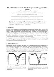
through broadband microstrip -to- coplanar strip transition. The dimensions of the proposed antenna are as follows (unit
in mm): W 1 = W 3 = W 4 = W 5 = W dri = W dir =3, W 2 = 6, W 6 = S 5 = S 6 = 1.5, L 1 = 16.5, L 2 = L 5 = 7.5, L 3 = 24, L 4 = 9, S ref =
19.5, S dir = 15, S sub = 7.5, L dri = 43.5 and L dir = 16.5.
Figure 1 Schematic drawing of Uniplanar Quasi Yagi antenna [1]
3. Simulation Results and Discussion
The analysis and design procedure is based on the full-wave electromagnetic solver based on Agilent HFSS simulator.
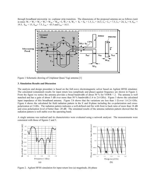
The calculated (simulated) results for input return loss (amplitude and phase) against frequency are shown in Figure 2.
From the figure we notice the antenna provides a broad bandwidth of about 50 % for VSWR < 2. The antenna is well
matched and has a gain of about 5 dB over more than 50 % bandwidth (1.6 to 2.6 GHz). Figure 3 shows the calculated
input impedance of this broadband antenna. Figure 3.b shows that the variations are less than 1 Ω over 1.6-2.6 GHz.
Figure 4 shows the calculated far field radiation pattern in the E and H-plane including the co-polarization and crosspolarization
at 2 GHz. The radiation pattern indicates a well-defined end fire with front to back ratio of more than 18 dB
and cross polarisation level of better than -20 dB. The simulated results of the antenna radiation pattern showed that the
radiation pattern is well stable over the operating band.
A single antenna was realised and its characteristics were evaluated using a network analyser. The measurements were
consistent with those of figures 2 and 3.
(a)
(b)
Figure 2. Agilent HFSS simulation for input return loss (a) magnitude, (b) phase