The Monotonicity of Information in the Central Limit Theorem and ...
The Monotonicity of Information in the Central Limit Theorem and ...
The Monotonicity of Information in the Central Limit Theorem and ...
You also want an ePaper? Increase the reach of your titles
YUMPU automatically turns print PDFs into web optimized ePapers that Google loves.
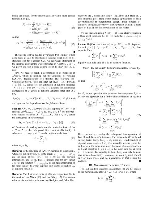
<strong>in</strong>side <strong>the</strong> <strong>in</strong>tegral for <strong>the</strong> smooth case, or via <strong>the</strong> more general<br />
formalism <strong>in</strong> [7],<br />
f ′ V (v) = ∂ ∂v E[f V 1<br />
(v − V 2 )]<br />
= E[f ′ V 1<br />
(v − V 2 )]<br />
= E[f V1 (v − V 2 )ρ V1 (v − V 2 )]<br />
so that<br />
ρ V (v) = f V ′ (v) [ ]<br />
f V (v) = E fV1 (v − V 2 )<br />
ρ V1 (v − V 2 )<br />
f V (v)<br />
= E[ρ V1 (V 1 )|V 1 + V 2 = v].<br />
(14)<br />
(15)<br />
<strong>The</strong> second tool we need is a “variance drop lemma”, which<br />
goes back at least to Hoeffd<strong>in</strong>g’s sem<strong>in</strong>al work [12] on U-<br />
statistics (see his <strong>The</strong>orem 5.2). An equivalent statement <strong>of</strong><br />
<strong>the</strong> variance drop lemma was formulated <strong>in</strong> ABBN [3]. In [4],<br />
we prove <strong>and</strong> use a more general result to study <strong>the</strong> i.n.i.d.<br />
case.<br />
First we need to recall a decomposition <strong>of</strong> functions <strong>in</strong><br />
L 2 (R n ), which is noth<strong>in</strong>g but <strong>the</strong> Analysis <strong>of</strong> Variance<br />
(ANOVA) decomposition <strong>of</strong> a statistic. <strong>The</strong> follow<strong>in</strong>g conventions<br />
are useful. [n] is <strong>the</strong> <strong>in</strong>dex set {1, 2, . . . , n}. For any<br />
s ⊂ [n], X s st<strong>and</strong>s for <strong>the</strong> collection <strong>of</strong> r<strong>and</strong>om variables<br />
{X i : i ∈ s}. For any j ∈ [n], E j ψ denotes <strong>the</strong> conditional<br />
expectation <strong>of</strong> ψ, given all r<strong>and</strong>om variables o<strong>the</strong>r than X j ,<br />
i.e.,<br />
E j ψ(x 1 , . . . , x n ) = E[ψ(X 1 , . . . , X n )|X i = x i ∀i ≠ j] (16)<br />
averages out <strong>the</strong> dependence on <strong>the</strong> j-th coord<strong>in</strong>ate.<br />
Fact II:[ANOVA DECOMPOSITION] Suppose ψ : R n → R<br />
satisfies Eψ 2 (X 1 , . . . , X n ) < ∞, i.e., ψ ∈ L 2 , for <strong>in</strong>dependent<br />
r<strong>and</strong>om variables X 1 , X 2 , . . . , X n . For s ⊂ [n], def<strong>in</strong>e<br />
<strong>the</strong> orthogonal l<strong>in</strong>ear subspaces<br />
H s = {ψ ∈ L 2 : E j ψ = ψ1 {j /∈s} ∀j ∈ [n]} (17)<br />
<strong>of</strong> functions depend<strong>in</strong>g only on <strong>the</strong> variables <strong>in</strong>dexed by<br />
s. <strong>The</strong>n L 2 is <strong>the</strong> orthogonal direct sum <strong>of</strong> this family <strong>of</strong><br />
subspaces, i.e., any ψ ∈ L 2 can be written <strong>in</strong> <strong>the</strong> form<br />
ψ = ∑<br />
ψ s , (18)<br />
where ψ s ∈ H s .<br />
s⊂[n]<br />
Remark: In <strong>the</strong> language <strong>of</strong> ANOVA familiar to statisticians,<br />
when φ is <strong>the</strong> empty set, ψ φ is <strong>the</strong> mean; ψ {1} , ψ {2} , . . . , ψ {n}<br />
are <strong>the</strong> ma<strong>in</strong> effects; {ψ s : |s| = 2} are <strong>the</strong> pairwise<br />
<strong>in</strong>teractions, <strong>and</strong> so on. Fact II implies that for any subset<br />
s ⊂ [n], <strong>the</strong> function ∑ {R:R⊂s} ψ R is <strong>the</strong> best approximation<br />
(<strong>in</strong> mean square) to ψ that depends only on <strong>the</strong> collection X s<br />
<strong>of</strong> r<strong>and</strong>om variables.<br />
Remark: <strong>The</strong> historical roots <strong>of</strong> this decomposition lie <strong>in</strong><br />
<strong>the</strong> work <strong>of</strong> von Mises [13] <strong>and</strong> Hoeffd<strong>in</strong>g [12]. For various<br />
ref<strong>in</strong>ements <strong>and</strong> <strong>in</strong>terpretations, see Kurkjian <strong>and</strong> Zelen [14],<br />
Jacobsen [15], Rub<strong>in</strong> <strong>and</strong> Vitale [16], Efron <strong>and</strong> Ste<strong>in</strong> [17],<br />
<strong>and</strong> Takemura [18]; <strong>the</strong>se works <strong>in</strong>clude applications <strong>of</strong> such<br />
decompositions to experimental design, l<strong>in</strong>ear models, U-<br />
statistics, <strong>and</strong> jackknife <strong>the</strong>ory. <strong>The</strong> Appendix conta<strong>in</strong>s a brief<br />
pro<strong>of</strong> <strong>of</strong> Fact II for <strong>the</strong> convenience <strong>of</strong> <strong>the</strong> reader.<br />
We say that a function f : R d → R is an additive function<br />
if <strong>the</strong>re exist functions f i : R → R such that f(x 1 , . . . , x d ) =<br />
∑<br />
i∈[d] f i(x i ).<br />
Lemma II:[VARIANCE DROP]Let ψ : R n−1 → R. Suppose,<br />
for each j ∈ [n], ψ j = ψ(X 1 , . . . , X j−1 , X j+1 , . . . , X n ) has<br />
mean 0. <strong>The</strong>n<br />
[<br />
∑ n ] 2<br />
E ψ j ≤ (n − 1) ∑<br />
E[ψ j ] 2 . (19)<br />
j=1<br />
j∈[n]<br />
Equality can hold only if ψ is an additive function.<br />
so that<br />
Pro<strong>of</strong>: By <strong>the</strong> Cauchy-Schwartz <strong>in</strong>equality, for any V j ,<br />
[ 1 ∑<br />
] 2<br />
V j ≤ 1 ∑<br />
[V j ] 2 , (20)<br />
n<br />
n<br />
j∈[n]<br />
[ ∑<br />
E<br />
j∈[n]<br />
j∈[n]<br />
] 2<br />
V j ≤ n ∑<br />
E[V j ] 2 . (21)<br />
j∈[n]<br />
Let Ē s be <strong>the</strong> operation that produces <strong>the</strong> component Ē s ψ =<br />
ψ s (see <strong>the</strong> appendix for a fur<strong>the</strong>r characterization <strong>of</strong> it); <strong>the</strong>n<br />
[ ∑<br />
] 2 [ ∑ ∑<br />
] 2<br />
E ψ j = E Ē s ψ j<br />
j∈[n]<br />
(a)<br />
= ∑<br />
(b)<br />
≤<br />
s⊂[n] j∈[n]<br />
s⊂[n]<br />
∑<br />
[ ∑<br />
] 2<br />
E Ē s ψ j<br />
j /∈s<br />
− 1)<br />
s⊂[n](n ∑ j /∈s<br />
(c)<br />
= (n − 1) ∑<br />
E[ψ j ] 2 .<br />
j∈[n]<br />
E [ Ē s ψ j<br />
] 2<br />
(22)<br />
Here, (a) <strong>and</strong> (c) employ <strong>the</strong> orthogonal decomposition <strong>of</strong><br />
Fact II <strong>and</strong> Parseval’s <strong>the</strong>orem. <strong>The</strong> <strong>in</strong>equality (b) is based<br />
on two facts: firstly, E j ψ j = ψ j s<strong>in</strong>ce ψ j is <strong>in</strong>dependent <strong>of</strong><br />
X j , <strong>and</strong> hence Ēsψ j = 0 if j ∈ s; secondly, we can ignore <strong>the</strong><br />
null set φ <strong>in</strong> <strong>the</strong> outer sum s<strong>in</strong>ce <strong>the</strong> mean <strong>of</strong> a score function<br />
is 0, <strong>and</strong> <strong>the</strong>refore {j : j /∈ s} <strong>in</strong> <strong>the</strong> <strong>in</strong>ner sum has at most<br />
n − 1 elements. For equality to hold, Ē s ψ j can only be nonzero<br />
when s has exactly 1 element, i.e., each ψ j must consist<br />
only <strong>of</strong> ma<strong>in</strong> effects <strong>and</strong> no <strong>in</strong>teractions, so that it must be<br />
additive.<br />
III. MONOTONICITY IN THE IID CASE<br />
For i.i.d. r<strong>and</strong>om variables, <strong>in</strong>equalities (2) <strong>and</strong> (3) reduce<br />
to <strong>the</strong> monotonicity H(Y n ) ≥ H(Y m ) for n > m, where<br />
Y n = 1 √ n<br />
n ∑<br />
i=1<br />
X i . (23)


