The Monotonicity of Information in the Central Limit Theorem and ...
The Monotonicity of Information in the Central Limit Theorem and ...
The Monotonicity of Information in the Central Limit Theorem and ...
Create successful ePaper yourself
Turn your PDF publications into a flip-book with our unique Google optimized e-Paper software.
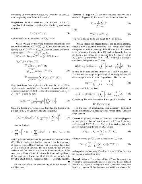
For clarity <strong>of</strong> presentation <strong>of</strong> ideas, we focus first on <strong>the</strong> i.i.d.<br />
case, beg<strong>in</strong>n<strong>in</strong>g with Fisher <strong>in</strong>formation.<br />
Proposition I:[MONOTONICITY OF FISHER INFORMA-<br />
TION]For i.i.d. r<strong>and</strong>om variables with absolutely cont<strong>in</strong>uous<br />
densities,<br />
I(Y n ) ≤ I(Y n−1 ), (24)<br />
with equality iff X 1 is normal or I(Y n ) = ∞.<br />
Pro<strong>of</strong>: We use <strong>the</strong> follow<strong>in</strong>g notational conventions: <strong>The</strong><br />
(unnormalized) sum is V n = ∑ i∈[n] X i, <strong>the</strong> leave-one-out sum<br />
leav<strong>in</strong>g out X j is V (j) = ∑ i≠j X i, <strong>and</strong> <strong>the</strong> normalized leaveone-out<br />
sum is Y (j) = √ 1<br />
n−1<br />
∑i≠j X i.<br />
If X ′ = aX, <strong>the</strong>n ρ X ′(X ′ ) = 1 a ρ X(X); hence<br />
ρ Yn (Y n ) = √ nρ Vn (V n )<br />
(a)<br />
= √ nE[ρ V (j)(V (j) )|V n ]<br />
√ n<br />
=<br />
n − 1 E[ρ Y (j)(Y (j) )|V n ]<br />
(b)<br />
=<br />
1<br />
√<br />
n(n − 1)<br />
n<br />
∑<br />
j=1<br />
E[ρ Y (j)(Y (j) )|Y n ].<br />
(25)<br />
Here, (a) follows from application <strong>of</strong> Lemma I to V n = V (j) +<br />
X j , keep<strong>in</strong>g <strong>in</strong> m<strong>in</strong>d that Y n−1 (hence V (j) ) has an absolutely<br />
cont<strong>in</strong>uous density, while (b) follows from symmetry. Set ρ j =<br />
ρ Y (j)(Y (j) ); <strong>the</strong>n we have<br />
ρ Yn (Y n ) =<br />
[<br />
1 ∑ n ∣ ∣∣∣<br />
√ E ρ j Y n<br />
]. (26)<br />
n(n − 1)<br />
j=1<br />
S<strong>in</strong>ce <strong>the</strong> length <strong>of</strong> a vector is not less than <strong>the</strong> length <strong>of</strong> its<br />
projection (i.e., by Cauchy-Schwartz <strong>in</strong>equality),<br />
[ n<br />
I(Y n ) = E[ρ Yn (Y n )] 2 1<br />
≤<br />
n(n − 1) E ∑<br />
] 2<br />
ρ j . (27)<br />
Lemma II yields<br />
[<br />
∑ n ] 2<br />
E ρ j ≤ (n − 1) ∑<br />
j=1<br />
j∈[n]<br />
j=1<br />
E[ρ j ] 2 = (n − 1)nI(Y n−1 ), (28)<br />
which gives <strong>the</strong> <strong>in</strong>equality <strong>of</strong> Proposition I on substitution <strong>in</strong>to<br />
(27). <strong>The</strong> <strong>in</strong>equality implied by Lemma II can be tight only<br />
if each ρ j is an additive function, but we already know that<br />
ρ j is a function <strong>of</strong> <strong>the</strong> sum. <strong>The</strong> only functions that are both<br />
additive <strong>and</strong> functions <strong>of</strong> <strong>the</strong> sum are l<strong>in</strong>ear functions <strong>of</strong> <strong>the</strong><br />
sum; hence <strong>the</strong> two sides <strong>of</strong> (24) can be f<strong>in</strong>ite <strong>and</strong> equal only<br />
if <strong>the</strong> score ρ j is l<strong>in</strong>ear, i.e., if all <strong>the</strong> X i are normal. It is<br />
trivial to check that X 1 normal or I(Y n ) = ∞ imply equality.<br />
We can now prove <strong>the</strong> monotonicity result for entropy <strong>in</strong><br />
<strong>the</strong> i.i.d. case.<br />
<strong>The</strong>orem I: Suppose X i are i.i.d. r<strong>and</strong>om variables with<br />
densities. Suppose X 1 has mean 0 <strong>and</strong> f<strong>in</strong>ite variance, <strong>and</strong><br />
<strong>The</strong>n<br />
Y n = 1 √ n<br />
n ∑<br />
i=1<br />
X i (29)<br />
H(Y n ) ≥ H(Y n−1 ). (30)<br />
<strong>The</strong> two sides are f<strong>in</strong>ite <strong>and</strong> equal iff X 1 is normal.<br />
Pro<strong>of</strong>: Recall <strong>the</strong> <strong>in</strong>tegral form <strong>of</strong> <strong>the</strong> de Bruijn identity,<br />
which is now a st<strong>and</strong>ard method to “lift” results from Fisher<br />
divergence to relative entropy. This identity was first stated<br />
<strong>in</strong> its differential form by Stam [2] (<strong>and</strong> attributed by him to<br />
de Bruijn), <strong>and</strong> proved <strong>in</strong> its <strong>in</strong>tegral form by Barron [6]: if<br />
X t is equal <strong>in</strong> distribution to X + √ tZ, where Z is normally<br />
distributed <strong>in</strong>dependent <strong>of</strong> X, <strong>the</strong>n<br />
H(X) = 1 2 log(2πev) − 1 2<br />
∫ ∞<br />
0<br />
[<br />
I(X t ) − 1<br />
v + t<br />
]<br />
dt (31)<br />
is valid <strong>in</strong> <strong>the</strong> case that <strong>the</strong> variances <strong>of</strong> Z <strong>and</strong> X are both v.<br />
This has <strong>the</strong> advantage <strong>of</strong> positivity <strong>of</strong> <strong>the</strong> <strong>in</strong>tegr<strong>and</strong> but <strong>the</strong><br />
disadvantage that is seems to depend on v. One can use<br />
∫ ∞<br />
[ 1<br />
log v =<br />
1 + t − 1 ]<br />
(32)<br />
v + t<br />
to re-express it <strong>in</strong> <strong>the</strong> form<br />
H(X) = 1 2 log(2πe) − 1 2<br />
0<br />
∫ ∞<br />
0<br />
[<br />
I(X t ) − 1 ]<br />
dt. (33)<br />
1 + t<br />
Comb<strong>in</strong><strong>in</strong>g this with Proposition I, <strong>the</strong> pro<strong>of</strong> is f<strong>in</strong>ished.<br />
IV. EXTENSIONS<br />
For <strong>the</strong> case <strong>of</strong> <strong>in</strong>dependent, non-identically distributed<br />
(i.n.i.d.) summ<strong>and</strong>s, we need a general version <strong>of</strong> <strong>the</strong> “variance<br />
drop” lemma.<br />
Lemma III:[VARIANCE DROP: GENERAL VERSION]Suppose<br />
we are given a class <strong>of</strong> functions ψ (s) : R |s| → R for any<br />
s ∈ Ω m , <strong>and</strong> Eψ (s) (X 1 , . . . , X m ) = 0 for each s. Let w be<br />
any probability distribution on Ω m . Def<strong>in</strong>e<br />
U(X 1 , . . . , X n ) = ∑<br />
s∈Ω m<br />
w s ψ (s) (X s ), (34)<br />
where we write ψ (s) (X s ) for a function <strong>of</strong> X s .<strong>The</strong>n<br />
( ) n − 1 ∑<br />
EU 2 ≤<br />
w<br />
m − 1<br />
sE[ψ 2 (s) (X s )] 2 , (35)<br />
s∈Ω m<br />
<strong>and</strong> equality can hold only if each ψ (s) is an additive function<br />
(<strong>in</strong> <strong>the</strong> sense def<strong>in</strong>ed earlier).<br />
Remark: When ψ (s) = ψ (i.e., all <strong>the</strong> ψ (s) are <strong>the</strong> same), ψ is<br />
symmetric <strong>in</strong> its arguments, <strong>and</strong> w is uniform, <strong>the</strong>n U def<strong>in</strong>ed<br />
above is a U-statistic <strong>of</strong> degree m with symmetric, mean zero<br />
kernel ψ. Lemma III <strong>the</strong>n becomes <strong>the</strong> well-known bound for


