Excited state properties p p - WIEN 2k
Excited state properties p p - WIEN 2k
Excited state properties p p - WIEN 2k

You also want an ePaper? Increase the reach of your titles
YUMPU automatically turns print PDFs into web optimized ePapers that Google loves.
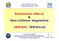
<strong>Excited</strong> <strong>state</strong> <strong>properties</strong><br />
p<br />
within <strong>WIEN</strong><strong>2k</strong><br />
Claudia Ambrosch-Draxl, University of Leoben, Austria<br />
Chair of Atomistic Modelling and Design of Materials
Beyond the ground <strong>state</strong><br />
Basics about light scattering<br />
The dielectric i tensor<br />
The <strong>WIEN</strong><strong>2k</strong> code<br />
Outlook<br />
The program<br />
Input / output<br />
Examples<br />
TDDFT versus manybody perturbation theory<br />
Contents
Light-Matter Interaction
Resonse to external electric field E<br />
Polarizability<br />
Linear approximation<br />
susceptibility χ<br />
conductivity σ<br />
dielectric tensor<br />
∋<br />
Fourier transform<br />
Light-Matter Interaction
The dielectric tensor<br />
Free electrons: the Lindhard formula<br />
Bloch electrons<br />
intraband<br />
interband<br />
Light-Matter Interaction
Interband contributions<br />
Independent particle approximation<br />
RPA<br />
En<br />
nergy<br />
c k<br />
hω<br />
E F<br />
hω<br />
S<br />
E<br />
v k<br />
Light-Matter Interaction
Optical constants<br />
Complex dielectric tensor<br />
Optical conductivity<br />
Complex refractive index<br />
Reflectivity<br />
Absorption coefficient<br />
Loss function<br />
Light-Matter Interaction
Intraband contributions<br />
Dielectric tensor<br />
Ene<br />
ergy<br />
E F<br />
Optical conductivity<br />
Drude-like terms<br />
plasma frequency<br />
Light-Matter Interaction
Sumrules<br />
Light-Matter Interaction
Symmetry<br />
triclinic<br />
monoclinic (α,β=90°)<br />
orthorhombic<br />
tetragonal, hexagonal<br />
cubic<br />
Light-Matter Interaction
Magneto-optics: optics: example<br />
without magnetic field, spin-orbit coupling: cubic<br />
KK<br />
with magnetic field ║z, spin-orbit coupling: tetragonal<br />
KK<br />
KK<br />
Light-Matter Interaction
The Program …
SCF cycle → converged potential<br />
x kgen<br />
→ dense mesh<br />
x lapw1 → Kohn-Sham <strong>state</strong>s (higher E max )<br />
x lapw2 -Fermi → Fermi distribution<br />
optic package<br />
x optic<br />
x joint<br />
x kram<br />
→ momentum matrix elements<br />
→ tensor components<br />
→ optical constants<br />
↔ life time broadening<br />
↔ scissors shift<br />
The Program Flow
optic<br />
Al.inop<br />
2000 1 number of k-points, first k-point<br />
-5.0 2.2 energy window for matrix elements<br />
1 number of cases (see choices)<br />
1 Re <br />
OFF write unsymmetrized matrix elements to file?<br />
Ni.inop<br />
800 1 number of k-points, first k-point<br />
-5.0 50 50 5.0 energy window for matrix elements<br />
3 number of cases (see choices)<br />
1 Re <br />
3 Re<br />
<br />
7 Im <br />
OFF<br />
Choices:<br />
1......Re <br />
2......Re <br />
3......Re <br />
4......Re <br />
5......Re <br />
6......Re <br />
7......Im <br />
8......Im <br />
9......Im <br />
Inputs
joint<br />
Al.injoint<br />
1 18 lower and upper band index<br />
0.000 0.001 1.000 E min , dE, Emax [Ry]<br />
eV<br />
output units eV / Ry<br />
4 switch<br />
1 number of columns to be considered<br />
0.1 0.2 broadening for Drude term(s)<br />
choose gamma for each case!<br />
0...JOINT DOS for each band combination<br />
1...JOINT DOS<br />
sum over all band combinations<br />
2...DOS for each band<br />
3...DOS sum over all bands<br />
4...Im(EPSILON) total<br />
5...Im(EPSILON) for each band combination<br />
6...intraband contributions<br />
7...intraband contributions including band analysis<br />
Inputs
kram<br />
Al.inkram<br />
0.1 broadening gamma<br />
0.0 energy shift (scissors operator)<br />
1 add intraband contributions 1/0<br />
12.6 plasma frequency<br />
0.2 Γ(s) for intraband part<br />
Si.inkram<br />
0.05 broadening gamma<br />
1.00 energy shift (scissors operator)<br />
0<br />
....<br />
80<br />
70 Silicon<br />
60<br />
Imε<br />
50<br />
40<br />
Reε<br />
30<br />
20<br />
10<br />
0<br />
-10<br />
Γ=0.05eV<br />
-20<br />
0 1 2 3 4 5 6<br />
Energy [eV]<br />
Inputs
optic<br />
joint<br />
kram<br />
case.symmat<br />
case.mommat<br />
case.joint<br />
case.epsilon<br />
case.sigmaksigmak<br />
case.refraction<br />
case.absorpabsorp<br />
case.eloss<br />
Outputs
Results …
Convergence<br />
m ε<br />
nterba and Im<br />
I<br />
175<br />
150<br />
125<br />
100<br />
75<br />
50<br />
25<br />
165k<br />
286k<br />
560k<br />
1240k<br />
2456k<br />
3645k<br />
4735k<br />
12.8<br />
12.7 12.6<br />
ω p<br />
12.5<br />
12.4<br />
12.3<br />
12.2<br />
12.1<br />
12.0<br />
0 1000 2000 3000 4000 5000<br />
k-points in IBZ<br />
0<br />
0.0 0.5 1.0 1.5 2.0 2.5 3.0 3.5 4.0<br />
Energy [eV]<br />
Example: Al
Sumrules<br />
N eff<br />
[ele ectrons s]<br />
5<br />
4<br />
3<br />
2<br />
1<br />
165 k-points<br />
4735 k-points<br />
Experiment<br />
0<br />
0 10 20 30 40 50 60 70 80 90 100<br />
Energy [eV]<br />
Example: Al
Loss function<br />
120<br />
100<br />
Loss fu unctio n<br />
80<br />
intraband<br />
60<br />
40 total<br />
20 interband<br />
0<br />
0 5 10 15 20<br />
Energy [eV]<br />
Example: Al
Band structure<br />
Band structure<br />
16<br />
18<br />
non-relativistic<br />
scalar-relativistic<br />
relativistic<br />
8<br />
10<br />
12<br />
14<br />
16<br />
s<br />
2<br />
4<br />
6<br />
8<br />
rgy [eV]<br />
s<br />
d<br />
f<br />
pd<br />
pf<br />
p<br />
-6<br />
-4<br />
-2<br />
0<br />
Energy<br />
pd<br />
-12<br />
-10<br />
-8<br />
-6<br />
K<br />
X<br />
G<br />
L<br />
W<br />
W<br />
K<br />
X<br />
G<br />
L<br />
W<br />
W<br />
K<br />
X<br />
G<br />
L<br />
W<br />
W<br />
Example: Au
Density of <strong>state</strong>s<br />
4<br />
DOS<br />
[ <strong>state</strong>s per<br />
eV and cell]<br />
3 total<br />
2<br />
1<br />
0<br />
3 d<br />
2<br />
1<br />
0<br />
0.4<br />
0.2<br />
s<br />
0.0<br />
0.4 p<br />
0.2<br />
0.0<br />
0.4<br />
0.2<br />
f<br />
0.0<br />
-10 0 10 20 30 40<br />
Energy [eV]<br />
S / energy 2<br />
joint DOS<br />
0.14<br />
0.12<br />
0.10<br />
0.08<br />
0.06<br />
0.04<br />
0.02<br />
0.00<br />
non-relativistic<br />
scalar-relativistic<br />
relativistic<br />
0 5 10 15 20 25<br />
Energy [eV]<br />
Example: Au
Dielectric tensor<br />
joint DOS / ener ergy 2<br />
0.14<br />
0.12<br />
0.10<br />
0.08<br />
0.06<br />
0.04<br />
0.02<br />
non-relativistic<br />
scalar-relativistic<br />
relativistic<br />
0.00<br />
0 5 10 15 20 25<br />
Energy [eV]<br />
Diele lectric Functio ction<br />
14<br />
12<br />
10<br />
8<br />
6<br />
4<br />
2<br />
0<br />
-2<br />
Au<br />
12 Ree<br />
non-relativistic<br />
scalar-relativistic<br />
10<br />
8<br />
Ime<br />
6<br />
4<br />
2<br />
0<br />
-2<br />
12<br />
10<br />
relativistic<br />
8<br />
6<br />
4<br />
2<br />
0<br />
-2<br />
0 5 10 15 20 25 30 35<br />
Energy [eV]<br />
Example: Au
Theory versus experiment<br />
K. Glantschnig and C. Ambrosch-Draxl (preprint)<br />
Example: Pt
Whom to ask?<br />
Robert Abt<br />
C. Ambrosch-Draxl and J. O. Sofo<br />
Linear optical <strong>properties</strong> of solids within the full-potential linearized<br />
augmented planewave method<br />
Comp. Phys. Commun. 175, , 1-1414 (2006)<br />
People
… and Beyond
Discrepancies<br />
Ground <strong>state</strong><br />
xc functionals<br />
<strong>Excited</strong> <strong>state</strong><br />
Interpretation in terms of ground <strong>state</strong> <strong>properties</strong><br />
Interpretation within one-particle picture<br />
Response function<br />
Manybody treatment needed<br />
2 routes<br />
Time-dependent d DFT (TDDFT)<br />
Manybody perturbation theroy (MBPT)<br />
Beyond the Ground State
MBPT<br />
mixing of concepts<br />
4 point functions involved<br />
very demanding<br />
2 steps: GW & BSE<br />
linear-response regime<br />
TDDFT<br />
keeps spirit of DFT<br />
2 point functions<br />
less demanding<br />
1 functional needed<br />
in principle one step<br />
in practice: GW needed<br />
generally applicable<br />
linear-response regime<br />
strong laser fields etc.<br />
G. Onida, L. Reining, and A. Rubio, Rev. Mod. Phys. 74, 601 (2002)<br />
Beyond the Ground State