corresponding pdf

SAT scores — knitr
STT 3820
Alan T. Arnholt
March 18, 2012
1 SAT scores
How strong was the association between student scores on the Math and Verbal sections of the old SAT?
Scores on each ranged from 200 to 800 and were widely used by college admission offices.
a) Is there evidence of an association between Math and Verbal scores? Write an appropriate hypothesis.
b) Discuss the assumptions for inference.
c) Test your hypothesis and state an appropriate conclusion.
d) Find a 90% confidence interval for the slope of the true line describing the association between Math and
Verbal scores.
e) Explain, in this context, what your confidence interval means.
f) Find a 90% confidence interval for the mean SAT-Math score for all students with an SAT-Verbal score of
500.
g) Find a 90% prediction interval for the Math score of the senior class president if you know that she scored
710 on the Verbal section.
2 Answers
(a) The hypotheses to test for a linear relationship between SAT Verbal and SAT Math scores are: H 0 : β 1 = 0
versus H A : β 1 ≠ 0.
(b) Checking Assumptions
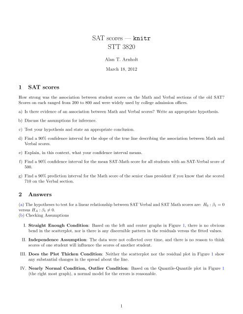
I. Straight Enough Condition: Based on the left and center graphs in Figure 1, there is no obvious
bend in the scatterplot, nor is there is any discernible pattern in the residuals versus the fitted values.
II. Independence Assumption: The data were not collected over time, and there is no reason to think
scores of one student will influence the scores of another student.
III. Does the Plot Thicken Condition: Neither the scatterplot nor the residual plot in Figure 1 show
any substantial changes in the spread about the line.
IV. Nearly Normal Condition, Outlier Condition: Based on the Quantile-Quantile plot in Figure 1
(the right most graph), a normal model for the errors is reasonable.
1

(c) The t-value for testing H 0 : β 1 = 0 versus H A : β 1 ≠ 0 is 11.8802, which has a corresponding p-value of
9.7478 × 10 −24 suggesting there is strong evidence of a positive linear relationship between Sat Verbal and
Sat Math scores.
(d) The 90% confidence interval for the slope of the true line is (0.5811, 0.7691).
(e) Based on the sample, we are 90% confident that average SAT Math scores increase between 0.5811 and
0.7691 points for each additional point scored on the SAT Verbal test.
(f) We are 90% confident that the mean Math score for students with a Verbal score of 500 is between 534
and 560.
(g) We are 90% confident that the Math score for the senior class president with a Verbal score of 710 will be
between 569 and 808. Since the highest score one can recieve on the test in any one portion is an 800, we are
90% confident the senior class president will have math score between 569 and 800.
3 Mechanics
> site SAT str(SAT)
’data.frame’: 162 obs. of 2 variables:
$ Math : int 450 540 570 400 590 610 610 570 720 640 ...
$ Verbal: int 450 640 590 400 600 610 630 660 660 590 ...
> modPROB18 summary(modPROB18)
Call:
lm(formula = Math ~ Verbal, data = SAT)
Residuals:
Min 1Q Median 3Q Max
-173.59 -47.60 1.16 45.09 259.66
Coefficients:
Estimate Std. Error t value Pr(>|t|)
(Intercept) 209.5542 34.3494 6.1 7.7e-09 ***
Verbal 0.6751 0.0568 11.9 < 2e-16 ***
---
Signif. codes: 0 ’***’ 0.001 ’**’ 0.01 ’*’ 0.05 ’.’ 0.1 ’ ’ 1
Residual standard error: 71.8 on 160 degrees of freedom
Multiple R-squared: 0.469,Adjusted R-squared: 0.465
F-statistic: 141 on 1 and 160 DF, p-value:
+ MODprob18 ggplot(data = SAT, aes(x = Verbal, y = Math)) + geom_point() +
+ geom_smooth(method = "lm")
2

ggplot(data = MODprob18, aes(x = .fitted, y = .resid)) +
+ geom_point() + geom_smooth() + geom_abline(intercept = 0, slope = 0,
+ color = "red") + scale_y_continuous(name = "Residuals") + scale_x_continuous(name =
"Fitted Values")
> ggplot(data = MODprob18, aes(sample = .resid)) + stat_qq()
800
●
●
●
●
●
●
Math
700
600
500
400
●
● ● ● ●
●
● ● ● ●●
●
● ● ● ●
● ●
●
● ●
●●
●
●
● ●
● ●●●
● ● ●
●
●
●●
●
●
●
● ●
● ●
●
●
● ● ●
●
● ● ●
●
●
●●
● ● ●
● ● ● ●
●●
●
● ● ●●
●
● ●●
● ● ● ●
●
●
●
● ●
●
● ● ● ● ● ● ● ●
● ● ● ● ●
● ●
●
● ● ●●
● ●
●●
●●
●
● ●
●
● ●
●
●
●
●
●
●
●
●
● ●
●
●
●
● ●
●
● ● ●
●●
●
●
●
Residuals
200
100
0
−100
●
●
●
●
●
●
●
● ● ●
●
●
●
● ●
●
●
●
●
●
●
●●
● ●
● ●
● ● ●
●
● ●
● ●
● ●
●
● ●
●
●
● ● ● ●
●
●
●
●
●
●●
●
●
●
● ●
●● ● ● ●
●●
●
● ●
●
●
●
●●
●
● ●●
●
●
● ●
●
● ● ●
●
● ● ●●
● ●
●
● ● ● ●
●
●
●
●●
●
●
●
●
●
● ●
● ● ●
●
●
●
●
● ●
●
●
●
● ●●
●
●
● ●
●
●
●
●
●
● ●
● ●
●
●
●
●
●
●
●
●
sample
200
100
0
−100
●
● ●●●●● ● ●●●●●●●●●●● ●●●● ●
● ●● ●
● ●●●●●●●●●●●●●●●●●● ●
400 500 600 700 800
Verbal
450 500 550 600 650 700
Fitted Values
−2 −1 0 1 2
theoretical
Figure 1: Left graph shows scatterplot of Math versus Verbal scores with superimposed least squares line,
middle graph shows the Residuals versus Fitted Values, the right graph shows a normal quantile-quantile plot
of of the residuals
> confint(modPROB18, level = 0.9)
5 % 95 %
(Intercept) 152.7255 266.3829
Verbal 0.5811 0.7691
> confint(modPROB18, "Verbal", level = 0.9)
5 % 95 %
Verbal 0.5811 0.7691
> CI PI CI[2:3]
[1] 534.1 560.1
> PI[2:3]
[1] 569.3 808.4
3