Encode Decode

CODE.PPT 6.1
CODE.PPT 6.2
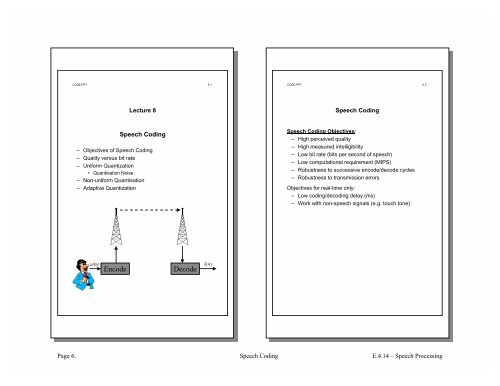
Lecture 8
Speech Coding
Speech Coding
– Objectives of Speech Coding
– Quality versus bit rate
– Uniform Quantization
• Quantisation Noise
– Non-uniform Quantisation
– Adaptive Quantization
Speech Coding Objectives:
– High perceived quality
– High measured intelligibility
– Low bit rate (bits per second of speech)
– Low computational requirement (MIPS)
– Robustness to successive encode/decode cycles
– Robustness to transmission errors
Objectives for real-time only:
– Low coding/decoding delay (ms)
– Work with non-speech signals (e.g. touch tone)
s(n)
Encode
Decode
sˆ ( n)
Page 6. Speech Coding E.4.14 – Speech Processing

CODE.PPT 6.3
CODE.PPT 6.4
Objective Assessment
Subjective Assessment
– MOS (Mean Opinion Score): a panel of test listeners
rates the quality 1 to 5.
1=bad, 2=poor, 3=fair, 4=good, 5=excellent.
– DRT (Diagnostic Rhyme Test): listeners choose
between pairs of rhyming words (e.g. veal/feel)
– DAM (Diagnostic Acceptability Measure): Trained
listeners judge various factors e.g. muffledness,
buzziness, intelligibility
Quality versus data rate (8kHz sample rate)
Not terribly closely related to subjective quality.
– Segmental SNR: average value of 10log 10 (E speech /E error )
evaluated in 20 ms frames.
No good for coding schemes that can introduce delays as a
one-sample time shift causes a huge decrease in SNR.
– Spectral distances
Based on the power spectrum of the original and codeddecoded
speech signals, P(ω) and Q(ω). denotes the
average over the frequency range 0 … 2π.
Itakura Distance
⎛
log⎜
⎝
P(
ω)
⎞
⎟
−
Q(
ω)
⎠
⎛ P(
ω)
⎞
log⎜
⎟
⎝ Q(
ω)
⎠
music:
5 (excellent)
Mean Opinion Score
4 (good)
3 (fair)
2 (poor)
MELP
1996
LPC10
1984
CELP
1996
GSM2
1994
CELP
1991
LD-CELP
1994
GSM
1987
ADPCM
1984
A/µ law
1972
PCM16
2k 4k 8k 16k 32k 64k 128k
Bits per second
Itakura-Saito Distance
P(
ω)
⎛ P(
ω)
⎞
− log⎜
⎟ −1
Q(
ω)
⎝ Q(
ω)
⎠
Both distances are evaluated over 20 ms frames and
averaged.
If you do LPC analysis on the original and coded speech,
both these distances may also be calculated directly from
the LPC coefficients.
Neither is a true distance metric since they are
asymmetrical:
d P, Q ≠ d Q,
P
( ) ( )
Page 6. Speech Coding E.4.14 – Speech Processing

CODE.PPT 6.5
CODE.PPT 6.6
Quantization Errors
Linear PCM – Pulse Code Modulation
Input &
Output
Signals
Quantisation
Error
Coding/Decoding introduces a quantisation error of ±½w
If input values are uniformly distributed within the bin, the
mean square quantisation error is:
+ ½w
2
x
dx x w
∫ = ⎡ 0289w
w ⎣ ⎢ ⎤
⎥ = ⇒ rms error = .
3w⎦
12
−½w
3
+ ½w
2
−½w
If the quantisation levels are uniformly spaced, w is the
separation between adjacent output values and is called a
Least Significant Bit (LSB)
RMS Quantization Noise is 0.289w = 0.289 LSB
Sine Wave SNR
Full scale sine wave has peak of 0.5 w × 2 n and an rms
value of 0.354 w × 2 n
SNR = 20log
10
⎛rms of maximal sine wave⎞
⎜
⎟
⎝ rms of quantisation noise ⎠
⎛ 0354 . n⎞
= 20log10⎜
× 2 ⎟ = 20log 10( 122 . ) + 20nlog 10( 2)
⎝ 0289 . ⎠
= 176 . + 602 . n dB
Speech SNR
2 n w = 2 n LSB
RMS value of speech or music signal is 10 to 20 dB less
than a sine wave with the same peak amplitude. SNR is 10
to 20 dB worse.
Page 6. Speech Coding E.4.14 – Speech Processing

CODE.PPT 6.7
CODE.PPT 6.8
Non-Uniform Quantization
Non-uniform PCM @ 64 kb/s (f s = 8kHz)
Speech pdf
Uniform
A-law
µ-law
– RMS quantization error = 0.29 ×Quantization step
– Low level signals are commoner than high level ones
– Conclusion:
Make quantization steps closer together at the
commoner signal levels.
Instead of linear coding, use floating point with smaller
intervals for more frequently occuring signal levels:
s = sign bit (1 = +ve)
e = 3-bit exponent
m = 4-bit mantissa Range of values ≈ ±4095
0dB ≈ 2002(µ) or 2017(A) rms
µ-law (US standard):
Bin centres at ±{(m+16½) 2 e – 16½}
Bin widths: 2 e
A-law (European standard):
Bin centres at ±(m+16½) 2 e for e>0 and ±(2m+1) for e=0
Bin widths: 2 e for e>0 and 2 for e=0
For transmission, A-law is XORed with $55 and µ-law with $7F
Performance: MOS=4.3, DRT=95, DAM=73, SNR ≤38dB
For sine waves > –30dB, SNR is almost constant at 38dB
At very low signal levels (–40dB) µ-law≈13 bit, A-law ≈12 bit linear
Page 6. Speech Coding E.4.14 – Speech Processing

CODE.PPT 6.9
CODE.PPT 6.10
Quantising a Gaussian Signal
Adaptive Quantization
a 1 a 2
x 1 x 2 … … x n–1
Input values from a i–1 to a i are converted to x i .
For minimum error we must have a i = ½(x i + x i+1 )
x n
For this range of x, the quantisation error is q(x) = x i – x
The mean square quantisation error is
+∞
∫
n
a
2 2
∑ ∫ ( i )
ai−1
i = 1
i
E = p( x) q ( x) dx = p( x)
x − x dx
−∞
Differentiating w.r.t. x i : ∂E
ai
= px( x x)
dx
∂x
∫ −2
( ) −
a
i
i−1
i
ai
ai
= 2x p( x) dx−2
xp( x)
dx
Find minimum error by setting the derivative to zero
x
i
=
∫
∫
ai
ai−1
ai
ai−1
xp( x)
dx
pxdx ( )
To find optimal {x i }, take an initial guess and iteratively use
the above equation to improve their estimates.
For 15 bins, SNR = 19.7dB
i
∫
∫
ai−1 ai−1
⇔ x i is at the centroid of its bin.
– We want to use smaller steps when the signal level is
small
– We can adjust the step sizes automatically according
to the signal level:
• If almost all samples correspond to the central few
quantisation levels, we must reduce the step size
• If many samples correspond to high quantisation levels,
we must increase the step sizes
Page 6. Speech Coding E.4.14 – Speech Processing

CODE.PPT 6.11
CODE.PPT 6.12
Adaptive Quantization
Scale Factor Updates
5
– Transmitter:
• Divide input signal by k
• Q quantises to 15 levels
• Transmit one of 15 code words
• Update k to new value
– Receiver:
• Inverse quantiser, Q –1 converts received code word to a
number
• Multiply by k to give output value
• Update k to new value
– Update Algorithm
• Decrease k whenever a small code word is
transmitted/received
• Increase k whenever a large code word is
transmitted/received
• Transmitter and Receiver will always have the same
value of k
multiplication factor, M
4.5
4
3.5
3
2.5
2
1.5
1
0.5
-8 -6 -4 -2 0 2
Code word
– k is decreased slightly for “zero” code word (× 0.98)
– k is increased rapidly for extreme code words (× 4.6)
– k is increased slightly for other code words
– Calculation done in log domain:
log( kn) = 097 . log( kn−1)
+ log( M)
“leakage factor” of 0.97 allows recovery from
transmission errors.
Page 6. Speech Coding E.4.14 – Speech Processing

CODE.PPT 6.13
CODE.PPT 6.14
Adaptive Quantization
Lecture 9
Original
Quantised (15 levels)
Adaptive Differential PCM
– Differential Speech Coding
– ADPCM coding
• Prediction Filter
• Filter Adaptation
• Stability Triangle
Error
k
Small signal sections ⇒ small k ⇒ small errors
Page 6. Speech Coding E.4.14 – Speech Processing

CODE.PPT 6.15
CODE.PPT 6.16
Differential PCM (DPCM)
a i
(n)
x(n)
x(n)
+ + Predictor
s(n) +
+ – e(n)
d(n)
Quantiser
+
a^
i
(n)
q(n)
x(n) ^
+ + Predictor
d(n) ^ +
– The encoder contains a complete copy of the decoder
– If no transmission errors, yn !( ) ≡ yn ( ) etc
– Quantisation noise, q(n) = d(n) – e(n)
– Output y(n) = x(n) + d(n) = s(n) – e(n) + d(n) = s(n) + q(n)
Es
Es
Ee
E
SNR = = × = Gp
×
E E E E
q
e
– The predictor is chosen to maximize the prediction
gain: G p = signal energy ÷ prediction error energy.
– E e /E q is the quantiser SNR
– Thea i can be one of:
• fixed constants
• transmitted seperately
• deduced from d(n) and/or y(n)
q
e
q
y(n)
y(n) ^
Adaptive Differential PCM (ADPCM) @ 32 kbit/s
kn ( )
xn ()
b i a i
Scale Factor B + A
–
sn ( ) en ( )
+ Q Q –1 dn ()
÷ × + +
b
^ i a^
i
Q –1
Scale Factor
^kn
( )
+ +
– Quantiser has 15 levels ⇒ 4 bits × 8kHz = 32 kbit/s
– Code 0000 is never transmitted which makes
transmission easier
– Quantisation levels assume e(n) ÷ k(n) is Gaussian
with unit variance. Scale factor k(n) is adjusted to
make this true
– The LPC filter, A, is only of order 2 so that it is easy to
ensure stability.
– The FIR filter, B, is of order 6 and partially makes up
for the short A.
Performance: MOS=4.1, DRT=94, DAM=68, 2 MIPS
×
B
dn ^( )
A
yn ( )
yn ^( )
Page 6. Speech Coding E.4.14 – Speech Processing

CODE.PPT 6.17
CODE.PPT 6.18
Filter Adaptation
Prediction Filter
We adjust the b i to reduce the signal d 2 (n) by moving them
∂
∂
a little in the direction − ( ) =−
∂b d 2
n d n dn ( )
( ) 2 ( )
i
∂bi
Filters:
−1
−2
Az () = az 1 + az 2
We express D in terms of previous values of D:
−1
−2
−3
−4
−5
−6
Bz () = bz 1 + bz 2 + bz 3 + bz 4 + bz 5 + bz 6
Note that ∂ D S Q X S Q A +
= + − = + −
B A ∂B
i
= = z
− 1−
A D
∂ai
∂b
∂D
i
−i
1
z
Note that A(z) and B(z) filters involve only past values
b A D z −i
D ∂dn
( )
=− ≈− ⇒ ≈−dn
( −i)
∂ i 1−
∂bi
Signals:
1 B
Y = D + BD + AY ⇒ Y = + 1−
A D
X BD AY Y D A +
= + = − =
B 1−
A D
D= S+ Q− X = S+ Q− Y+ D ⇒ Y = S+
Q
In the absence of transmission errors, the y(n) output at the
receiver and transmitter will be identical and equal to the
input speech plus the quantisation noise
Hence we want to adjust b i in the direction d(n)d(n-i):
The function sgn() takes the sign of its argument. The
0.996 leakage factor assists in recovery from transmission
errors and prevents b i from exceeding ±2.
( )
b ← 0. 996b + 0. 008× sgn d( n) d( n−i)
i
i
Adjustment of a i is similar but more ad-hoc:
a ← 0.996a
+ 0.012×
sgn
1
2
1
a ← 0.996a
2
+ 0.008×
sgn
( v(
n)
v(
n −1)
)
( v(
n)
v(
n − 2) ) − 0.03a
× sgn( v(
n)
v(
n −1)
)
1
Page 6. Speech Coding E.4.14 – Speech Processing

CODE.PPT 6.19
CODE.PPT 6.20
1−az
Filter Stability
For stability, we make the poles have modulus less than R:
– Real:
1
−1
1
−az
2
1 2 2
( ± + 4 )
has poles at ½ a a a
2 1 1 2 −
2
a + 4a
> 0 and
⇒ a + 4a < 2R±
a
( 1 1 2 4 2 )
( 1 1 2 4 2 )
⎧
⎪
½ a + a + a < R
⎨
⎪½
a − a + a >−R
⎩
1 2 2 1
⇒ a + 4a < a ± 4Ra + 4R ⇒ a < R ± Ra
1 2 2 1 2 1
2
2
2
1
Lecture 10
Code-Excited Linear Prediction (CELP)
– Principles of CELP coding
– Adaptive and Stochastic Codebooks
– Perceptual Error Weighting
– Codebook searching
– Complex:
a + 4a < 0 and a >−R
1 2 2 2
2
a
2
+ Ra
2
2
= R
1
+1 a2 = R − Ra1
a 2
R 2 –R 2
Shading:
|a 2 |

CODE.PPT 6.21
CODE.PPT 6.22
Code Excited Linear Prediction Coding (CELP)
LPC Analysis for CELP
Encoding
– LPC analysis → V(z)
– Define perceptual weighting filter. This permits more
noise at formant frequencies where it will be masked
by the speech
– Synthesise speech using each codebook entry in turn
as the input to V(z)
• Calculate optimum gain to minimise perceptually
weighted error energy in speech frame
• Select codebook entry that gives lowest error
– Transmit LPC parameters and codebook index
Decoding
– Receive LPC parameters and codebook index
– Resynthesise speech using V(z) and codebook entry
Performance:
– 16 kbit/s: MOS=4.2, Delay = 1.5 ms, 19 MIPS
– 8 kbit/s: MOS=4.1, Delay = 35 ms, 25 MIPS
– 2.4 kbit/s: MOS=3.3, Delay = 45 ms, 20 MIPS
– Divide speech up into 30 ms frames (240 samples)
– Multiply by Hamming window
– Perform 10 th order autocorrelation LPC (no
preemphasis)
– Bandwidth expansion: form V(z/0.994) by multiplying a i
by 0.994 i
• Moves all poles in towards the origin of the z plane
• Pole on unit circle moves to a radius of 0.994 giving a
3dB bandwidth of ≈ –ln(r)/π ≈ (1–r)/π = 0.0019;
an unnormalised frequency of 15 Hz @ f s = 8 kHz
• Improves LSP quantisation
• Reduces parameter sensitivity of spectrum
• Avoids chirps due to very sharp formant peaks
– Convert 10 LPC coefficients to 10 LSF frequencies
– Quantise using 4 bits for each of f 2 – f 5 and 3 bits for
each of the others (34 bits in total) from empirically
determined probability density functions.
– Smooth filter transitions by linearly interpolating a new
set of LSP frequencies every ¼ frame.
Page 6. Speech Coding E.4.14 – Speech Processing

CODE.PPT 6.23
CODE.PPT 6.24
LPC Residual
If we were to filter the speech signal by A(z), the inverse
vocal-tract filter, we would obtain the LPC residual:
x(n)
97 samples
We can represent this signal as the sum of a periodic
component and a noise component.
We can represent the periodic component by using a
delayed version of x(n) to predict itself: this is called the
long-term predictor or LTP. Subtracting this delayed
version gives us just the noise component:
x( n)
− 0.76x(
n − 97)
Having removed th periodic component, we search a
codebook of noise signals (a stochastic codebook) for the
best match to the residual excitation signal.
f
g
2k
×
×
x(n)
p(n)
1082 samples: {–1, 0, +1}
Excitation Codebooks
z –m
s(n)
–
+ V(z)
+
+
W(z)
Codebook entry = 7.5 ms
(60 samples)
e(n)
Excitation signal is the sum of 60-sample-long segments
(60 samples = 7.5 ms = ¼ frame) from two sources :
– Long-term predictor (also called Adaptive codebook)
is a delayed version of previous excitation samples
multiplied by a gain, f. The value of m is in the range
20 ≤ m ≤ 147 ⇒ 7 bits (400Hz > f 0 > 54Hz). Some
coders use fractional m for improved resolution at
high frequencies: this requires interpolation.
– Stochastic codebook contains 1082 independent
random values from the set {–1, 0, +1} with
probabilities {0.1, 0. 8, 0.1}. The values of k is in the
range 0 ≤ k ≤ 511 ⇒ 9 bits are needed.
The values of m & f are determined first. Then each
possible value of k is tried to see which gives the lowest
weighted error.
Page 6. Speech Coding E.4.14 – Speech Processing

CODE.PPT 6.25
CODE.PPT 6.26
Perceptual Error Weighting
We want to choose the LTP delay and codebook entry that
gives the best sounding resynthesised speech.
We exploit the phenomenon of masking: a listener will not
notice noise at the formant frequencies because it will be
overwhelmed by the speech energy. We therefore filter the
error signal by:
V ( z / 0.8) A ( z )
W ( z ) =
=
V ( z ) A ( z / 0.8)
This emphasizes the error at noticeable frequencies
dB
0
-10
-20
-30
-40
-50
0 1000 2000 3000 4000 5000
Frequency (Hz)
– Solid line is original V(z)
– Dashed line is bandwidth expanded V(z/0.994) with
slightly lower, broader peaks: more robust.
– Lower solid line is W(z) shifted down a bit to make it
more visible. Errors emphasized between formants.
– Pole-zero plot is W(z). Poles from 1/A(z/0.8); Zeros
from A(z).
Codebook Search
f×p(n)+g×x(n)
We can interchange the subtraction and W(z) and also
separate the excitation signals:
f×p(n)
g×x(n)
H(z)=V(z)W(z)
Here q(n) is the output from the filter H(z) due to both the
LTP signal p(n) and the excitation in previous sub-frames.
y(n) is the output due to the selected portion of the
codebook. If h(n) is the impulse response of H(z) then:
where the sub-frame length, N, is 60 samples (7.5 ms).
Note that even though h(r) is an infinite impulse response,
the summation only goes to n since x(n–r) is zero for r>n.
We want to choose the codebook entry that minimizes
N −1
2
∑
∑( )
∑( )
E = e ( n) = gy( n) + q( n) −t( n)
n=
0
N −1
N −1
n=
0
= gy( n) − u( n) where u( n) = t( n) −q( n)
n=
0
n
V(z)
y(
n)
= ∑ h(
r)
x(
n − r)
r=
0
q(n)
g×y(n)
H(z)=V(z)W(z) +
2
+
+
+
s(n)
+
–
s(n)
W(z)
W(z)
2
e(n)
t(n)
+
for n = 0,1, …,
N −1
–
+
e(n)
Page 6. Speech Coding E.4.14 – Speech Processing

CODE.PPT 6.27
CODE.PPT 6.28
Gain Optimization
2k
t(n)
W(z)
+
s(n)
x k
(n)
g
g×y(n)
H(z)=V(z)W(z)
+
×
We can find the optimum g by setting ∂E
to zero:
N
N
∂g
2
2
E = e ( n) = gy( n) −u( n)
∑
n= 0 n=
0
∑( )
∂E
2
⇒ 0 = ½ = ∑ynen ( ) ( ) = ∑gy ( n) −∑ynun
( ) ( )
∂g
⇒ g =
opt
∑
n
ynun ( ) ( )
∑
n
y
n n n
2
( n)
Substituting this in the expression for E gives:
∑
u(n)
–
q(n)
e(n)
2 2 2 2
( opt ( ) ( )) ∑( opt ( ) 2 opt ( ) ( ) ( ))
Eopt
= g yn − un = g y n − g unyn + u n
n
n
2 2 2
= gopt
∑y ( n) − 2gopt
∑u( n) y( n) + ∑u ( n)
n
n
n
2
⎛ ⎞
⎜∑unyn
( ) ( )
⎟
2 ⎝ n ⎠
= ∑u
( n)
−
2
n ∑ y ( n)
n
+
+
–
Energy Calculation
We need to find the k that minimizes:
⎛
⎜
2 ⎝
E = u ( n)
−
opt
Note that for n≥2
x ( n)
= x + 1(
n − 2)
Hence
∑
k
n
k
y ( n)
=
k
⎞
uny ( ) k ( n)
⎟
⎠
2
y ( n)
∑
n
∑
n
k
where y ( n) = h( j) x ( n−
j)
Thus we can derive y k () from y k+1 () with very little extra
computation. We only need to perform the full calculation
for the last codebook entry. Note too that the multiplication
h(n)x k (0) is particularly simple since x k (0) ∈ {–1,0,+1}.
No divisions are needed for comparing energies since:
⎛
⎜C
−
A
⎝ B
n
∑
r=
0
⎞ ⎛
⎟ < ⎜ C −
A
⎠ ⎝ B
2
h(
r)
x ( n − r)
2k
= h(
n)
x (0) + h(
n −1)
x (1) +
k
= h(
n)
x (0) + h(
n −1)
x (1) + y
k
k
k
n−2
∑
r=
0
x k
(n)
n
∑
j = 0
x k+1
(n)
h(
r)
x
k+
1
( n − 2)
⎞
⎟ ⇔ AB < AB
⎠
2 2 2 2 1 2 1 2 1 2 2 2 2 2 1 2
k
k
k + 1
k
( n − 2 − r)
Page 6. Speech Coding E.4.14 – Speech Processing

CODE.PPT 6.29
f
g
2k
×
×
x(n)
4.8 kbit/s CELP Encoding
p(n)
z –m
t(n)
–
e(n)
+ H(z)
+
+
Codebook entry = 7.5 ms
(60 samples)
– Do LPC analysis for 30 ms frame (34 bits transmitted)
– For each ¼-frame segment (7.5 ms) do the following:
• Calculate q(n) as the output of H(z) due to the excitation
from previous sub-frames.
• Search for the optimal LTP delay, m (4 × 7 bits
transmitted per frame) and determine the optimal LTP
gain, f (4 × 5 bits transmitted)
• Recalculate q(n) to equal the output of H(z) when driven
by the sum of the selected LTP signal as well as the
inputs from previous frames
• Search for the optimal stochastic codebook entry, k (4 ×
9 bits transmitted) and gain, g (4 × 5 bits transmitted)
– Calculate a Hamming error correction code to protect
high-order bits of m (5 bits transmitted)
– Allow one bit for future expansion of the standard
Total = 144 bits per 30 ms frame
Decoding is the same as encoding but without W(z)
Page 6. Speech Coding E.4.14 – Speech Processing