312 Lab Manual - Solar Physics at MSU - Montana State University

Montana State University
Physics 312 Lab Manual
1

MSU Physics Department
Written by Angela Colman Des Jardins
2005
2

Table of Contents
Introduction and grading 4
Telescope Operating Instructions 5
Night Observing 6
Taylor Planetarium 7
Luminosity 9
Spectra I 11
Spectra II 13
Size 15
The Hertzprung-Russel Diagram 17
Herschel Experiment 20
Solar Observation 23
Stellar Structure 25
Stellar Evolution 27
Neutron Stars 28
Cosmology: The Expansion of the Universe 31
Planets Outside Our Solar System: Is there
life on other worlds? 33
What is the Universe Made of? 36
Star Chart Lab 39
Appendix A (The Equatorial System) 42
Sources 45
3

4Introduction and Grading
Introduction
Welcome to Physics 312 lab. This lab manual is
meant to compliment the Physics 311 manual.
Physics 312 covers different astronomical subjects
than 311; the labs here will reflect the
material from 312. If you have interest in basic
astronomical observation or in the solar system,
you should take 311 and the corresponding
lab.
In the 311 lab, you have the opportunity to do
nighttime observation with the department telescopes.
During the course of the 312 lab, you
will be doing some daytime observations including
solar studies with special filters and telescopes.
You will be given at least one opportunity
to do night observing. Of course you cannot
depend on clear weather every time lab meets,
so many of the labs in the manual will be done
indoors.
Although this manual was written to coincide
with the 312 course as well as possible, the
work you do in lab may be on a subject matter
not yet covered in class, or have been covered a
while back. The labs will hopefully stimulate your
interest and increase your understanding of the
concepts introduced in your coursework. Most
of the information you need to complete the
labs will be given to you. Sometimes, you may
need to reference your text or the Internet. Also,
you will be using computers and computer software
in many labs. If you need help understanding
any of the labs or concepts therein, please
talk to your lab instructor about attending his
or her office hour or setting up a separate time
to meet.
Grading
As in the 311 lab, grading for this lab class is
based on a total number of points. Once you
have all of your points, you can choose to be
done with lab. Feel free to complete more labs
to enhance your understanding of the 312 subject
areas or to participate in telescope observation.
Grades are as follows:
110 points = A
100 points = B
90 points = C
80 points = D
Less than 80 points = fail lab
It will be very easy for you to get an A in this
lab. Each lab is worth ten points, unless you
complete the extra credit that follows some of
the labs. The points given to you for the extra
credit is determined by your lab instructor. If
you do well on your labs for just twelve weeks,
you’ll have an A.
Unlike the 311 lab, there are no required labs
for 312. You choose the labs you would rather
complete. Each week during your lab meeting,
your instructor will choose one lab to teach,
usually the one corresponding to material the
course instructor is currently covering. The
smoothest way to get your A is to come each
week to lab, and do the lab the instructor is
teaching. Some of the labs in the manual will be
impossible to do on your own, but many of them
will be doable whenever you choose. Hopefully
this will give you enough flexibility to gain exactly
what you want from the laboratory work.

Telescope Operating
Instructions
•The Telescopes
There are ten Schmidt-Cassegrain telescopes
available for your use; four Meade 8”, four
Celestron 8”, and two Meade 10”. Each of these
is mounted on a specific pier on the roof. Your
lab instructor will demonstrate how to get a telescope
from the store room and mount it on its
pier.
A wedge is attached to the top of each pier so
that the axis of the telescope mount will point
to the north celestial pole. This saves a lot of
time that is normally spend aligning a telescope.
Simply mount the telescope on its wedge and
you can begin viewing. A telescope is an expensive
instrument and should be handled
with the care appropriate to such a fine instrument.
•Magnification
The 8” telescopes have focal lengths of 2000
mm; while the 10” have a focal length of 2500
mm. Different magnifications may be obtained
by using the different eyepieces available. The
magnification may be found by dividing the focal
length of the telescope by the focal length of
the eyepiece, or ocular. For example the magnification
for an 8” telescope with the 40 mm ocular
is 2000/40 = 50x and with the 25 mm ocular
it is 2000/25 = 80x. Therefore, objects will
appear larger when you use smaller diameter
oculars.
Generally it is a good idea to begin with the 40
mm ocular. The smaller magnification lets you
see more of the sky, making it easier to locate
objects. After you find the object, you can try
larger magnifications. However, bigger is not
necessarily better! Other factors also contribute
to your ability to see the object. If you are looking
at a planet, large magnification may produce
a very good image if the seeing (atmospheric
steadiness) is good, but deep sky objects
may look better using a lower magnification.
You should experiment with several magnifications
to see which one yields the best view.
•Aiming a Telescope
The telescopes are mounted on wedges so that
the two motions of the telescope are along the
direction of right ascension and declination (If
you don’t know what these words mean, see
Appendix A.). This allows you to track a star or
other celestial object with one of the motions -
right ascension - as the earth turns. The star
can be tracked by hand or with the electric motor
built into the base of the telescope.
Each axis of the telescope is provided with a
clamp to hold it in a given orientation. It is
very important to release these clamps before
you manually change the telescope
alignment. The right ascension clamp is the
lever located on the base of the fork mount. The
declination clamp is the lever at the top of the
left hand fork tine.
Small adjustments of the telescope alignment
can be made with the slow motion controls. These
knobs work with the declination clamp tightened
all the way and the right ascension clamp
finger tight. The slow motion knob for right ascension
is located next to the clamp at the base
of the mount. The declination knob is located
inside the base of the left hand fork tine. Be
careful that the bar on the inside of the left fork
tine is not all the way to one side or the other. If
it is, use the declination slow motion control to
move it to the center. This will allow you to adjust
the declination in either direction.
The finder scope is located on the side of the
barrel of the main telescope. This can be used
to aim the telescope at the brighter objects in
the sky. The eyepiece slides into the diagonal
mirror and is held in place by a screw knob on
the side. The diagonal mirror can be adjusted to
an angle to minimize the contortion needed to
look through the ocular.
The focus knob is located near the eyepiece and
is parallel to the axis of the telescope . You will
normally need to adjust it to obtain the clearest
view of an object. When you change oculars,
you will need to make significant changes in the
focus.
The location and uses of the clamps, knobs, and
other devices will be demonstrated by your lab
instructor. You must demonstrate your knowledge
of these location and uses before you use
the telescope.
Telescope Operations
5

Night Obvserving
6Night Observing
•Introduction
No astronomy lab is complete without an opportunity
to do some telescope observing. In
this class, most of the labs are such that they
require you to be indoors, not out looking
through an eyepiece. For this lab, however, you
will have the chance to visit the roof of AJM to
observe some of the fascinating sights above.
Your lab instructor will set a couple of dates for
everyone to come in the evening after the sun
sets. If you cannot make the set dates, talk to
you lab instructor. This lab, like all of the labs in
this manual, is not required (you simply need
to obtain 110 points in the lab class).
•Credit
Your lab instructor will set up a few telescopes
on the roof of AJM. Read the Telescope Operating
Instructions on page four of this manual
before heading up to the roof. During the course
of the observation session the instructor will
show you a variety of celestial objects. In the
spaces provided below, draw what you see. Make
sure to mark down the type of telescope and
eyepiece you made your observation with.
Telescope:
Eyepiece:
Telescope:
Eyepiece:
Telescope:
Eyepiece:

Taylor Planetarium
•Introduction
Visits to a planetarium can be very helpful in
developing an understanding of the motions of
the celestial objects. We are very fortunate in
Bozeman to have access to the Taylor Planetarium
at the Museum of the Rockies. In addition to the
main attraction that is currently playing, the
Museum offers a current sky program that is a
live presentation of what is happening in the
night sky.
Information about the planetarium shows and
their times is available from the Museum or your
lab instructor.
•Credit
To receive credit for attending a planetarium
program, you must write a critical
review of the presentation. The review must
be typewritten, double spaced, and a minimum
of two pages long.
Each critical review of a planetarium visit is worth
10 points. You may receive credit for a maximum
of two reviews during the semester.
7Planetarium

•Materials
Solar cell with leads
Voltmeter
Ammeter
1-Ohm resistor
Calculator
•Introduction
Luminosity
In this lab, you will make an order of magnitude
estimate of the sun’s luminosity. Luminosity is
the amount of light energy a star emits each
second. We will measure the luminosity in watts,
one watt = 1 joule per second.
To find the luminosity, we first need to think a
little about geometry. Picture a series of concentric
hollow spheres with the sun at the center.
The farther away the sphere is from the sun,
the larger its surface area. The surface area of a
sphere is 4πr 2 , where r is the radius. On Earth,
we do not receive the total amount of light
emitted from the sun every second. We receive
only our surface area divided by the surface area
of the sphere at 1 AU. The surface area of this
sphere is A E
= 4πd 2 , where the radius of the
sphere reaching from the Sun to Earth is d = 1
AU = 1.5 x 10 11 m. In this lab, we will be collecting
sunlight on a small solar cell, and will
need to account for it’s surface area size in comparison
with the surface area of solar irradiance
at Earth’s distance, A E
.
The quantity we’ll actually be measuring is
brightness, the amount of energy that passes
each second through a square meter of A E
.
b o
= L o
/4πd 2 (1)
To recover L o
from our measurement, we’ll multiply
b o
by 4πd 2 . Find the numerical value for A E
,
and complete the equation below.
L o
= _____________ b o
(2)
The next detail we must consider is the size of
our solar cell. Above, we accounted for measuring
light energy in one square meter of the whole
surface area A E
. In reality, we are not measuring
even one square meter, unless we had a large
solar cell that was 1 m by 1 m.
So we need to know how much of a square meter
our solar cell is, and account for it in our luminosity
calculation. For example, if our solar cell
is 5 cm by 5 cm, it’s total area is 0.05m x 0.05m
= 0.0025 m 2 . To get the brightness, watts per
m 2 , we need to multiply our measured value for
power by 1/0.0025 = 400. If M denotes our
measured value, and A is the area of our solar
cell in meters,
•Procedure
b o
= (1/A) x M (3)
The next factor to consider is the efficiency of
the solar cell, how much power is put out over
the power input. It is beyond the scope of this
lab to measure the exact efficiency of the cell,
so assume the solar cell has a 10% efficiency. To
account for this, you need to multiply b o
by a
factor of 10; the real power per square meter is
ten times what you get as the output power.
b o
= 10 x (1/A) x M (4)
Okay, we now have the basic geometry of the
problem down. Now, there is one more important
factor to account for. If we could go into
space and do this measurement, we would have
all of the factors we needed. However, we are
not in space, and there is a dense atmosphere
between us and the pure solar light energy. There
is a whole field of science that measures the
amount of light we receive on the ground for
various weather and atmospheric conditions.
Here, if it is a sunny day, simply assume that
you receive just 10% of the total amount of
sunlight that is radiated upon the Earth above
the atmosphere. So we must multiply b o
by
another factor of 10,
b o
= 10 x 10 x (1/A) x M. (5)
Finally you have all of the tools you need to
make an order of magnitude calculation of the
luminosity of the sun.
This experiment should be conducted outdoors
on a sunny day.
1) Obtain a solar cell, two digital multimeters
(each with a black and a red connection wire),
and one 1 Ohm resistor from your lab instructor.
2) Hook up your solar cell according to the instructions
on the next page.
Luminosity
9

3) Take your cell outside, and point it in the
direction of the sun.
4) After waiting a few moments for the readings
to become stable, make several measurements
of the output in Amps and Volts.
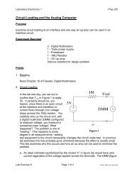
•Directions for hooking up your
solar cell
As a guide, look at the circuit diagram below. If
you have trouble connecting your circuit, ask
your lab instructor for assistance.
Luminosity
5) Back inside, calculate the power ouput of
your solar cell:
Power = Amps x Volts (6)
(Power = current x voltage)
6) This power of the solar cell is the M in equation
(5). Plug in your value and write the answer
here:
+ V
A
R
b o
= 10 x 10 x (1/A) x ______________
b o
= _______________
7) Now you’re ready to find your luminosity estimate.
Use equation (2) and your value of b o
above to calculate L o
L o
= 4πd 2 b o
= _______________
8) Compare your answer to the actual value of
about 4 x 10 26 W. What is your percentage error?
% error = (|actual-measured|/actual) x 100.
% error = _______________
9) Where do you think your error came in? How
could you measure the luminosity more correctly?
For credit, turn in your calculations, measured
values and answers to all questions
posed.
a) The symbol with the + sign refers to the solar
cell. It is your power source. Attach the red lead
from the solar cell to the mA (milliamp) setting
on your ammeter. An ammeter measures current.
The symbol A in the diagram above refers
to the ammeter.
b) The symbol R is the 1-Ohm resistor. Attach
the black (ground) ammeter connector to one
end of the resistor.
c) Attach the other end of the resistor to the
black lead from the solar cell.
d) V in the diagram refers to the voltmeter. A
voltmeter measures volts. Attach the two connectors
from the voltmeter, with the red connector
in the millivolt setting, one to each solar
cell lead.
e) Your circuit is now set up. Both meter’s black
connectors should be plugged into ground
(COM). If you have trouble getting a reading,
try checking the order of your circuit - you might
be registering negative values.
f) Remember when making your measurements
to convert from milliamps and millivolts back to
amps and volts.
10

•Materials
diffraction grating
helium lamp
oxygen lamp
hydrogen lamp
sodium lamp
mystery lamp
•Introduction
Spectra I
The figure below is an example of several spectra
from each stellar spectral class. In each
spectra, you can see not only what colors are
emitted, but also dark lines, called absorption
lines. The continuous spectrum is created by
the hot glowing gas in the low-lying levels of
the star’s atmosphere. The absorption lines are
created when this light flows outward through
the upper layers of the star’s atmosphere. Atoms
in these upper layers absorb radiation at
specific wavelengths, which depend on the specific
kinds of atoms present. Scientists group
stars with similar spectra into spectral classes.
Above or below the diagram, label the following
absorption lines:
1) Hα: red, strong in the mid spectral classes
2) He I: yellow, strong from O to K
3) Hβ: blue-green, strong from B5 to F5
4) Na I: yellow, strong in M
5) Hγ: blue, strong in B and A stars.
You may be wondering what the symbols α, β,
and I refer to. Hα is the symbol for hydrogen
alpha, the Balmer alpha electron transition for
hydrogen. Similarly for Hβ, only the Balmer beta
transition. Refer to your text for more information
on energy level transitions. I refers to the
fact that helium in this case is not ionized. He II
is helium that has lost one electron, Fe IX has
lost eight electrons, and so on.
A gas made of a certain element has its own
characteristic absorption lines. In this lab, you
will look at spectra from several gases, making
detailed observations of the lines. This will prepare
you for the next lab, Spectra II, where you
will actually analyze the spectra of some stars
and identify their chemical makeup by observing
their absorption lines.
•Procedure
1) Your lab instructor has several gas lamps,
one with helium gas, one with hydrogen gas,
one with oxygen gas, one with sodium gas, and
a mystery lamp (you have to guess what’s in
it). You will be given a diffraction grating, which
works like a prism, spreading out the wavelengths
of light. As the instructor turns on each
lamp, hold the diffraction grating to your eye so
you see a spread of colors. There are only two
orientations for the diffraction grating, one that
you will be able to see the bands and one you
won’t. Ask your lab instructor if you cannot make
out the bands. Write or draw your observations.
2) Although each lamp cannot be on for more
than about 30 seconds, your instructor will turn
on each lamp several times. Draw in the absorption
lines you see in the appropriate boxes
on the following page.
Spectra I
Copyright:
KPNO 0.9-m
telescope,
AURA, NOAO,
NSF
11

Hydrogen
blue
red
Spectra I
Helium
blue
red
Oxygen
blue
red
Sodium
blue
red
Mystery
blue
red
3) What is mystery lamp?
4) Turn in your observations for credit. Your
instructor will return them to you for the Spectra
II lab, where you will use them to help you
identify the absorption lines of the stars you
study.
12

Spectra II
O Star
1
O star spectrum
Spectra II
•Materials
text book, computers
•Introduction
In this lab, you will analyze at the actual spectra
of a few stars. Stellar spectra are the source
of almost all information we have about stars
and galaxies. See the Spectra I lab for more
information.
•Procedure
1) On this and the following page are spectra
from six different spectral classes of stars, O, B,
A, F, G, and K. You might want to refer to the
color table in the Herschel Experiment lab and
the image in Spectra I to help you associate
wavelengths with colors. By using the list of
absorption lines below and the descriptions of
the spectral classes, label the lines you see in
each graph. Remember, the symbol I after an
element indicates a neutral element, and II indicates
that the element is singly ionized (has
lost one electron). Hβ and Hγ are the Balmer
beta and gamma lines of hydrogen. Your lab
instructor will go through the first one with you.
Spectral classes:
O
B
A
F
G
K
M
Chemical
Name
Wavelength
(Angstroms)
Fe I 4303
Hγ 4340
He I 4386
He I 4470
He II 4685
Hβ 4860
He I 4920
[1 Angstrom = 10 -10 m]
- Ionized helium, weak hydrogen lines
- Helium and hydrogen lines
- Strong hydrogen lines
- weaker hydrogen lines than A stars,
Iron lines
- neutral metals, even weaker hydrogen
lines
- neutral metals
- molecules and metals
0.9
0.8
0.7
0.6
4200 4700 5200 5700
wavelength in Angstroms
B Star
A Star
violet blue green
B star spectrum
1
0.9
0.8
0.7
0.6
0.5
4200 4700 5200 5700
wavelength in Angstroms
A star spectrum
1
0.9
0.8
0.7
0.6
0.5
0.4
0.3
0.2
4200 4700 5200 5700
wavelength in Angstroms
13

F Star
1
0.9
0.8
F star spectrum
2) Turn on your computer. Open a web browser
and go to the following site:
http://stellar.phys.appstate.edu
Choose any star you’d like and save the data.
Open Excel, import the data, and make a plot
like the ones in this lab. If you need help doing
this, ask your lab instructor. What spectral lines
do you observe in your plot?
Spectra II
0.7
0.6
0.5
4200 4700 5200 5700
wavelength in Angstroms
•Questions
1) Which type of star is hotter, an O star or a G
star?
2) Why do stars have hydrogen and helium absorption
lines?
3) Why don’t the cooler stars have strong ionized
lines?
G Star
1
0.9
0.8
0.7
0.6
Solar spectrum
4) Why don’t the stars that are more hot have
metal lines? (Here, “metal” refers to any element
heavier than helium).
5) How could you tell, from this data, if a star
was moving relative to us?
6) What lines did you expect to see in the spectra,
but didn’t due to the fact that the spectra
stop at about 5600 Angstroms? Make a list below
for each spectral type, using your observations
from the Spectra I lab for hydrogen and
helium.
0.5
4200 4700 5200 5700
wavelength in Angstroms
O -
B -
A -
K Star
1
K star spectrum
F -
G -
K -
0.9
0.8
0.7
For credit, turn in your labeled spectra and
answers to the questions.
0.6
0.5
14
0.4
4200 4700 5200 5700
wavelength in Angstroms
Spectra obtained from data at
stellar.phys.appstate.edu

Size
the surface temperature and the luminosity. The
surface temperature is determined by the spectral
class. See the table below for the relationship
between surface temperature and spectral
class. Remember, an A1 star is hotter than an
A7 star.
Size
•Materials
Calculator
•Introduction
Stars, except the sun, are too far away to directly
measure their radius. Therefore, astronomers
use an indirect technique to estimate the
size of stars. In this lab, you will use this technique
to explore the variation of size in different
types of stars.
The Stefan-Boltzman law describes how much
energy is emitted per second per square meter
of a blackbody’s surface,
F = σT 4 , (1)
where F is energy flux, σ=5.67 x 10 -8 Wm -2 K -4 is
the Stefan-Boltzman constant, and T is the surface
temperature of the blackbody. This equation
applies very well to stars, whose spectra
are quite similar to that of a perfect blackbody.
A star’s luminosity is the amount of energy
emitted per second from its entire surface. In
the case of stars, we can safely assume a spherical
emission surface with area 4πR 2 , where R is
the radius of the star. The luminosity is therefore
L = 4πR 2 σT 4 . (2)
Since we are interested in finding the size of
stars, we would like an equation expressing R in
terms of the other variables. A useful way of
expressing the numbers in this kind of problem
is to use ratios referring to the sun. For the sun,
L o
= 4πR o2
σT o4
, (3)
where L o
= 3.8 x 10 26 W, R o
= 6.96 x 10 8 m, and
T o
= 5776 K. Dividing equation (2) by equation
(3) and solving for R/R o
, we get
R/R o
= (T o
/T) 2 (L/L o
) 1/2 . (4)
We now have the tool needed to calculate the
size of stars. In order to use this equation, we
need two pieces of information for each star:
To find the luminosity, we can use measurements
of the absolute magnitude, M. Absolute
magnitude is a quantity that describes the
brightness of a star (see the Luminosity lab)
and determines luminosity via the formula
M - M o
= 2.5 x Log(L/L o
). (5)
M o
is the absolute magnitude of the sun, and is
equal to +4.8. We want to know the luminosity
given the absolute magnitude, so we’ll rewrite
the equation in the form
L/L o
= 10 (Mo - M)/2.5 . (6)
Notice that there is not an absolute value sign
around (M o
- M). It is important to use the correct
sign for the star’s magnitude, M, as very
bright stars have negative absolute magnitudes.
•Procedure
Use equation (6), the table, and equation (4) to
find the radii in terms of the solar radius for
each star in the chart on the following page. To
get temperature, make an estimate given the
table above. For example, G2 star: (5900 K-
5200 K)/10 = 70 so G2 = 5900 K - 140 K =
5760 K. Fill in the blanks in the chart as you go.
Answer the questions in the section below.
•Questions
Spectral Class Temperature (K)
O 30,000 - 50,000
B 11,000 - 30,000
A 7,500 - 11,000
F 5,900 - 7,500
G 5,200 - 5,900
K 3,900 - 5,200
M 2,500 - 3,900
1) Are all of the stars in the chart that are hotter
than the sun bigger than the sun?
2) Are all of the stars in the chart that are more
luminous than the sun bigger than the sun?
15

Star
Spectral
Type
Temperature M L/L o R/R o
Alpha Centauri A
Arcturus
Betelgeuse
G2 4.4
K2 -0.3
M2 -5.6
Size
Capella
Deneb
G2 0.0
A2 -7.1
Proxima Centauri
Sirius
Spica
Vega
Wolf 359
M5 15.4
A1 1.5
B1 -2.0
A0 0.5
M6 16.7
3) Do all stars with the same luminosity have
the same size? Give an example.
4) Do all stars with the same temperature have
the same size? Give an example
5) What, if anything, strikes you about Betelgeuse?
What type of star do you think it is?
6) How does size vary with temperature (i.e. to
what power does size depend on temperature)?
How does size vary with luminosity?
7) According to equation (2), luminosity is related
to temperature. How so? Does this explain
your answer to question 5)?
For credit, turn in your calculations and answers
to all questions.
16

The H-R Diagram
•Materials
Computer Program: Microsoft Excel or
equivalent
•Introduction
The purpose of this lab is to give you a hands
(and computer) on experience with the
Hertzprung-Russell, or H-R diagram. A simple
review of its characteristics will be given. For
more information, please consult your textbook.
A basic knowledge of Microsoft Excel is helpful.
•Basics: the H-R diagram
The H-R diagram is a plot of the absolute magnitudes
of stars, M, versus their spectral type.
Sometimes you will see the y axis in units of
solar luminosity, L o
. Luminosity is directly proportional
to absolute magnitude, and in this lab,
we will use the absolute magnitudes of stars.
Remember, the more negative an absolute magnitude,
the BRIGHTER the star. We will also be
using the apparent magnitude, m, of stars. The
apparent magnitude refers to how bright a star
appears to us on Earth.
The x axis, spectral type, is a measure of a star’s
surface temperature. Astronomers label spectral
type with integers and letters, ranging from
M10 (cool, red), to O0 (hot, blue). Note that a
M7 type star is cooler than a M0 star, and that
the order of letters from cool to hot is: M, K, G,
F, A, B, O. The Sun is a G2 star with surface
temperature of about 5800 K.
•Basics: Luminosity classes
In addition to classifying stars into spectral
types, we group them into luminosity classes.
A star with the temperature 5800 K might be a
very luminous star (one with a negative value
of M), or a dim star (large, positive M). Astronomers
give groups of stars with similar luminosities
special names.
For example, the brightest stars are called luminous
supergiants and are labeled with the
luminosity class Ia. The Sun is a main sequence
star, class V. See the chart below for additional
information.
Luminosity Class
Ia
Ib
II
III
IV
V
Star Type
luminous supergiants
less luminous supergiants
bright giants
giants
subgiants
main sequence
•Basics: Plotting and using Excel
Here are some tips and hints for plotting your
data in Excel. The intent of these hints is not to
teach you how to use Excel. If you have questions,
see your instructor:
1) Convert your x axis values to numbers. For
example, set B=0, A=1, etc. Then you can use
G2=3.2, or K1=4.1, and so on.
2) In Excel, punch in your numbers for your x
and y axis.
3) Make a scatter plot, including axis labels.
4) To get the correct y axis, with negative values
at the top, click on the y axis in the plot
you’ve already created. Go to “Format”, “Selected
axis”, “Scale” tab. At the bottom, click
“values in reverse order.”
See your lab TA if you have questions.
•Create your H-R diagrams
A) Main Sequence Stars
Plot, in Excel or another graphing program, the
stars in Table A. The curve that approximately
connects these points is the main sequence;
most stars lie on this line. As mentioned earlier,
the main sequence stars are luminosity
class V stars. Make a label in your plot that
indicates this fact.
B) Giant Stars
Now plot the stars in Table B on the same
diagram. These are giant stars, luminosity
class III.
C) The Brightest stars in the sky
In a new diagram, plot all of the stars from Table
A and Table C. In Table C, the roman numerals
refer to the luminosity class, as in the table
above. “M” is absolute magnitude, and “m” is
apparent magnitude.
D) The Nearest stars in the sky
In another new diagram, plot all of the stars
in Table D.
The H-R Diagram
17

The H-R Diagram
Table A
Star Type M
Sun G2 +5.0
σ Per A B0 -3.7
γ Cet A2 +2.0
α Hyi F0 +2.9
Kruger 60B M6 +13.2
Procyon A F5 +2.7
61 Cyg A K5 +7.5
τ Cet G8 +5.7
α Gru B5 +0.3
Kapteyn's Star M0 +10.8
Table B
Star Type M
Arcturus K2 -0.3
Capella G2 +0.0
Aldebaran K5 -0.7
Pollux K0 +1.0
Table C
Star Type M m
Sirius A1V 1.5 -1.4
Canopus F0Ib -4.0 -0.7
Rigil Kentaurus G2V 4.4 -0.3
Arcturus K2III -0.3 -0.1
Vega A0V 0.5 0.0
Capella G2III 0.0 0.1
Rigel B8Ia -7.1 0.1
Procyon F5IV 2.7 0.4
Betelgeuse M2Ia -5.6 0.4
Achernar B5IV -3.0 0.5
Hadar B1II -3.0 0.6
Altair A7IV 2.3 0.8
Acrux B1IV -3.9 0.8
Aldebaran K5III -0.7 0.9
Antares M1Ib -3.0 0.9
Spica B1V -2.0 0.9
Pollux K0III 1.0 1.2
Fomalhaut A3V 2.0 1.2
Deneb A2Ia -7.1 1.3
Beta Crucis B0III -4.6 1.3
Regulus B7V -0.6 1.4
Adhara B2II -5.1 1.5
Castor A1V 0.9 1.6
Shaula B1V -3.3 1.6
Bellatrix B2III -2.0 1.6
Elnath B7III -3.2 1.7
Miaplacidus A0III -0.4 1.7
Alnilam B0Ia -6.8 1.7
18

Table D
Star Type M m
Sun G2 4.8 -26.8
Proxima Centauri M5 15.4 0.1
Alpha Centauri A G2 4.4 1.5
Alpha Centauri B K5 5.8 11.0
Barnard's Star M5 13.2 9.5
Wolf 359 M6 16.7 13.5
Lalande 21185 M2 10.5 7.5
Sirius A A1 1.5 -1.4
Luyten 726-8A M6 15.3 12.5
Luyten 726-8B M6 15.8 13.0
Ross 154 M5 13.3 10.6
Epsilon Eridani K2 6.1 3.7
Luyten 789-6 M6 14.6 12.2
Ross 128 M5 13.5 11.1
61 Cygni A K5 7.5 5.2
61 Cygni B K7 8.3 6.0
Epsilon Indi K5 7.0 4.7
Procyon A F5 2.7 0.3
Cincinnati 2456A M4 11.2 8.9
Cincinnati 2456B M4 12.0 9.7
Groombridge 34A M1 10.4 8.1
Groombridge 34B M6 13.3 11.0
Lacaille 9352 M2 9.6 7.4
Tau Ceti G8 5.7 3.5
Luyten's Star M4 11.9 9.8
Lacaille 8760 M1 8.8 6.7
Kapteyn's Star M0 10.8 8.8
Kruger 60A M4 11.7 9.7
Kruger 60B M6 13.2 11.2
•Questions
Answer the following questions on a separate
piece of paper. For credit, turn your answers
and your plots.
1. Why don’t the stars in Table B lie on the curve
you created in part A) ?
2. How many magnitudes is Capella brighter
than the Sun?
3. How many times brighter is Capella than the
Sun?
4. Is Capella larger or smaller than the Sun?
5. What is the most common kind of bright (M)
star (hot, cool, or spectral type)?
6. Estimate the average apparent magnitude,
m, of the brightest stars (Table C).
7. When you look at a bright star in the sky,
your probably looking at what speectral type of
star?
8. What is the most common kind of star near
the Sun?
9. Estimate the average apparent magnitude
of the close stars (Table D).
10. We believe the stars near the sun are ordinary,
common stars. Why don’t we see mostly
common stars?
11. What would our night sky look like if all the
stars in the galaxy had the same absolute magnitude
as the Sun?
12. Write a short summary of what you learned
in the lab.
The H-R Diagram
19

Herschel Experiment
The Herschel
Experiment
•Materials
One glass prism
3 alcohol thermometers with blackened bulbs
scissors
cardboard box
blank piece of white paper
•Introduction
Herschel discovered the existence of infrared
light by passing sunlight through a glass prism
in an experiment similar to the one you’ll do
here. As sunlight passed through the prism, it
was dispersed into a rainbow of colors, a spectrum.
Herschel was interested in measuring the
amount of heat in each color and used thermometers
with blackened bulbs to measure the
various color temperatures. He noticed that the
temperature increased from the blue to the red
part of the visible spectrum. He then placed a
thermometer just beyond the red part of the
spectrum in a region where there was no visible
light and found that the temperature was even
higher. Herschel realized that there must be
another type of light beyond the red, which we
cannot see. This type of light became known as
infrared. Infra is derived from the Latin work for
“below”. In this lab, you will complete an experiment
very similar to Herschel’s original one.
•Predictions
Before starting the experiment, make some predictions
about what will happen. Write answers
to the following questions on a piece of paper
that you will hand in with your lab. It’s okay if
you don’t know the answer right now, but put
down your ideas anyway. In what region will
you observe the highest temperature? Why?
What color is the sun? Why to we see in “visible”?
What kind of light is more energetic, red
light or blue?
•Procedure
This experiment should be conducted outdoors
on a sunny day.
1) Place the piece of white paper on the bottom
of the cardboard box.
2) Carefully attach the glass prism near the top,
sun-facing edge of the box. Do this by cutting
out an area from the top edge of the box that
the prism will fit snugly into.
3) Place the prism in the slot you created and
rotate it so it creates the widest possible spectrum
on the shaded portion of the white sheet
of paper at the bottom of the box. You can elevate
the sun facing side of the box to create a
wider spectrum.
4) Now, place the three thermometers in the
shade and record the temperature each reads.
5) Next, place the thermometers in the spectrum
such that one of the bulbs is in the green
region, another in the orange region, and the
third just beyond the red region. If you can’t
get this to work out perfectly, that’s okay, just
make sure to record what region each of your
bulbs was in during the time you took your
measurements.
6) It will take 3 minutes or so for the thermometers
to record the final values. Do not move the
thermometers from the spectrum or block the
spectrum while reading the temperatures.
7) Record all of your measurements on a piece
of paper that you will turn in with the rest of
your lab. You should record the temperature of
each thermometer after each of the three minutes.
8) Repeat steps 4-7 two more times.
9) Calculate an average final temperature for
each region and record. Compare your averages
with the other lab teams.
•Questions
Answer the following questions on a separate
piece of paper. For credit, turn your answers,
your predictions, and your recorded data.
20

1) What color/region did you find to have the
highest temperature? Did you measure infrared
light? Did you record different values during different
runs?
2) Does it make sense to you what region had
the peak temperature? In what color do you
think the sun emits the most energy?
3) Look at the following diagrams and corresponding
discussions, then re-analyze your answer
to question 2.
4) Answer all questions posed in the discussion.
List of visible wavelength ranges, for reference.
Red
620-700nm
Orange 590-620
Yellow 570-590
Green 490-570
Blue 440-490
Violet 390-440
There are 10 9 nanometers (nm) in a meter.
Planck spectrum 5770K
2´ 10 -7 4´ 10 -7 6´ 10 -7 8´ 10 -7 1
Wavelength in meters
You should recognize this plot as a Planck or
blackbody spectrum. The radiated light from
the sun can be approximated by a blackbody
at 5770K. Use Wien’s Law to find the peak
wavelength of the Sun’s emission.
Wien’s Law:
Herschel Experiment
To change a wavelength into a frequency, use
the formula
ln = 3*10 8 m/s
where n is frequency in Hz and l is wavelength
in meters.
index of refraction
1.55
1.54
1.53
1.52
1.51
1.5
1.49
1.48
1.47
1.46
Variation of index of refraction for
glass
1.45
200 300 400 500 600 700
wavelength in nm
The graph above is plot of how the index of
refraction varies with wavelength in glass. There
are actually many types of glass, and each has
a somewhat different index of refraction. This
one is for silica. If the plot were a straight line,
“linear”, we would have equal spacing of wavelengths
when light is refracted through a prism.
However, the plot is not a line, but a curve which
flattens out toward the red end of the spectrum.
Due to the fact that the index of refraction
changes very little at the red end of the
plot, the wavelengths there will be bunched up,
more concentrated.
l max
= 2.9*10 6 /T
Where l max
is the peak wavelength of the
Planck spectrum in nanometers and T is
temperature in Kelvin.
Is this the wavelength you expected? To obtain
an energy from the Planck spectrum, integrate
over a wavelength range. If you are unfamiliar
with the concept of integration, you can think of
it here as the area under the curve from one
spot on the x axis to another. For example, you
can see by simply looking at the plot that the
area under the curve between 200 and 300 nm
is less than the area between 500 and 600 nm.
Using this type of estimation, in which color does
the sun emit the most energy? The difference
between energy emitted from the sun in green
and red is not great, but in a well done, corrected
experiment, is measurable.
You might now be asking yourself a logical question.
If the sun emits the most in green, why
does it appear yellow? In fact, it is an appearance.
The sun is actually white, but against the
blue sky, it looks yellow. Caution: never look
directly at the sun - it can burn your eyes in a
matter of only a fraction of a second. Astronauts
in space observe the sun as white, due to the
black rather than blue background they see it
against. To prove this to yourself, try the following
experiment on your own time.
21

Herschel Experiment
Experiment:
Gather two pieces of blue paper and a small
square of white paper. Attach the white square
to the middle of one of the sheets of blue paper.
Stare at the empty blue page for about 30 seconds,
then place the other on top. What color do
you observe the white paper to be? Most see the
white chunk as yellowish!
It is a common misconception that the sun is
yellow. In fact, most astronomy text books simply
classify the Sun as a G2 “yellow” star and
don’t explain the difference between the spectral
classification and the true “color” of the Sun
or other stars. Of course, we could spend quite
a bit of time discussing what exactly color is,
and how our eyes see color, but that is left to
you. The following website is helpful if you’re
interested:
http://casa/colorado.edu/~ajsh/colour/
Tspectrum.html
5) Summarize what your Herschel experiment
results were, why you got those results, and
state what you should have observed if you corrected
for the non-linear nature of the index of
refraction of glass.
•Further investigaion (for extra
credit)
The formula for Planck function is
B l
(T) = (2hc 2 /l 5 )(exp(hc/klT)-1) -1
Where
h = Planck’s constant
= 6.626*10 -34 J*s
c = speed of light
= 3*10 -8 m/s
k = Boltzman’s constant
= 1.38*10 -23 J/K
Use T = 5770K for the temperature of the Sun.
Using Mathematica or some other math tool,
plot the function. Then numerically integrate
over a few wavelength ranges to obtain the energy
emitted in that range. What percent of visible
light energy is green? Red?
22

Solar Observation
•Materials
Telescope operating instructions
Sun chart
Telescope
Filters
•Introduction
In this lab, you will use the department’s 8 inch
telescopes and two types of solar filters. NEVER
LOOK DIRECTLY AT THE SUN! The sun can
burn your eyes in a very short period of time,
resulting in permanent damage. Astronomers
use special filters to filter out the powerful radiation
of the sun so we can safely observe it.
The filters are placed on the telescopes before
pointing them at the sun, because the sun can
also damage the optics inside the telescope.
Your lab instructor will set up the telescopes for
you, so you don’t need to worry about placing
the filters correctly. You should, however, know
the difference between the filters and how to
operate the telescope while you’re observing.
Refer to the telescope operating instructions at
the front of this manual for information on the
latter.
The first of two types of solar filters you’ll be
using in this lab is a neutral density or white
light filter. A white light filter blocks out all types
of light equally. Usually, they are made of mylar.
When you look at the sun through this type of
filter, you will see the surface of the sun. The
surface is the layer where the visible light, produced
in the center of the star, is released. It is
no mistake that we see in “visible”; this is the
range of light that is emitted more than any
other from the sun. Solar physicsits call the
surface layer the photosphere. Often, the
photosphere has large dark patches, sunspots,
that rotate with the sun. Sunspots are regions
of concentrated magnetic field. They appear dark
because they are about 1500 K cooler than the
surrounding “quiet” photosphere, at 5800 K.
Cooler temeratures in sunspots are a result of
the strong magnetic field suppressing the convection
that continually brings up hotter material
from under the surface. In the quiet photosphere,
the convection results in granulation
cells. You won’t be able to observe the granulation
cells with the telescopes we have, but take
a look at the following web site to see some
amazing images of granulation and sunspots.
http://www.solarview.com/eng/sunspot.htm
You will be able to see sunspots well. That is, if
there are any to be seen! The sun has an eleven
year activity cycle, and sun spot number is a
good indicator of activity. At solar maximum,
there will likely be as many as 100 sunspots
visible from Earth. During minimum, chances
are there will be only a couple or even none. The
last solar max was around 2000-2002. Solar
minimum is expected to last from about 2004-
2009. People have been charting sunspots for
hundreds of years, since Galilleo. Look at the
diagram below and make a guess yourself as to
when the next solar max will take place.
Monthly Average Sunspot Number
The second type of filter you will observe with is
an Ha (said “H alpha”) filter. Ha refers to the
Balmer alpha transition for the Hydrogen atom.
(See the section of your textbook on spectral
lines for more information.) The wavelength of
Ha is 656 nanometers, corresponding to a red
color. Through a telescope with an Ha filter on
it, you will see the area of the sun’s atmosphere
that emits in Ha, the chromosphere. The chromosphere
lies just above the photosphere, and
is about 10,000 K. You will still see sunspots,
but you should also be able to see prominences.
A prominence is a region of dense, relatively
cool plasma suspended in the hot corona (the
outermost part of the solar atmosphere) . These
mysterious phenomena are at chromospheric
temperatures even though they reside in the
million degree corona. Again, for more information,
see your text. Look for prominences just
off the limb (edge) of the sun. They will appear
as reddish blurs against the dark background.
Solar Observation
23

Solar Observation
•Procedure
1) Read telescope operating instructions located
in the front of the manual.
2) Look at the following two websites for information
on what the sun currently looks like.
Make some notes about how many sunspots are
on the solar disk and where they’re located. Do
you see any prominences in the Big Bear Solar
Observatory’s Ha image? If so, where are they
in respect to the sunspots?
http://www.spaceweather.com
http://www.bbso.njit.edu/cgi-bin/LatestImages
3) After your lab instructor has set up a filtered
telescope for you, position the telescope so it is
pointing at the sun. Important note: make
sure the viewfinder scope is covered. The easiest
way to position the scope the correctly is to
minimize the shadow cast by the scope. Then
look through the main eyepiece. If the sun is
not visible, try again. It is best to start with a
wide angle eyepiece (40 mm). Once you have
the sun in your field of view, you can zoom in by
replacing the 40 mm eyepiece with a 20 or 25
mm one.
Trace the chart onto a piece of paper or get a
copy of the chart from your lab instructor.
For credit, turn in your notes from surfing
the solar websites and your solar observations.
•Further investigaion (for extra
credit)
The rotation of the sun is easily observed by
plotting sunspot location over a series of days.
Your lab instructor can set up a time for you to
do a quick solar observation several days in a
row. Carefully draw what you see each day. What
do you guess the rotation period of the sun to
be?
4) Make drawings of sunspots and prominences
on the solar chart. Label the date, time, type of
telescope, filter, and eyepiece type. Note that
the telescope flips the image upside down and
backwards. Which way is solar north? Think about
this carefully!
24
Sun
Chart

•Materials
Stellar Structure
Computer program: Microsoft Excel or Equivalent
•Introduction
When you think of a star, what properties do
you associate with it? It’s a hot ball of gas, right?
What about that hot ball of gas makes it a star?
A good answer to this question is that a star is
stable. Our Sun, for example, is not exploding
or contracting. Scientists refer to the stability of
stars by saying that they are in hydrostatic
and thermal equilibrium. Hydrostatic equilibrium
is a balance between the forces that act on
the star. The forces include downward pressure
of the gas layers into the center, upward pressure
of the hot gasses, and the downward pull
of gravity due to the weight of the gas itself.
The upward gas pressure must compensate for
both gravity and the pressure of the outer layers.
Thermal equilibrium means that even
though the temperature in stellar interiors varies
with depth, the temperature at each depth
remains constant in time.
Another important property of a star is how
energy is transported from its center to the surface.
The energy source for stars is the nuclear
reactions that take place in the core. The energy
is transported to the surface by conduction,
convection, and/or radiative diffusion. In
the sun, energy is transported by radiative diffusion
from the core to about 0.7 solar radii.
From that depth out, energy is transported by
convection. Some stars have very large radiative
zones and little or no convective zones, while
others have very deep convective zones.
Scientists use equilibrium concepts, along with
energy transport mechanisms, to construct
models for stellar structure. The models determine
the size, temperature, and mass of the
star. Some stars are very large and luminous,
but cool. Others are small but very hot. The sun
is a main sequence, or hydrogen burning, star.
In this lab, you will study the relationship between
luminosity and three factors: temperature,
mass, and radius of main sequence stars.
•Procedure
In this lab, you will take a close look at how
three aspects of stellar structure (temperature,
mass, and size) effect luminosity. Scientists often
use luminosity to learn about stellar structure
because it is easily measured, and many
other informative quantities can be deduced from
it. You will look specifically at main sequence
stars, which generally obey the following equations:
1) L/L o
= (T/T o
) 6
2) L/L o
= (M/M o
) 4
3) R/R o
= (M/M o
) 0.7
where L = luminosity, T = temperature, M =
mass, R = radius, and the subscript o
refers to
the solar value for that variable.
*How is luminosity related to radius?
4) L/L o
= ___________
Use equations 1, 2 and 4 to fill out an Excel
table. If you are unfamiliar with doing math in
Excel, see the instructions on the next page.
You will use logarithmic x and y values to
make a plot of the three luminosity relationships
in Excel. The x axis will always have
the same values, referring to T/T o
for the
first relationship, M/M o
for the second, and
R/R o
for the last. Calculate the y axis values
using the appropriate equation: (T/T o
) 6 for the
first, etc., then take the logarithm of these values.
Once you’ve made all of your calculations,
create a plot in Excel. Excel hint: when plotting
this type of data, use the scatter plot that creates
a line through the data points. Ask your lab
instructor if you have questions on how to create
the plot. For credit, turn in your (x,y) values,
plot and answers to the questions below.
•Questions
1) What aspect of solar structure increases the
luminosity the most as it increases? The least?
2) Why is it better to plot the logarithm of the
values you calculated rather that the actual values?
3) The plot of L/L o
vs. T/T o
is the usual way you
will see a Hertzprung-Russell diagram displayed.
Why is it a straight line instead of a curve? Hint:
look at the procedure you followed in the H-R
diagram lab compared to this lab.
Stellar Structure
25

Stellar Structure
Using Excel to do math
1) In Excel, create a column title for each of the
columns in the chart below. In column A, enter
the x axis values (0.1, 0.25, etc.).
2) Click on the box in column B that has the x
value 0.1. Go to Insert -> Function -> Math and
Trig -> select LOG10. Click “okay”. When the
box comes up asking for a number, click on the
box in column A with the value 0.1. Click “okay”.
3) Now select the box just created in column B
(value=-1, log base 10 of 0.1) and Edit -> Copy.
Next, highlight the rest of column B and Edit -
> Paste. You now have the logarithmic numbers
corresponding to the values in column A.
4) Now, we need to find luminosity for the temperature
ratio, which goes to the 6 th power. When
the first empty box in column C is highlighted,
go to Insert -> Function -> Math and Trig ->
Power. Click “okay”. In the box that comes up,
put 6 as the power, click the box with the value
0.1 in column A, and click “okay”. Copy and
paste for the rest of column C as before. Create
logarithmic values of column C in column D as
you did for the x values.
5) Repeat step 4) for the other luminosity relationships.
Once done, either copy the values
from Excel into your notebook, or print off
a copy of the Excel workbook to attach with
your lab.
6) Now, plot the three log/log luminosity relationships
on the same chart. Highlight columns
B, D, F, and H by using ctrl + click to select
multiple columns. Go to Insert -> Chart -> XY
scatter and choose the chart with the dots and
the line through them. Each relationship will be
a different color. Name the “series” in the first
box that comes up when inserting the chart.
A B C D E F G H
X Axis values L/L. = (T/T.)^6 L/L. = (M/M.)^4 L/L. = (R/R.)^(4/0.7)
X/X. Log(X/X.) L/L. Log(L/L.) L/L. Log(L/L.) L/L. Log(L/L.)
0.1
0.25
0.5
0.75
1
1.5
2
2.5
3
3.5
4
4.5
5
10
26
For reference:
L o
= 3.86 x 10 26 W, T o
= 5776 K, M o
= 2 x 10 30 kg, R o
= 7 x 10 8 m

Stellar Evolution
This is a good lab to do on your own if you have
missed a lab class.
Your parents hear on TV that one day, the Sun
will grow into a huge, red ball of gas extending
all the way to Earth. They know you’re in an
astronomy class and call you up to ask if this is
true. Write a phone conversation you would have
with them, explaining in laymen’s terms the
birth and death of stars similar to the sun.
Stellar Evolution
For extra credit, explain how larger and smaller
stars’ evolution varies from the evolution of stars
the size of the sun.
Alternative:
If you like to draw, create an image for each
step of the stellar evolution progress. Include a
short statement of explanation with each drawing.
A picture is worth a thousand words! The
same extra credit applies, only with drawings
and a short statement rather than in writing.
27

Neutron Stars
•Materials
•Introduction
Neutron Stars
Iron filing demonstration
In this lab, you will explore the properties of
several types of neutron stars. First, your lab
instructor will introduce the concept of magnetic
field using a bar magnet and iron filings.
Study the chart below for an understanding of
magnetic field strengths.
Magnetic Field
magnitude (Gauss)
Object
0.6 Earth's field
100
common hand held
magnets
4000 strong sunspots
4.5 x 10 5 strongest sustained
magnets*
1 x 10 8 strongest nonneutron
star fields
10 12 - 10 13 radio pulsars
10 14 - 10 15 magnetars
*If made any stronger, the magnet would exceed the tensile
strength of the material, and it will blow apart!
Gamma-ray bursts (GRBs) were first detected
in the late 1960s by U.S. satellites designed to
look for space-based nuclear weapons testing.
GRBs are characterized by a short burst of
gamma rays (from milliseconds in duration to a
few minutes), and rarely have an easily detectable
glow more than a few minutes after the
event. GRBs are flashes-in-the-pan: they explode
once, never to return.
GRBs were a big mystery to astronomers when
they were first seen (and in fact, they still are).
The situation became worse when, on March 5th,
1979, intense flashes of gamma rays were detected
coming from the direction of the Large
Magellanic Cloud, a companion galaxy to the
Milky Way. Then, over the next few months, more
flashes of gamma rays were detected coming
from the same region of the sky. For a while, the
idea that GRBs only flashed once was in doubt,
but then it was realized that the repeating
sources were a totally different class of object.
Dubbed Soft Gamma Ray Repeaters (SGRs),
because they peak at a slightly lower (also called
“softer”) energy of gamma ray than GRBs, these
were found to be neutron stars - incredibly dense
remnants of supernova explosions - which have
extremely strong magnetic fields, far stronger
than typical neutron stars. For reasons still unknown,
the super-magnetic field can cause the
crust of the neutron star to slip, much like an
earthquake. The intense gravity of the neutron
star makes such a slip a dramatic event indeed;
the energies can be enough to generate huge
bursts of gamma rays which typically last for
less than a second. Over time, the pressure
builds up again, and another flash is seen. This
is how gamma rays are seen from the same
object more than once.
Also in the mid-1970s, different kinds of highenergy
events were starting to be identified.
The so-called X-Ray Bursters (XRBs) were discovered.
Like SGRs, they were neutron stars with
repeating bursts, but their magnetic fields, while
strong, were not at the level of the SGRs’
strength. And unlike SGRs, which are isolated,
individual neutrons stars, XRBs are caused by
neutron stars in binary systems. The neutron
star in such a system can accrete, or draw in,
matter from a normal companion star. The matter
builds up on the surface of the neutron star,
and then suddenly explodes in a thermonuclear
blast. It is this explosion which creates the burst
of X-rays, which lasts for roughly 20 to 100 seconds.
After the matter burns up in the blast, the
accretion starts again and the pattern repeats.
This causes repeated XRBs from the same object.
During the 1970s through the 1990s, much
confusion arose because it was not clear at first
that there were actually three different types of
physical mechanisms that were producing the
bursts of energy. Placing something in its correct
category is half the battle in understanding
it. It took 30 years for astronomers to sort out
these different types of phenomena, and in fact
they are still working on classifying and understanding
them. You will do the same, but in just
45 minutes or so!
28

•Procedure
1) You will use the data given in the table on the
following page to make deductions about any
trends in the objects and determine how many
categories (based on common properties) there
are from those trends. You need to decide which
objects belong to which categories.
Data types:
Object name. The name of the object is based
on its coordinates on the sky. The sky is mapped
by astronomers using a coordinate system similar
to longitude and latitude, but the axes are
called Right Ascension (or RA) and declination.
RA is measured in the direction of East-West on
the sky, and goes from 0 to 24 hours (each further
divided into 60 minutes). Declination is
measured in North-South on the sky, and goes
from -90 to 90 degrees. An object’s name on
the card is its RA (a four digit number where the
first two digits are the hours, and the second
two are the minutes) and its declination in degrees,
including the plus or minus sign. An object
at an RA of 5 hours 30 minutes and a declination
of -20 degrees would this have the name
0530-20.
2) Using the location data (galactic coordinates),
plot the distribution of the mystery objects in
the sky. Make a copy or trace the projection map
at the end of the lab, then plot each of the objects
on that separate page. Use a different symbol
for each group from part 1.
•Questions
1) How many groups do you think there are?
What properties do you think are the most useful
for separating the groups?
2) What can you say about the distribution of
each group on the map? Are the bursts in each
group randomly located, or do they fall into a
pattern on the sky?
3) What is the average peak energy of the bursts
in each group?
4) What is the average distance from the Earth
of the bursts in each group? Is there a lot of
variation in the distances of the objects in each
group, or are they all about the same distance?
Neutron Stars
Location. Latitude (b) and longitude (l) in Galactic
coordinates of each burst.
Energy Peak. The energy where the burst has
the maximum number of photons.
Optical Counterpart. What is seen in visible
light at the position of the burst.
Distance. The distance from the Earth to the
burst in light years.
Burst Repetition. How often the bursts are seen
to recur, if they do recur. “None” means that no
repetition has been detected, and “N/A” means
no information is available.
Spin or Orbital Period. Either the spin period
of the burster, or its binary orbital period if it is
in a binary system.
5) What other properties do the members of
each group have in common?
For credit, turn in your map and answers to
the questions above and below.
•Further investigation (required)
www.nasa.gov/vision/universe/watchtheskies/
swift_nsu_0205.html
Explore the December 27, 2004 event on the
website above and answer these questions:
1) According to your work in part 1 of the lab,
what type of burst was this? What caused the
burst? How far away was it? What special name
is given to this type of neutron star?
2) How much more powerful was it than previous
record holders? How long would it take the
sun to produce this much energy?
29

Neutron Stars
Name
Location
(l,b)
Energy
Peak (keV) Optical Counterpart
Distance
(light years)
Burst
Repetition
Spin or Orbital
Period
0501+11 189, -18 175 Mag 25 host galaxy 5.7 billion none none
0526-66 276, -33 30 Super nova remnant 180,000

Cosmology: The
Expansion of the
Universe
•Materials
one balloon per person
string
rulers
•Introduction
In this exercise, you will use a two-dimensional
model to explore the expansion of the universe.
Before 1917, many scientists thought the universe
always existed. But Einstein’s revolutionary
theory of gravity changed all the rules. It
opened up the mind-boggling possibility that
space itself - the permanence of which had never
been questioned - might actually be expanding.
If space is expanding, the universe we inhabit
today could once have been infinitely
smaller.
In 1929, astronomer Edwin Hubble made the
amazing discovery that distant galaxies are
speeding away from us. This means that the
galaxies we see today were once much closer
together - originating from a tiny region of
space.
The origin of the universe remains one of the
greatest questions in science. Current scientific
evidence supports the Big Bang model, which
states that about 13.7 billion years ago, the
entire universe began expanding from a very
hot, dense state. This sudden expansion is know
as the Big Bang.
What does it mean to say that the universe is
expanding? The Big Bang was an expansion of
space itself. Every part of space participated in
it. Space is not simply emptiness; it’s a real,
stretchable, flexible thing. Galaxies are moving
away from us because space is expanding. Galaxies
are moving with space, not through space.
(There is also a local motion through space as
galaxies interact with their neighbors, but on
larger scales, the expansion of space dominates.)
The model in this activity demonstrates
how the motions of the galaxies reveal the continuing
expansion of the universe.
In the 1920s, Edwin Hubble measured the motion
of the galaxies. By measuring a galaxy’s
distance from us and how fast that galaxy is
receding (its recession velocity), he found a
simple relationship: double the distance, double
the velocity; triple the distance, triple the velocity.
This is Hubble’s Law. In equation form,
it is written:
v = H x d
Recession velocity = Hubble’s constant x distance from us
The slope of the graph of distance vs. velocity
represents the Hubble Constant for the universe.
The Hubble Constant describes how fast the
universe is expanding. By measuring the rate of
expansion, the size and age of the universe can
be calculated. Interpreting recent observational
results from space-borne and ground-based
telescopes, scientists have determined different
values of Hubble’s constant. Determining
the precise value of the Hubble constant is key
to understanding the origin of the universe, and
there are several factors that affect this determination.
For example, the universe may not
have been expanding at the same rate throughout
time; that is, the expansion itself may be
accelerating. Questions like these make the age
of the universe a hot topic - one of the most
controversial in the study of cosmology. The age
of the universe is currently estimated to be about
13.7 billion years, and the Hubble constant is
estimated to be about 70 km/s/Mpc.
The age of the universe can be calculated from
the Hubble constant; it is its reciprocal. However,
this assumes that the universe expands at
a constant rate, and that may not be accurate.
•Procedure
1) Blow up the balloon a little bit. DO NOT TIE
IT SHUT!
2) Draw and number ten galaxies on the balloon.
Mark one of these galaxies as the reference
galaxy.
3) Measure the distance between the reference
galaxy and each of the numbered galaxies. The
easiest way to do this is to use a piece of string.
Stretch it between the two points on the balloon,
then measure the string. Record these data
in the table. Be sure to indicate the units you
are using.
4) Now blow up the balloon. You can tie it shut
this time if you like.
5) Measure the distance between the reference
galaxy and each of the numbered galaxies.
Record these data in the table.
Expansion of the Universe
31

Expansion of the Universe
Galaxy
Number
First
Measurement
Second
Measurement Difference Velocity
Velocity
32
Distance
6) Subtract the first measurement from the
second measurement, record the difference in
the data table.
7) Estimate the amount of time it took you to
blow up the balloon (in seconds). Divide the
distance traveled (the difference) by this time
to get a velocity.
8) Plot velocity versus the second measurement
to get the “Hubble Law for Balloons”. Don’t forget
to label the units on your axes.
9) Fit a line to your data.
10) Find the slope. Slope is the change in y over
the change in x. This is exactly the way that we
find the value of Hubble’s Constant from
Hubble’s Law.
11) Find the age of your balloon universe from
this slope. Remember that the age is one over
the Hubble Constant.
•Questions
1) How does the age of the balloon found from
the Hubble law compare to the time it took you
to blow up the balloon the second time?
2) What assumptions do you make about your
balloon universe when you find it’s age by this
method? Are these sensible assumptions?
3) How would your results change if you used a
different reference “galaxy” on the balloon? If
you are not sure, try it!

Planets Outside Our
Solar System: Is there
life on other worlds?
The Drake Equation
•Materials
calculator
•Introduction
Are we alone? For the first time in history, astronomers
have discovered planets orbiting stars
beyond our own Sun. In fact, planetary systems
seem to be widespread in the universe. Is
there life, intelligent or otherwise, in any of these
alien solar systems? No one yet knows. But ours
may be the first generation to detect a sign of
life beyond Earth. What will it mean if we find
out that we are not alone?
At first, “Is there life on other worlds?” seems a
simple question to answer. However, it quickly
becomes a complex web of issues. What is life,
anyway? How does it begin and evolve? What
conditions can life tolerate? What makes a planet
habitable? How do we look for and identify extraterrestrial
life? To attempt to resolve these
kinds of questions, astrobiologists draw on many
branches of science and employ many research
strategies, such as fieldwork, laboratory research,
telescopic observation, and exploration
with spacecraft.
Though we have not found any examples of
extraterrestrial life, comparisons with certain
kinds of life on Earth suggest that potential habitats
for extraterrestrial life, and maybe life itself,
do indeed exist. However, contrary to popular
notions, if extraterrestrial life is found in our
solar system, it will most likely be bacteria-like.
In 1961, the astronomer Dr. Frank Drake suggested
an organized framework for thinking
about life in the galaxy. Known as the Drake
Equation, it provides a way to estimate the number
of worlds within our Milky Way galaxy that
have intelligent life and whose radio transmission
should be detectable. Drake identified a
sequence of eight terms to help people think
about what must occur before a world can be
inhabited by a civilization with radio technology.
This activity uses Dr. Drake’s framework to
have you consider the implications of each term
and make your own estimates of life in the Milky
Way galaxy.
Because we are unsure whether there is life out
there, let alone intelligent life with which we
can communicate, there is no correct solution
to the equation - the value of each factor is
open to interpretation.
•Procedure
To find out your estimate of the number of worlds
in the Milky Way galaxy that have intelligent life
that we can detect using radio technology, fill
out the chart on the following page. Multiply the
eight terms. Don’t forget to convert percentages
to numbers.
•Questions
1) What is your final answer?
2) Based on your estimates, how good are our
chances of hearing from intelligent extraterrestrials?
3) How does your answer to 2) compare with
what you thought before you began the activity?
4) What if you answer to 1) were less than one?
What would that mean in terms of our existence
here on Earth?
5) When making estimates, in which terms did
you have the most confidence? The least? Why?
6) Are you more optimistic or more conservative
when it comes to thinking about extraterrestrial
life with radio technology in the Milky
Way galaxy? Why?
7) How could you adjust the estimates in the
equation to have it come out so that Earth is the
only planet in the Milky Way galaxy with radio
technology?
8) What would your reaction be if we discovered
microbes on another planet? Plants? Insects?
Mammals? Intelligent life?
9) If microbial life were discovered on another
planet, what implications might the discovery
have?
Life on other worls?
33

Life on other worlds?
Term
Background
1. The total number of These numbers are based on observations of the stars in our
stars in the Milky Way galaxy and of other galaxies we believe to be like our own.
Galaxy
Most scientists believe the number of stars to be 400 billion.
2. The percentage of
stars that are
appropriate
3. The average number
of planets around
each appropriate star
4. The percentage of
planets within a solar
system that are
habitable
5. The percentage of
habitable planets that
develop life
Many scientists believe that a star has to be like our Sun. Only
about 5% of the stars in our galaxy are sun-like stars, though
about 10% are closely related, either slightly warmer or slightly
cooler. About 50% of stars exist in binary or multiple systems,
which many scientists feel make them inappropriate.
Appropriate stars may not have planets circling them. We have
only just begun detecting extra-solar planets, so we don't really
know how common they are.
Our only example of this term is our own solar system. Could
Earth be the only habitable place in our solar system? Is our
system typical? Remember that if one system has no habitable
planets and another has four, the average would be two per
system.
Having a planet that is appropriate for life doesn't necessarily
mean that life will arise. No real data are available to help us
estimate this term. Earth is the only planet on which we know
there is life. However, bacterial life existed on Earth shortly
(geologically speaking) after its formation, possibly indicating
that the development of life is easy. Many scientists believe that
whether or not life arises depends on many factors.
Conservative Optimistic
Estimate Estimate
100 billion 600 billion
0.05% 45%
1 10
10% On
average, there is
one habitable
planet in every
system
0.000001% Life
is a rare accident
that is unlikely
to happen
elsewhere
50% Half the
planets in are
habitable
100% Life will
arise if
conditions are
approprite
Your Estimate
6. The percentage of On Earth, humans developed intelligence, aparently as an
planets with life that evolutionary advantage. However, this term depends on how
develop intelligent life
you define intelligence. Are dolphins, gorillas, octopus, and ants
intelligent? Furthermore, single-celled life existed on Earth very
early, and multicellular life took 2.5 billion years to form (a very
long time, geologically speaking). Maybe the development of
complex life, let alone intelligent life, is unusual.
0.0001% or less
Only one in a
million planets
with life will
devolop
intelligent life
100% Any
planet with life
will develop
intelligent life
7. The percentage of
intelligent life that
develops radio
technology
8. The percentage of
"current" civilizations
having radio
technologies
Communication with intelligent extraterrestrials requires that
we hear from them. Given the vast distances of space, they
would probably send signals that travel at the speed of light,
such as radio waves. On Earth, humans have only just
developed radio technology, so possibly this term should have
a low value. But, we did eventually develop radio technology,
so maybe this is true of all intelligent beings.
Will an extraterrestrial's signals overlap with the lifespan of the
receiving civilization? Extraterrestrials that sent signals a
hundred thousand years ago from a world a hundred thousand
light years away would still overlap with us, even if they died
out long ago. So, how long do civilizations with radio
technology last? A high level of technological development
could bring with it conditions that ultimately threaten the
species. Or maybe, once a society has radio technology, it may
survive for a long time. Finally, radio signals may give way to
more advanced, less noisy technologies such as lasers. No one
would hear us then!
0.0001% or less
Only one in
1,000,000
planets with
intelligent
civilizations will
develop radio
technology
0.0001% or less
Only in a
million
civilizations
with radio
technology will
develop it in
time to detect
signals from
another
civilization
100% All
intelligent life
will develop
radio
technology
10% One in ten
civilizations
with radio
technology will
develop it in
time to detect
signals from
another
civilization
TOTAL
Planets in our galaxy to listen for
34

10) What do you think is the most abundant life
form on Earth?
11) If life exists elsewhere, what do you think it
will look like?
12) Can you think of any other terms that might
affect your estimation of life in the universe?
•Further Investigation (Optional)
Life on other worls?
Several space telescopes have recently (2005)
made some direct images of extra-solar planets.
Discuss these findings and the current status
of extra-solar planet detection.
[2-5 points]
35

What is the Universe Made of?
What is the Universe
Made of?
•Materials
Magnetic Car and track set up with two weights
and several thin boards
•Introduction
Protons, Neutrons and Electrons: The Stuff
of Life
You, this computer, the air we breathe, and the
distant stars are all made up of protons, neutrons
and electrons. Protons and neutrons are
bound together into nuclei and atoms are nuclei
surrounded by a full complement of electrons.
Hydrogen is composed of one proton and one
electron. Helium is composed of two protons,
two neutrons and two electrons. Carbon is composed
of six protons, six neutrons and six electrons.
Heavier elements, such as iron, lead and
uranium, contain even larger numbers of protons,
neutrons and electrons. Astronomers like
to call all material made up of protons, neutrons
and electrons “baryonic matter”.
in these systems.
The mass that astronomers infer for galaxies
including our own is roughly ten times larger
than the mass that can be associated with stars,
gas and dust in a Galaxy. This mass discrepancy
has been confirmed by observations of gravitational
lensing, the bending of light predicted by
Einstein’s theory of general relativity.
HST Image of a gravitational lens
By measuring how the background galaxies are
distorted by the foreground cluster, astronomers
can measure the mass in the cluster. The mass
in the cluster is more than five times larger than
the inferred mass in visible stars, gas and dust.
Candidates for the Dark Matter
36
Until about twenty years ago, astronomers
thought that the universe was composed almost
entirely of this “baryonic matter”, ordinary stuff.
However, in the past decade, there has been
ever more evidence accumulating that suggests
there is something in the universe that we can
not see, perhaps some new form of matter.
The Dark Matter Mystery
By measuring the motions of stars and gas,
astronomers can “weigh” galaxies. In our own
solar system, we can use the velocity of the
Earth around the Sun to measure the Sun’s mass.
The Earth moves around the Sun at 30 kilometers
per second (roughly sixty thousand miles
per hour). If the Sun were four times more
massive, then the Earth would need to move
around the Sun at 60 kilometers per second in
order for it to stay on its orbit. The Sun moves
around the Milky Way at 225 kilometers per
second. We can use this velocity (and the velocity
of other stars) to measure the mass of our
Galaxy. Similarly, radio and optical observations
of gas and stars in distant galaxies enable astronomers
to determine the distribution of mass
What is the nature of the “dark matter”, this
mysterious material that exerts a gravitational
pull, but does not emit nor absorb light? Astronomers
do not know.
There are a number of plausible speculations on
the nature of the dark matter:
• Brown Dwarfs: if a star’s mass is less than
one twentieth of our Sun, its core is not hot
enough to burn either hydrogen or deuterium,
so it shines only by virtue of its gravitational
contraction. These dim objects, intermediate
between stars and planets, are not luminous
enough to be directly detectable by our telescopes.
Brown Dwarfs and similar objects have
been nicknamed MACHOs (MAssive Compact
Halo Objects) by astronomers. These MACHOs
are potentially detectable by gravitational lensing
experiments. If the dark matter is made
mostly of MACHOs, then it is likely that baryonic
matter does make up most of the mass of
the universe.
• Supermassive Black Holes: these are thought
to power distant quasars. Some astronomers
speculate that there may be copious numbers
of black holes comprising the dark matter. These

lack holes are also potentially detectable
through their lensing effects.
• New forms of matter: particle physicists, scientists
who work to understand the fundamental
forces of nature and the composition of matter,
have speculated that there are new forces
and new types of particles. One of the primary
motivations for building “supercolliders” is to
try to produce this matter in the laboratory. Since
the universe was very dense and hot in the early
moments following the Big Bang, the universe
itself was a wonderful particle accelerator. Cosmologists
speculate that the dark matter may
be made of particles produced shortly after the
Big Bang. These particles would be very different
from ordinary ?baryonic matter?. Cosmologists
call these hypothetical particles WIMPs (for
Weakly Interacting Massive Particles) or “nonbaryonic
matter”.
WMAP and Dark Matter
By making accurate measurements of the cosmic
microwave background fluctuations,
WMAP is able to measure the basic parameters
of the Big Bang model including the density
and composition of the universe. WMAP measures
the density of baryonic and non-baryonic
matter to an accuracy of better than 5%. It is
also able to determine some of the properties of
the non-baryonic matter: the interactions of the
non-baryonic matter with itself, its mass and its
interactions with ordinary matter all affect the
details of the cosmic microwave background
fluctuation spectrum.
WMAP determined that the universe is flat,
meaning it is neither open nor closed, but right
between. A closed, or elliptical, universe experiences
a continuous cycle of a Big Bang, expanding
a finite amount, and falling back on
itself. On the other hand, an open, or hyperbolic,
universe will expand to infinity quickly. It
takes a flat universe, as ours is, an infinite
amount of time to extend to infinity. A universe
will be elliptical, flat, or hyperbolic based upon
its energy density. Remember, matter is energy:
E=mc 2 . Of the total energy density of the Universe,
we now know the breakdown to be:
* 4% Atoms, 23% Cold Dark Matter, 73% Dark
Energy. Thus 96% of the energy density in the
universe is in a form that has never been directly
detected in the laboratory. The actual
density of atoms is equivalent to roughly 1 proton
per 4 cubic meters.
* Fast moving neutrinos do not play any major
role in the evolution of structure in the universe.
They would have prevented the early clumping
of gas in the universe, delaying the emergence
of the first stars, in conflict with the new WMAP
data.
* The data places new constraints on the Dark
Energy. It seems more like a “cosmological constant”
than a negative-pressure energy field
called “quintessence”. But quintessence is not
ruled out.
For more information about dark matter and dark
energy, see the WMAP website:
http://map.gsfc.nasa.gov/
•Procedure
In this lab, you will explore a model for the
Universe where you can change the mass and
“dark energy” of the system. The mass in the
model corresponds to the mass of the Universe,
both baryonic and non-baryonic. The incline of
the track corresponds to the dark energy. Dark
energy is the energy that is pushing the universe
outward. As stated above, dark energy
acts like negative pressure, like the air in the
balloon in the Expansion of the Universe lab.
Due to conservation of energy, we know that all
of the Universes’ energy (atoms, cold dark matter,
and dark energy) was present at the Big
Bang. We refer to the energy which is expanding
the Universe as “dark” because we have no
idea what it is!
It is useful to think about dark energy in terms
of anti-gravity. If there is a great abundance
of dark energy in a universe, then the universe
will be open - it will expand to infinity in less
than an infinite amount of time. This is due to
the great amount of energy pushing the matter
outward. In a closed universe, the amount of
dark energy is small enough that gravity will
eventually take over, pulling the matter back
together and creating another Big Bang. The
situation directly in-between, a flat universe,
has just the perfect amount of dark energy that
the universe takes an infinite amount of time to
expand to infinity. In our model, if the track the
car runs on is at such an incline that the car
runs right past a marked point, then the car/
track universe is open. If the track has a greater
incline and the car stops before the marked
point, the universe is closed and will fall back
on itself. If the car stops right at the mark, then
the model universe is flat. You will also be able
to change the mass of the car to see the effect
What is the Universe Made of?
37

What is the Universe Made of?
of mass on the model universe.
1) Designate someone on your team for each of
the following jobs:
a. The car launcher. You will obtain more
consistent results by having the same person
launch the car each time.
b. The stopper. This person makes sure
the car doesn’t run off the end of the track.
c. The observer. The observer will call out
the farthest reached position of the front of the
car using the ruler on the track.
d. The recorder. This person will record
each of the measurements in the chart below.
2) Start with the front of the car at a good number,
like 200 cm. Record this value. Do this with
no incline on the track and no weight in the car.
Have the car launcher do a few practice launches
so the technique is consistent. Make sure the
car doesn’t crash off the end of the track!
3) Once you have an idea of how far the car
goes with no incline and no weight (this will be
the farthest the car goes), decide on a reference
mark somewhere between the starting value and
the value of the farthest travel distance. The
model car/track universe that has the exact
amount of mass and incline to be “flat” will stop
here. Note: it will be tough to get the experiment
exactly flat; you’ll just get as close as you
can. This is true of the actual Universe as well.
As far as we can tell (5% accuracy), the Universe
is flat. However, it is basically impossible
for the Universe to be EXACTLY flat.
4) Repeat each of the cases in the chart below
five times and record the average in the chart.
You will need to decide how much incline you
need to try based upon your selected mark.
•Questions
1) True or False: In this model universe, a larger
incline corresponds to more dark energy. Explain.
2) How much more dark energy is in our Universe
as compared to energy from matter?
3) What does your answer to 2) say about the
accuracy of the model?
4) What seemed to have a greater effect in the
model, incline or mass?
5) What other aspects of the model are inaccurate?
6) Summarize what the model helped you learn
about the composition of the Universe.
For credit, each member of the team needs
to turn in a copy of the filled-in chart and
answers to the questions.
mark = ____
cm
No incline Incline 1, =
____ cm
Incline 2, =
____ cm
Incline 3, =
____ cm
Incline 4, =
____ cm
Incline 5, =
____ cm
no added
mass blocks
one added
mass block
two added
mass blocks
38

•Materials
Star Chart Lab
Star Atlas Deluxe Edition
•Procedure
In this lab, you will explore the star charts of
our night sky. You might want to skim the introduction
at the front of the charts before you
begin. In the front or back of the book you’ll
find a transparency which lays over the charts,
giving you more detailed measurements. Star
charts use a special type of coordinates, called
the Equatorial system. If you are not familiar
with this system, e.g. Right Ascension (RA) and
Declination (Dec.), then take a minute to read
Appendix A of this manual. Otherwise, answer
the questions below.
•Questions
1)
a. What constellation is the star Alberio in?
b. What magnitude star is it?
c. What is its RA and Dec.?
d. How far is it (RA, Dec.) from Vega?
2)
a. How many stars in our night sky (seen in the
Northern Hemisphere) have magnitude 0.0 or
brighter?
b. What other name does Vega have, based on
the naming scheme developed by Johann Bayer?
The symbol α refers to the brightest star in a
constellation, β the second brightest, and so
on.
3)
a. What is special about the star Betelgeuse?
b. What constellation is it in?
c. What famous nebula is also in this constellation?
4)
a. What constellation is the Andromeda galaxy
in?
b. How many arc minutes wide is it?
5) Name two named stars in the constellation
Cassiopeia.
6)
a. About how many stars are in the Pleiades
cluster?
b. Why do you think its nick name is “The Seven
Sisters”?
c. Which constellation is the Pleiades cluster in?
7)
a. Which named star is ten arc minutes from
the brightest star in the constellation Gemini?
b. Is the brightest “star” in Gemini actually just
one star?
c. What type of object lies 38 arc minutes less
in RA, 0.6 o in Dec. south from the star Pollux?
d. What type of object lies about 20 arc minuets
less in RA, 1.5 o in Dec. north of Pollux?
8) When looking in the night sky from campus,
you certainly see fewer stars than are on these
maps. Many constellations are actually easier to
find in conditions such as on campus.
a. Which stars do you think you can see in the
constellation Lyra from campus?
b. What planetary nebula is in Lyra?
c. Describe how you would find the nebula in b.
when looking at the night sky through a telescope.
9)
a. What do you notice in chart #13 that is interesting?
Hint: look in the constellation Virgo.
b. What do you think is going on here? See chart
B for the answer.
c. How many Messier objects are in this cluster?
10)
a. Name all of the main stars in the constellation
Ursa Major.
b. With binoculars, you can see that the end
star in the handle is a multiple star. How many
arc minutes apart are the two brightests’ centers?
11) Name four contellations closest to the north
star.
12)
a. What magnitude is the star Kochab?
b. Is it the brightest star in its constellation? If
not, which star is? How do you know?
13)
a. How many stars with magnitude four or
brighter are visible within 30 arc minutes (RA),
10 o (Dec.) south of the star Mirphak?
Star Chart Lab
39

. Of these, which is brightest?
c. What special characteristic does the star in b.
have?
d. Which constellation are all of these stars in?
Star Chart Lab
14)
a. What imaginary line runs near the star Capella?
b. What does he blue on these charts represent?
c. Capella is the brightest star in which constellation?
d. Which star is the second brightest?
15)
a. Name two of the brightest stars see only from
the southern hemisphere.
b. Why can’t we see them from Montana?
c. Do you think people in Argentina can see the
star Deneb?
d. What about the star Sirius?
e. Which constellation is the closest star, besides
our sun, in? If you don’t know the name of
this star, ask your lab instructor or look it up online.
40

Appendix A
42
Appendix A:
The Equatorial System
•Introduction
Most of us have had the experience of trying to
locate a small, obscure town on a road map. The
straight forward method is to systematically
search the whole state for the name of the town.
Sometimes one is lucky, but at other times the
process is slow. Fortunately there is a better
way. Most maps have a list of towns with each
one accompanied by a pair of symbols; usually
a letter and a number. These are used to greatly
reduce the amount of area that we must search
by indicating the approximate location on the
map. Such pairs of symbols are known as coordinates
and allow one to specify the position of
towns. In astronomy we are interested in specifying
the positions of objects in the sky as viewed
by an observer on the earth. For the moment
we will not worry about the distance to the object,
but concern ourselves only with the direction
to the object. We can express the direction
to an object in the sky by giving the values of
two angular coordinates.
It helps to picture the night sky as an immense
glass sphere with the earth (and the observer)
at its center and the stars affixed to the sphere.
This sphere is known as the celestial sphere.
There are numerous ways to specify the two
angles necessary to give the direction to a celestial
object. Astronomers use the Equatorial
System.
•The Equatorial System
You are undoubtedly aware of the rising and
setting of the stars. However, you may not be
aware that the stars appear to be rotating about
a fixed point in the sky directly above the north
point of the horizon. The fixed point in the northern
sky about which this apparent stellar motion
takes place serves as a convenient reference
point in the sky. This point is the north
celestial pole (NCP), and its position in the
sky is marked approximately by the bright star
Polaris, also known as the North Star. If one
were located in the southern hemisphere, a similar
effect would be observed. The corresponding
point in the sky south of the earth’s equator
is the south celestial pole (SCP). The only
difference is that the stars appear to rotate
counter-clockwise about the north celestial pole
but clockwise about the south celestial pole.
Although we will not prove it here, it is an interesting
fact that the altitude of the NCP equals
the latitude of the observer’s location. This is a
useful principle in navigation.
In summary, the NCP is a point on the celestial
sphere which lies on the observer’s celestial
meridian at an altitude equal to the observer’s
latitude. The NCP is below the horizon of observers
south of the equator, just as the SCP is
below the horizon of observers north of the equator.
The circle on the celestial sphere which is 90
degrees from both the NCP and the SCP is the
celestial equator.
In order to set up a system of coordinates on
the celestial sphere, it is necessary to specify
both a reference point and a reference circle.
For the equatorial system, the celestial equator
serves as the reference circle. The celestial equator
lies on the celestial sphere and in the same
plane as the equator on the earth’s surface. The
vernal equinox is selected as the reference
point. This is the point on the celestial equator
where the sun is located on the first day of
spring. To a terrestrial observer, the sun’s apparent
path through the sky (called the ecliptic
path) crosses the celestial equator from the
south to north on this date. The point of crossing
is the vernal equinox.
The circles on the celestial sphere which pass
through both celestial poles and cross the celestial
equator at right angles are called hour
circles. The hour circle which passes through
the vernal equinox is labelled O h . Every successive
15 degree interval measured along the celestial
equator constitutes 1 h .
The right ascension (RA) of a star is the angular
distance measured in hours, minutes, and
seconds from the hour circle of the vernal equinox
eastward along the celestial equator to the
point of intersection of the star’s hour circle with
the equator. Example: Since an hour equals 60
minutes, an object with RA = 15 h 10 m would be
1/6 th of the way from the 15 h hour circle to the
16 h hour circle.
The declination (Dec) of a star is its angular
distance from the celestial equator measured

along its hour circle. The declination is positive
for an object north of the celestial equator and
negative for an object south of the celestial equator.
Note that the declination is 0 0 everywhere
along the celestial equator.
The main advantage of the equatorial system is
that it is independent of the observer’s location,
since it is not dependent on the locally defined
horizon circle but rather on the universally defined
celestial equator. If one expresses the
position of an object in the sky in terms of RA
and Dec, this suffices to locate the object for
another observer anywhere else on earth.
Appendix A
Most astronomical telescopes have equatorial
mountings. Once the telescope’s polar axis has
been properly oriented, one can point the telescope
to any object in the sky, provided its RA
and Dec are known, by setting these coordinates
into the telescope’s RA and Dec circles.
•More help
If you’re still not sure what’s going on with this
coordinate system, ask your lab instructor to
give you a copy of the “Road Maps in the Sky”
lab from the 311 lab manual. You can also use
the celestial globes located in the lab room to
practice with.
43

Sources
Sources
TEXTS
Freedman, R. and Kaufmann, W. Universe, 6 th
Ed.,W.H. Freeman and Company, New
York, USA, 2002.
Holzinger, J. and Seeds, M. Laboratory Exercises
in Astronomy, Macmillian Publishing Co,
inc., New York, USA, 1976.
Morrison, D., Wolff, S. Frankoi, A. Abell’s
Exploration of the Universe, 7th Ed.,
Saunders College Publishing, 1995.
GUIDE
Cosmic Questions Educators Guide, Harvard-
Smithsonian Center for Astrophysics,
Museum of Science, Boston.
WEB SOURCES
Appalachian State University Dark Sky
Observatory NStars Spectra
stellar.phys.appstate.edu
Astronomy Picture of the Day
antwrp.gsfc.nasa.gov/apod/astropix.html
Cool Cosmos
coolcosmos.ipac.caltech.edu
NASA’s Imagine the Universe!
imagine.gsfc.nasa.gov
SWIFT websites
swift.sonoma.edu
University of Washington Astronomy 101
Clearinghouse
www.astro.washington.edu/labs
WMAP websites
map.gsfc.nasa.gov
45