Spread Spectrum Principles and Methods

S-72.333
Post-graduate Course in Radio Communications
2001-2002
Spread Spectrum Principles and Methods
Jarmo Oksa
Email: jarmo.oksa@nokia.com
Date: 12.2.2002

1. BASIC PRINCIPLES OF SPREAD SPECTRUM...........................................................................3
1.1 DIRECT SEQUENCE (DS) SPREAD SPECTRUM...................................................................................7
1.1.1 Complex spreading.................................................................................................................7
1.1.2 Dual channel quaternary spreading.........................................................................................8
1.1.3 Balanced quaternary spreading...............................................................................................8
1.1.4 Simple binary spreading .........................................................................................................9
1.2 FREQUENCY HOP (FH) SPREAD SPECTRUM .................................................................................10
2. SPREADING SEQUENCES ............................................................................................................12
2.1 SPREADING WAVEFORMS .............................................................................................................15
2.2 M-SEQUENCES .............................................................................................................................15
2.3 GOLD SEQUENCES.........................................................................................................................18
2.4 KASAMI SEQUENCES ....................................................................................................................19
2.5 BARKER SEQUENCES....................................................................................................................20
2.6 WALSH-HADAMARD SEQUENCES.................................................................................................20
3. POWER SPECTRAL DENSITY OF SPREAD SPECTRUM SIGNALS....................................21
REFERENCES......................................................................................................................................23
2

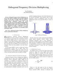
1. BASIC PRINCIPLES OF SPREAD SPECTRUM
Since 1940's spread spectrum systems were developed for antijam and low probability of
intercept (LPI) applications [10] by spreading the signal over a large frequency band and
transmitting it with a low power per unit bandwidth. In the antijam systems spectral
spreading secures the signal against narrowband interferers (Figure 1, [4]) and in the LPI
systems it to makes the detection as difficult as possible for an unwanted interceptor by
hiding the signal in the noise.
Figure 1 : Narrowband interference rejection ([4] : Figure 5.17)
In the spread spectrum systems instead of allocating disjoint frequency channels or time
slots for different users the simultaneous users are on the same frequency band. The
fundamental problem of spread spectrum in a multiple access communication application
(code division multiple access, CDMA) is that each user causes multiple access
interference (MAI) affecting all the other users. When the spectral efficiency of the
different multiple access methods was calculated by taking into account the original
signal bandwidth, the guard bands for FDMA, guard time for TDMA and MAI for
CDMA but not the channel properties the following results were obtained : (Table 1) [4].
3

Table 1 : Summary of multiple access technologies ([4] Dixon, Spread Systems with
Commercial Applications : Table 12.2 )
Lower level of spectral efficiency was obtained for CDMA. In the early multiple access
systems CDMA did not give clear advantage over TDMA/FDMA. The narrowband
methods FDMA and TDMA are more sensitive to channel impairments but unless they
are serious enough MAI is the dominating source of errors. Error probability calculations
based on MAI modeled as AWGN can be found in [2] and [3].
However, recently spread spectrum technology has become a viable alternative for
cellular systems. The advantages of using spread spectrum for cellular applications
include: inherent multipath diversity (large bandwidth allows using many multipath
components in the RAKE receiver), soft capacity (by exploiting the capacity without
reallocating channels), soft hand off capability, improved spectral efficiency (no need for
the frequency reuse distance between cells and guard bands of adjacent frequencies)
narrow band interference rejection (Figure 1, [4]) and inherent message privacy.[1] The
main disadvantage of spread spectrum is caused by MAI: the detected signals must be
controlled to have equal power to avoid the near-far effect.
In a spread spectrum system the data symbols x = {x n } are modulated onto a carrier by
using a spreading sequence (signature sequence, spreading code) a = {a k } that is different
for each user. This sequence spreads the transmitted signal bandwidth to be much larger
than the data signal bandwidth. The spread spectrum system contains the following
operations : data modulation of bits to symbols, spreading (bandwidth expansion) and
carrier modulation [5] :
4

Transmitter :
Receiver :
Spreading can be performed either on the baseband or on the carrier frequency:
Data
bits
Data
modulation
Data
symbol
sequence
x n
Spreading
Passband signal :
Re{a(t)⋅x(t)⋅e j2πft }
Despreading
Data
symbol
sequence
x n
Data
demodulation
Data
bits
Spreading
sequence a n
Spreading
sequence a n
Possible places for carrier modulation and demodulation
Figure 2
Because in general the data and spreading sequences are complex the transmitted signal
can be modeled as the real part of the product of three complex signals :
{ e j 2π f t c
a(
t)
⋅ x(
t)
}
s( t)
= Re ⋅
,where the part a(t)⋅x(t) that is used to modulate the carrier is called the complex envelope
The complexity is implemented by the phase-shifted I- and Q-carriers. (The signals with
real and imaginary parts are drawn by double lines in Figure 2).
5

When spreading is performed in time domain, i.e. the chips of the signature sequence are
placed in different chip periods T c the spread spectrum method is :
1. Direct sequence CDMA (DS-CDMA) when each symbol x n is spread into a sequence of
chips on a single carrier.
Thespreadingwaveforma(
t)
= A⋅
a
are used to modulatea singlecarrier f
, where
h ( t − kT ) and data waveform
x(
t)
= A⋅
x u
( t − nT)
withthebasebandcomplex
evelope s~ ( t)
= a(
t)
⋅ x(
t)
h ( t) and u(
t) are therealchipand bit amplitudeshapingfunctions
c
k
c
k
c
c
n
n
T
Data symbol
Sprading
sequence :
1 1-1 1-1 1-1
t
t
2. Frequency hopping CDMA (FH-CDMA) when each data symbol x n is spread into a
sequence of chips on different frequence shifts f k of the central carrier frequency f c . It is
modulated by the complex envelope
~ j f
k
t
s (
2π
t)
= x(
t)
⋅ h ( t − kT ) ⋅ e
Data symbol
k
c
c
t
Spreading
sequence :
f 1 f 2 f 3 f 4 f 4 f 5 f 6
1 1-1 1-1 1
t
3. Time hopping CDMA (TH-CDMA) when the chips a k are used to modulate a single carrier
by placing one chip inside the symbol frame T at a different time slot T c for each sequential
symbol.
Data symbols
t
Spreading
sequence :
t
When the spreading modulation is performed in the frequency domain the chips of the
signature sequence are used to modulate simultaneously different orthogonal subcarriers.
This spectrum method is called multicarrier CDMA (MC-CDMA). Instead of modulating
each sequential symbol on a different subcarrier (typically in OFDM) the same symbol x n
is in MC-CDMA used to modulate all the subcarriers f k = k⋅∆f by using a different chip
values a k for each subcarrier.
6

However, OFDM can be used together with MC-CDMA by converting a block of serial
data symbols into a block of parallel data symbols and modulating each parallel symbol
on a different set orthogonal subcarriers.
Data
sequence
x 1 …x N
Serial
Parallel
Converter
x 1
Spreading
modulator
x 1 a 1 e j2π∆ft
x 1 a K e j2πK∆ft
X 2
x N
Figure 3 [6]
1.1 DIRECT SEQUENCE (DS) SPREAD SPECTRUM
In a DS spread spectrum system (Data modulated carrier is modulated directly by a code
sequence) the ratio of the symbol and chip periods is called the processing gain G = T / T c
The temporal length of one code period of a short code sequence is equal to the symbol
period (G = N, T =N⋅T c ). The code period of a long code sequence contains several
symbol periods (G

Figure 4 : Complex spreading ([1] : Figure 9.2)
1.1.2 Dual channel quaternary spreading :
When the spreading sequence a(t) is real the I- and Q-channels have independent
spreading sequences a I (t) and a Q (t). The data sequence x(t) can be QPSK modulated or
consist of independent BPSK modulated data sequences x I (t) or x Q (t). When BPSK data
modulation is used x(t) is real and x I (t) and x Q (t)are independent data sequences
a(t)=a I (t) and a Q (t)
(real sequence)
x(t)= x I (t) +j⋅ x Q (t) or x(t)= x I (t) and x Q (t) (complex or 2 real sequences)
a I,Q = {a k : a k ∈{±1,}} , x I,Q ={x n :x n ∈{±1/√2,±j /√2},
This can be implemented by the dual channel quaternary spreading circuit :
Figure 5 : Dual channel quaternary spreading
([1] : Figure 9.3)
1.1.3 Balanced quaternary spreading :
When the spreading sequence is real a(t) having independent sequences a I (t) and a Q (t)
for the I- and Q-carrier and only one real BPSK data sequence x(t) is used
a(t)=a I (t) and a Q (t)
(real sequences)
x(t)
(one real data sequence)
a I,Q = {a k : a k ∈{±1,}} , x={x n :x n ∈{±1}
8

This can be implemented by the balanced quaternary spreading circuit :
Figure 6 :Balanced quaternary
spreading ([1] : Figure 9.4b)
1.1.4. Simple binary spreading :
One real BPSK modulated data sequence can be also spread to a single carrier by the
simple binary spreading :
a(t)
(one real spreading sequence)
x(t)
(one real data sequence)
a = {a k : a k ∈{±1,}} , x={x n :x n ∈{±1}:
Figure 7 : Simple binary spreading
([1] : Figure 9.4a)
The DS spread spectrum receiver performs the following functions: code synchronization
with the incoming sequence, phase synchronization with the incoming phase in the case
of coherent detection, despreading and filtering the signal and detecting the data. Code
and phase synchronization consist of acquisition and tracking operations.
The received signal can be despread by using a matched filter or correlator. Matched
filters are used with incoherent detection and for code acquisition with the coherent
detection.
9

Figure 8 : Simplified DS/QPSK system ([1] : Figure 9.1)
The bit error probability of DS/QPSK with Gray coding given by a ML receiver in an
AWGN channel is identical to QPSK [1]:
P
e
( 2⋅
E / N )
= Q
, which is identical to conventional coherent QPSK.
b
0
Spreading and despreading do not improve P e in an AWGN-channel because bandwidth
expansion is independent of data and spreading does not affect the spectral and
probability density functions of AWG-noise [1] ,[7].
DS spread spectrum system with pseudonoise sequencies is an averaging type system.
Multiple access interference from other users is reduced by averaging it.
1.2 FREQUENCY HOP (FH) SPREAD SPECTRUM
In frequency hopping spread spectrum systems the carrier frequency hops throughout a
finite set of frequencies during the code period. FH spread spectrum system is an
avoidance type system in which interference is reduced by avoiding same frequencies.
There are two basic types of FH spread spectrum: slow frequency hopping (SFH) and fast
frequency hopping (FFH). SFH systems transmit one or more data symbols per hop. FFH
systems transmit the same data symbol on multiple sequential hop frequencies.
10

Figure 9 : Simplified FH system operating on an AWGN channel ([1] : Figure 9.5)
When M-ary frequency shift keying (MFSK) is used as data modulation ∆f is the
frequency separation between symbols x k . The hopping frequencies f h are frequency
shifts relative to the center frequency determined by the symbol x k . The complex envelope
for slow frequency hopping is ([1]: (9.17)) :
~ L
jx π∆f
⋅t+
2 π f ⋅t
nL+
i
n
s ( t)
= A e
u ( t − ( nL + i)
T )
n i=
1
The complex envelope for fast frequency hopping is ([1]: (9.18)) :
~ L
jx π∆ f ⋅t+
2 π f
+
n
nL i
s ( t)
= A e
u ( t − ( nL + i)
T / L)
n i=
1
⋅t
T
T
The inner sum indexes for SFH the data symbols and for FFH the hopping frequencies.
The FH spread spectrum system may use coherent or incoherent detection but especially
for FFH the coherent frequency synthesizer is difficult to implement.
11

2. SPREADING SEQUENCES
The spreading sequences can be classified as orthogonal sequences and pseudonoise (PN)
sequences. The cross correlation of the orthogonal sequences is zero and so MAI from
other users is cancelled. Orthogonal sequences are used in synchronous CDMA systems
because the cross correlation function varies remarkably as a function of the time shift of
the sequences.
The pseudonoise (PN) sequences have auto-correlation function that is similar to white
Gaussian noise. The received sequences from other users are also noise-like signals. MAI
from other users is distributed evenly in time and between the interfering users. This
allows asynchronous operation. They are chosen to have three desirable attributes [1]:
1) Each element of the sequence (1,0 or +1,-1) occurs with equal frequency,
2) The auto-correlation has small off-peak values to allow rapid sequence acquisition and
3) Cross-correlation is small at all delays.
However, the attributes 2) and 3) are difficult to achieve simultaneously. Designing the
sequences to have low cross correlation reduces the randomness of the sequences and
increases the off-peak values of the auto-correlation function. [8]
Spreading sequences are often characterized in terms of their discrete-time correlation
properties with the time shift n. When short codes are used the auto- and cross-correlation
are calculated over a full sequence period N. When they are calculated periodically the
values of sequential data symbols are ignored.
The periodic auto-correlation of the k-th complex spreading sequence a (k) over a a full
period N is ([1])
φ
k,
k
1
( n)
=
2N
N −1
i=
0
a
*
( k ) ( k )
i ai+
n
and the periodic cross-correlation over a full period N between the k-th and m-th sequences
a (k) and a (m) is ([1])
φ
k,
m
1
( n)
=
2N
N −1
i=
0
a
( k )
i
a
( m)
i+
n
*
The aperiodic auto-correlation over the full period N of the sequence a (k) calculates only
the overlapping part of the sequences ([1]).
12

φ
a
k,
k
1
2N
1
( n)
=
2N
N −n
i=
1
N + n
i=
1
a
a
0
( k )
i+
n
( k )
i
a
a
( k )
i
( k )
i−n
*
*
, 0 ≤ n ≤ N −1
, − N + 1 ≤ n ≤ 0
, n ≥ N
Similar equations are obtained for the aperiodic cross-correlation of sequences a (k) and
a (m) over a full period N.
Periodic cross-correlation over full
period :
a k :
N=T
a m :
Aperiodic cross-correlation
over full period:
a k :
a m :
kT
(k+1)T
n>0
t
kT
(k+1)T
t
Figure 10 : Periodic and aperiodic full period auto- and cross-correlations
a
φk, k ( n)
= φ k,
k ( n)
+ φ k,
k ( n − N )
a
[] 2
By using the aperiodic auto-correlation the effect of different consequent symbols can be
taken into account [2]:
a
a
φ , ( n,
b−1,
b0
) = b0
⋅φ
k,
k ( n)
+ b−1
⋅φ
k,
k ( n − N ) , b−1
and b0
are consequent symbols ( + 1,-1)
k k
When long codes are used the partial period auto- and cross-correlations are calculated
over the bit period T=G⋅T c instead of the whole sequence period N ([1]).
φ
φ
p
k,
k
p
k,
m
1
( n)
=
2G
G −1
a
i = 0
1
( n)
=
2G
G−1
i=
0
*
( k ) ( k )
i ai
+ n
a
( k )
i
a
( m)
i+
n
*
13

Periodic correlation over
partial period:
a k :
a m :
Aperiodic correlation over
partial period:
a k :
a m :
kT
(k+1)T
t
Symbol period
t
Sequence period
Figure 11 : Periodic and aperiodic partial period auto- and cross-correlations
The partial period correlations are not only a function of the delay n, but also depend
upon the point in the sequence where the summation actually starts. They are difficult to
derive analytically. Therefore, statistical auto- and cross-correlations are used assuming
that the sequences with elements {±1,±j} are randomly generated.
The mean and variance of the partial period autocorrelation (periodic) are ([1])
G−
k m
[ k k n ] = E[ ai
ai
+ n ]
p 1 1
*
( ) ( )
φ , ( )
( n)
= E
= n,
2G
µ φ
δ
p
k , k
N
i=
0
2 p
2
2
1 0 . n = N
p
σ φ k , k ( n)
= E φ k,
k ( n)
− µ φ k k n = ( − n N ) =
p
, ( ) 1 δ ,
G 1/
G , n ≠ N
1.
n = N
=
0 , n ≠ N
The mean and variance of the partial period cross-correlation (periodic) are ([1])
[ φ
p k m(
n)
] = 0 , ∀n
µ φ m( n)
= E
p
,
2
p
2
n E
n
2
σ φ p
k , m ( ) = φ k,
m(
) − µ φ
p
k , m ( n)
= 1/ G , ∀n
14

2.1 SPREADING WAVEFORMS
In asynchronous systems the auto- and cross-correlation for the continuous-time waveforms
depend also on the amount of overlapping δ of the chip waveforms :
h c (t)
0
T c
c k
t'
c k
t'
δ
l
Figure 12 : Chip overlapping
The continuous-time periodic cross-correlation over a full period between the spreading
waveforms a (k) (t) and a (m) (t) depends both on the time shift between the sequences l
(earlier n) and the chip overlapping time shift δ ([1]) :
R
k,
m
1
T
( k)
( m)
( τ ) = a ( t)
a ( t + τ ) dt
T 0
= φ ( )
R ( δ ) + φ ( + 1) Rˆ
k,
m
h
k,
m
h
( δ )
For rectangular chip waveform h c (t) = u Tc (t) :
δ
Rk
, m( ) φk,
m(
) 1
− + φk,
m(
+ 1)
Tc
T
, τ = T
, R
h
c
( δ ) , Rˆ
+ δ
δ
τ , τ = T
+ δ
= c
c
h
( δ ) : chip waveformcorrelations
The maximum auto- and cross-correlations are obtained by the chip-synchronous
approximation (δ=0) :
Rk
, k ( τ ) ≤ φk,
k ( )
, Rk,
m(
τ ) ≤ φk,
m(
)
The partial period auto- and cross correlations are statistical funtions.
2.2 M-SEQUENCES
A widely used type of PN sequences are the maximum-length shift-register sequences
(LFSR), m-sequences. Each sequence is generated by a separate LFSR that has m stages.
The period of the sequence (sequence length) is N = 2 m –1. They are the longest
sequences that can be generated by an LFSR for a given m. [1]
15

Figure 13 : m-sequence generator ([1] : Figure 9.6)
The multipliers p i ∈ {0,1} and ⊕ denotes modulo 2 addition . The elements (chips) of
the sequence a i ∈ {0,1} are mapped to {+1,-1} for bipolar coding. The sequence a(k) has
2 m-1 ones and 2 m-1 –1 zeros.
The feedback polynomial is a primitive polynomial of degree m over GF(2) [1] :
P(x) = 1 ⊕ p 1 x ⊕ p 2 x 2 ⊕ p 3 x 3 ⊕ … ⊕ p m-1 x m-1 ⊕ x m
An m-sequence has almost an ideal full period autocorrelation :
1
, n = N
φ( n)
=
−1/
N , n ≠ N
The full period auto-correlation function for continuous time sequence waveforms a (k) (t)
when the rectangular chip shaping function h c (t) = u Tc (t) is used is :
R
δ
δ
τ ) = φk,
k ( ) 1
− + φk
k ( + 1) , τ = Tc
+ δ
Tc
Tc
k,
k ( ,
Figure 14 : Typical full period autocorrelation function of
an m-sequence spreading waveform ([1] : Figure 9.7)
16

However, only for certain values of m there exist some pairs of m-sequences with low full
period cross-correlation. When the average full period cross-correlation between
sequences a (k) and a (m) is calculated for different shifts n of the sequences:
θ =
N
1 N −1
φ
n=
0
( )
k, m n
the value of θ varies much depending on the particular pair of m-sequences that are
selected and the worst θ-values are great.
Tabel 2 : Best and worst case average cross-correlations for m-sequences
([1]: Table 9.1)
Figure 15 : Cross-correlation function of typical m-
sequences ([4])
17

2.3 GOLD SEQUENCES
A set Gold sequences consist of 2 m+1 sequences having the period N = 2 m –1 that are
generated by a preferred pair of m-sequences. This set contains both the preferred pair
(a (1) ,a (2) ) and the 2 m -1 new generated sequences. The sequences are generated by taking a
modulo-2 sum of a (1) with the 2 m-1 cyclically shifted versions of a (2) or vice versa.
Figure 16 : A Gold sequence generator with p 1 (x)= 1+x 2 +x 5 and p 2 (x)= 1+x+x 2 +x 4 +x 5
This sequence generator can produce 32 Gold sequences of length 31. ([1]: Figure 9.8)
Because the Gold sequences are not maximal length sequences (except a (1) and a (2) ) the
auto-correlation function is not 2-valued. Both the cross-correlation and off-peak autocorrelation
functions are 3-valued : {-1, -t(m), t(m)-2}, where
2
t(
m)
= (
2
( m+
1) / 2+
1
m+
2) / 2
+ 1
, when
, when
m is odd
m is even
So both the cross correlation and off-peak auto-correlation functions are upper bounded
by t(m) :
18

Table 3 : Peak cross correlation of m-sequences and Gold-sequences
([1] : Table 9.2)
2.4 KASAMI SEQUENCES
The small set of Kasami sequences consists 2 m/2 sequences having the period N = 2 m –1.
This set is generated in a way similar to the Gold sequences by using a pair of a long
sequence a (1) and a short sequence a (2) that are m-sequences. This set contains both the
long sequence a (1) and the 2 m/2 -1 new generated sequences. The sequences are generated
by taking a modulo-2 sum of a (1) with all the 2 m/2 -1 cyclic shifts of a (2) .
Figure 17 : A Kasami sequence generator with p 1 (x)= 1+x+x 6 and
p 2 (x)= 1+x+x 3 . This sequence generator can produce 8 Kasami
sequences of length 63. ([1]: Figure 9.9)
19

Like for Gold sequences the cross-correlation and off-peak auto-correlation functions are
3-valued. The possible values are : {-1, -s (m), s(m)-2}, where
/ 2
t(
m)
= 2
m + 1
The upper bound s(m) for the cross correlation and off-peak auto-correlation functions is
reduced to half compared with the Gold sequences of the same length.
The large set of Kasami sequences contains also Gold sequences and hence the crosscorrelation
and off-peak autocorrelation values are on the average higher than in the small
set of Kasami sequences.
2.5 BARKER SEQUENCES
The Barker sequences are aperiodic sequences (finite length sequences). Their crosscorrelation
and off-peak auto-correlation values are limited by 1/N but they are known
only for code lengths N=2,3,4,5,7,11. Because the Barker sequences are short and their
number is limited they are used for special purpose systems (as for initial synchronization
and wireless LANs). 1
,n = 0
φ
a
k
, k
( n)
=
0,
1
N
1
or −
N
,n ≠ 0
2.6 WALSH-HADAMARD SEQUENCES
The Walsh-Hadamard sequences are orthogonal sequences. They are the rows of the
Hadamard matrix that is obtained by the recursion :
H
M H M
1
1
H 2 M =
starting from H 2 =
H
M − H
M
1
−1
The Walsh-Hadamard sequences can be used either to spread orthogonally (orthogonal
CDMA) the signals of the different users or for M-ary orthogonal coding the different
symbols.
If orthogonal sequences are used for different users accurate synchronization is needed
because the orthogonal sequences have for non-zero time shifts large cross-correlation
and off-peak auto-correlation values.
If orthogonal symbols are used k=log 2 M bits are used to encode one of the orthogonal
symbols. The user signals are spread by different pseudonoise sequences.
20

3. POWER SPECTRAL DENSITY OF DS SPREAD SPECTRUM
SIGNALS
For uncorrelated zero-mean data symbols the power spectral density of the baseband
complex envelope is ([1] : 4.206)
2
A 2
S~ s~
s ( f ) = σ x H a ( f )
T
2
([]
1 : 9.58)
,where h a (t) is the amplitude shaping waveform determined by the spreading sequence a k
and the chip pulse waveform h c (t)
h ( t)
a
H
a
N 1
=
− ak
c
k = 0
2
c
h ( t − kT )
c
([]
1 : 9.59)
2
( f ) = H ( f ) ⋅ N ⋅Φ
( f )
([]
1 : 9.62)
2 k,
k
,where Φ k,k (f) is the discrete Fourier transform of the aperiodic autocorrelation function
φ k,k (n) of the spreading sequence a k .
The power spectral density depends on the spectral product of the chip pulse waveform
h c (t) and spreading sequence a k :
2
A 2 2
S~ s~
s ( f ) = σx
Hc(
f ) ⋅Φk,
k(f
)
T
c
([]
1 : 9.64)
For example for the rectangular chip pulse waveform h c (t) and ideal aperiodic autocorrelation
function:
a
φ k
S
1
, k ( n)
=
0
2
( f ) = A T
, n = 0
, n ≠ 0
2
~ s ~ s
c ⋅sinc
(fTc
)
The effect of the deviation from the ideal aperiodic auto-correlation function is calculated
for the length-11 Barker sequence :
a (1) = (-1 +1 –1 –1 +1 –1 –1 –1 –1 +1 +1 +1) and
for the length-15 m-sequence :
a (2) = (+1 -1 –1 +1 -1 –1 –1 + 1 + 1 +1 +1 –1 +1 –1 +1)
Because the 11-Barker sequence has the aperiodic auto-correlation function that is closer
to the ideal one it has smoother power spectral density. For this reason the length-11
Barker sequence has been chosen for the IEEE 802.11 wireless LAN specification.
21

Figure 18 ([1]: Figure 9.11) Aperiodic
autocorrelation function for the length-11
Barker sequence
Figure 19 ([1]: Figure 9.12) Aperiodic
autocorrelation function for the length-15
m-sequence
Figure 20 ([1]: Figure 9.13) PSD with the
length-11 Barker sequence
Figure 21 ([1]: Figure 9.14) PSD with the
length-11 Barker sequence
22

REFERENCES
[1] Gordon L. Stuber :
Principles of mobile communication, 2 nd edition, 2001,
Kluwer Academic Publishers
[2] Michael B. Pursley :
Performance Evaluation for Phase-Coded Spread-Spectrum
Multiple-Access Communication
– Part I : System Analysis.
Michael B. Pursley, Philip V. Sarwate:
– Part II : Code Sequence Analysis
IEEE Transactions on Communications, Vol.Com-25, No. 8, August 1977
[3] Michael B. Pursley, Philip V. Sarwate, Wayne E. Stark :
Error Probability for Direct-Sequence Spread-Spectrum Multiple-Access Communications
– Part I: Error Probability for Direct-Sequence Spread-Spectrum Multiple-Access
Communications :Upper and Lower Bounds,
Evaggelos A. Geraniotis, Michael B. Pursley :
– Part II: Approximations,
IEEE Transactions on Communications, Vol.Com.-30, No. 5, 11, May 1982
[4] Robert C. Dixon :
Spread Spectrum Systems with Commercial Applications, 3 nd edition, 1994,
John Wiley & Sons
[5] Robert A. Scholtz :
The Spread Spectrum Concept,
IEEE Transactions on Communications, Vol.Com-25, No. 8, August 1977
[6] Ramjee Prasad :
Personal Mobile Communications, 1995,
McGraw-Hill Series in Electrical Engineering
[7] Kamilo Feher : Wireless Digital Communications, Prentice Hall ,1995, pp. 285-332
[8] Tero Ojanperä, Ramjee Prasad : Wideband CDMA for Third Generation
Mobile Communications
Artech House, 1998
[9] Stefan Parkvall :
Variability of User Performance in Cellular DS-CDMA –
Long versus Short Spreading Sequences
IEEE Transactions on Communications, Vol. 48, No. 7, July 2000
[10] Robert A. Scholtz :
The Origins of Spread-Spectrum Communications,
IEEE Transactions on Communications, Vol.Com.-30, No. 5, May 1982
23