SEA Modelling for Sound Package Development Inclusion ... - Rieter
SEA Modelling for Sound Package Development Inclusion ... - Rieter
SEA Modelling for Sound Package Development Inclusion ... - Rieter

You also want an ePaper? Increase the reach of your titles
YUMPU automatically turns print PDFs into web optimized ePapers that Google loves.
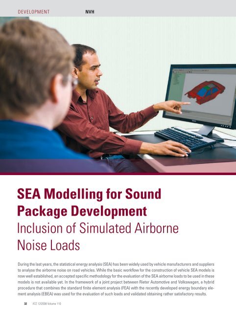
<strong>Development</strong><br />
NVH<br />
<strong>SEA</strong> <strong>Modelling</strong> <strong>for</strong> <strong>Sound</strong><br />
<strong>Package</strong> <strong>Development</strong><br />
<strong>Inclusion</strong> of Simulated Airborne<br />
Noise Loads<br />
During the last years, the statistical energy analysis (<strong>SEA</strong>) has been widely used by vehicle manufacturers and suppliers<br />
to analyse the airborne noise on road vehicles. While the basic workflow <strong>for</strong> the construction of vehicle <strong>SEA</strong> models is<br />
now well established, an accepted specific methodology <strong>for</strong> the evaluation of the <strong>SEA</strong> airborne loads to be used in these<br />
models is not available yet. In the framework of a joint project between <strong>Rieter</strong> Automotive and Volkswagen, a hybrid<br />
procedure that combines the standard finite element analysis (FEA) with the recently developed energy boundary element<br />
analysis (EBEA) was used <strong>for</strong> the evaluation of such loads and validated obtaining rather satisfactory results.<br />
32<br />
ATZ 12I2008 Volume 110
The Authors<br />
1 Introduction<br />
When a test vehicle is available, the experimental<br />
evaluation of the sound pressure<br />
level distribution around the vehicle<br />
of interest represents a robust and<br />
sensible approach <strong>for</strong> the definition of<br />
the airborne loads to be used in its statistical<br />
energy analysis (<strong>SEA</strong>) model. This<br />
approach has been used by many <strong>SEA</strong><br />
analysts with satisfactory results, and in<br />
a first attempt, it was used also <strong>for</strong> the<br />
joint <strong>Rieter</strong>/Volkswagen <strong>SEA</strong> simulation<br />
project, in cooperation with University<br />
Michigan (USA) considered here. Papers<br />
[1] to [3] represent just a very small selection<br />
of the dozens of papers that have<br />
been published on this topic during the<br />
last 15 years.<br />
For the evaluation of the airborne<br />
loads, the outer panels of the vehicle<br />
passenger compartment are subdivided<br />
in a way compatible with the subdivision<br />
of the <strong>SEA</strong> model into subsystems.<br />
After this, <strong>for</strong> each panel, a few measurement<br />
positions close to the panel<br />
surface are defined. The total number of<br />
measurement positions can range from<br />
200 to 350, depending on the vehicle’s<br />
size. The sound pressure level generated<br />
by one or more sound sources at each<br />
one of these positions is evaluated. The<br />
joint activity between <strong>Rieter</strong> and Volkswagen<br />
focused on the acoustic transfer<br />
function from the rear tyre as noise<br />
source and, <strong>for</strong> this case, Volkswagen<br />
test standards prescribe considering<br />
eight different source positions, four<br />
around each rear tyre. For each panel,<br />
the airborne load to be applied in the<br />
<strong>SEA</strong> model is obtained by energetically<br />
averaging both on the microphone positions<br />
lying on the panel itself and on all<br />
source positions.<br />
As already mentioned, this whole<br />
process has proven to be reliable and robust.<br />
But in some cases it might represent<br />
a weak point in the construction<br />
process of the <strong>SEA</strong> model:<br />
– The necessary testing is timely quite<br />
extensive: depending on the number<br />
of source positions to be analysed and<br />
on the hardware available, it can take<br />
from one to three weeks.<br />
– If the <strong>SEA</strong> model is intended to assist<br />
the development of a vehicle sound<br />
package, the measurement of the <strong>SEA</strong><br />
loads assumes the availability of a vehicle<br />
prototype.<br />
– Even when the vehicle is available,<br />
the measured <strong>SEA</strong> loads are introduced<br />
into the <strong>SEA</strong> model as “static<br />
constraints”. This precludes the ability<br />
to simulate the effect of design<br />
changes related to the external shape<br />
of the vehicle, the position of the<br />
source and the presence and the positioning<br />
of absorbing materials.<br />
As a consequence of all this, <strong>SEA</strong> analysts<br />
have long tried to develop techniques<br />
that allow at least to estimate the <strong>SEA</strong><br />
airborne loads without the need of experimental<br />
tests. In most cases, semi-empirical<br />
procedures based mainly on „trial-and-error“<br />
were used and, <strong>for</strong> many<br />
years, these techniques have remained at<br />
the level of „confidential recipes”. Only<br />
relatively recently have some specific<br />
Dipl.-Phys.<br />
Boris Brähler<br />
is technical expert <strong>for</strong><br />
acoustics in the Centre<br />
of Excellence <strong>for</strong> Vehicle<br />
Acoustics at <strong>Rieter</strong><br />
Automotive in Winterthur<br />
(Switzerland).<br />
Dipl.-Phys.<br />
Claudio Bertolini<br />
is responsible <strong>for</strong> NVH<br />
tools and methodologies<br />
in the Centre of<br />
Excellence <strong>for</strong> Vehicle<br />
Acoustics at <strong>Rieter</strong><br />
Automotive in Winterthur<br />
(Switzerland).<br />
Figure 1: Schematic representation of the radiation from a vibrating body in a half-space<br />
(with reflexion panel S H<br />
)<br />
ATZ 12I2008 Volume 110 33
<strong>Development</strong><br />
NVH<br />
works on this topic been published [4, 5].<br />
In particular, a very promising methodology<br />
<strong>for</strong> the efficient analysis of radiation<br />
and scattering problems in the midhigh<br />
frequency range was proposed by<br />
Wang, Vlahopoulos and Wu [6]. This<br />
methodology was called energy boundary<br />
element analysis (EBEA) by the authors<br />
since it essentially consists of an energetic<br />
re<strong>for</strong>mulation of the classical integral<br />
equations on which the boundary<br />
element analysis (BEA) is based.<br />
Figure 2: Model used <strong>for</strong> EBEA simulations; the source positions around the rear left tyre are<br />
visible, as well as some response positions around the vehicle’s part panels<br />
2 Brief Review of Energy<br />
Boundary Element Analysis<br />
EBEA equations are essentially an energetic<br />
re<strong>for</strong>mulation of classical BEA equations.<br />
Given a vibrating body delimited by<br />
a boundary surface S in presence of a rigid<br />
halfplane S H<br />
, Figure 1, classical BEA integral<br />
equations allow to express the acoustic<br />
pressure at a receiver point M as Eq. (1):<br />
pˆ(M) = ∫ S<br />
A(P)G(P, M)dS Eq. (1)<br />
where P is a generic point located on the<br />
surface S, A(P) is an unknown complex<br />
source strength defined on S, and Eq. (2)<br />
___<br />
g(P, M) = e–ikr<br />
4πr<br />
____<br />
4πr<br />
Eq. (2)<br />
1<br />
+ e–ikr1<br />
is the half-space Green’s function (see<br />
Figure 1 <strong>for</strong> the explanation of the notations<br />
used in Eq. (2)). Starting from Eq. (1)<br />
and under the basic assumption that the<br />
spatial correlation between the average<br />
acoustic fields in different regions<br />
around the vibrating body is zero, it is<br />
possible to express the average acoustic<br />
energy density and the average acoustic<br />
intensity at M as Eq. (3) and Eq. (4):<br />
E[‹ › e ] =<br />
Eq. (3)<br />
_____ ρ _____<br />
∫ S<br />
σ ( <br />
64π 2 r<br />
+ k2 ρ ______ ρ ______<br />
4 32π 2 r<br />
+ 2 64π 2 4<br />
r<br />
+ k2 ρ<br />
1<br />
32π 2 2<br />
r<br />
)dS<br />
1<br />
E[‹ I › ] = ∫ S σ ( k2 ρc _____<br />
where<br />
______<br />
32π 2 r<br />
E 2 r<br />
+ k2 ρc<br />
32π 2 2<br />
r<br />
E r1 1<br />
)dS Eq. (4)<br />
σ = ____ 1<br />
ρ 2 ω<br />
|A| 2 Eq. (5)<br />
2<br />
is defined as the strength density of the<br />
energy source and it is a frequency dependent<br />
quantity directly linked to A. In<br />
Eq. (3) and Eq. (4), E[ ] indicates frequency<br />
or space averaging. Comparing to the<br />
conventional BEA integral Eq. (1) <strong>for</strong> halfspace<br />
problems to Eq. (3) and Eq. (4), it<br />
turns out that, in a <strong>for</strong>mal way, EBEA is<br />
similar to BEA in the sense that it makes<br />
use of surface integral equations <strong>for</strong> the<br />
evaluation of the primary quantities of<br />
interest. In the case of EBEA, differently<br />
from BEA, such quantities are of an energetic<br />
nature, being given by the acoustic<br />
energy density and intensity. The halfspace<br />
Green’s functions <strong>for</strong> the acoustic<br />
energy density and intensity are given by<br />
Eq. (6) and Eq. (7):<br />
_____ ρ _____<br />
G = <br />
64π 2 r<br />
+ k2 ρ ______ ρ ______ k 4 32π 2 r<br />
+ 2 64π 2 4<br />
r<br />
+ <br />
2 ρ<br />
1<br />
32π 2 2<br />
r<br />
Eq. (6)<br />
1<br />
_____<br />
H = k2 ρc ______<br />
32π 2 r<br />
E 2 r<br />
+ k2 ρc<br />
32π 2 2<br />
r<br />
E r1<br />
Eq. (7)<br />
1<br />
In order to develop a numerical solution,<br />
the surface S of the model is divided into<br />
n quadrilateral or triangular elements.<br />
The source strength density σ j<br />
on each<br />
element is assumed to be a constant. Eq.<br />
(3) and Eq. (4) are rewritten in a discrete<br />
<strong>for</strong>m as Eq. (8) and Eq. (9):<br />
E[‹ › e ] = Y [<br />
j=1 Σn σ j<br />
∫ Sj<br />
G(ξ, Y)dS ] Eq. (8)<br />
E[‹ › I ] = Y [<br />
j=1 Σn σ j<br />
∫ Sj<br />
H(ξ, Y)dS ] Eq. (9)<br />
Here, n is the number of the elements<br />
over the surface S, ξ is an arbitrary point<br />
on the element j, Y indicates the location<br />
of an arbitrary field point exterior to the<br />
structure in the half space. The outward<br />
radiated acoustic power on each element<br />
constitutes the boundary conditions of<br />
the EBEA <strong>for</strong>mulation, which is described<br />
as Eq. (10):<br />
∫ Si ‹ › I · n dS = P– , i = 1, 2, …, n Eq. (10)<br />
i i<br />
Substituting Eq. (10) in Eq. (9) results in<br />
Eq. (11):<br />
K ij<br />
σ j<br />
= P – ,<br />
i<br />
i = 1, 2, …, n, j = 1, 2, …, n<br />
Eq. (11)<br />
Eq. (11) is solved numerically. Then by<br />
employing Eq. (3) and Eq. (4), the acoustic<br />
energy density and intensity are determined<br />
at any field point in the half space<br />
exterior to the BEA model.<br />
3 Description of Hybrid FEA/EBEA<br />
Methodology <strong>for</strong> the Evaluation of<br />
<strong>SEA</strong> Loads<br />
In the application described in this article,<br />
a combination of standard FEA (<strong>for</strong><br />
the mid-low frequency range) and EBEA<br />
(<strong>for</strong> the high-frequency range) is used to<br />
evaluate the input value of airborne<br />
loads <strong>for</strong> a <strong>SEA</strong> model. The use of a deterministic<br />
FEA simulation methodology<br />
<strong>for</strong> the mid-low frequency range is related<br />
to the fact that EBEA is intrinsically<br />
well suited <strong>for</strong> the high-frequency range.<br />
When working on a discretised surface<br />
model, the methodology basically assumes<br />
that the (average) acoustic fields<br />
on different surface elements that constitute<br />
the model are uncorrelated. It is<br />
intuitive that this assumption tends to<br />
be more and more satisfied as the frequency<br />
increases and, correspondingly,<br />
the wavelength becomes smaller.<br />
Among the various possibilities, <strong>for</strong><br />
the calculations in the mid-low frequency<br />
range standard FE were preferred over<br />
BEA and infinite elements because of<br />
their higher computational efficiency<br />
34<br />
ATZ 12I2008 Volume 110
small spheres. Furthermore, also some<br />
of the response points used <strong>for</strong> the evaluation<br />
of the exterior sound pressure<br />
level are also marked. Since the computational<br />
ef<strong>for</strong>t <strong>for</strong> EBEA calculations is<br />
rather small, the model was run also in<br />
the mid-low frequency range. The set of<br />
response frequencies <strong>for</strong> the EBEA consisted<br />
of the 1/3 octave centre frequency<br />
bands, starting from 400 up to 8000 Hz.<br />
The computational time <strong>for</strong> the entire<br />
frequency range is approximately 10<br />
min <strong>for</strong> each source position, on a usual<br />
desk-top PC.<br />
Figure 3: <strong>Sound</strong> pressure level on the rear left door window panel (spatial and source<br />
average); comparison between measured and FEA/EBEA simulated data<br />
4 Validation Results<br />
and easiness in the preparation of the<br />
model. For the FE model, the acoustic<br />
space around the vehicle was meshed<br />
with four-node tetrahedral elements, up<br />
to a distance of about 0.65 m (that is<br />
about one wavelength at 500 Hz) from<br />
the vehicle external surfaces (roof, side,<br />
front and back). On the outer boundary<br />
of the FE box so obtained, a boundary impedance<br />
equal to the characteristic impedance<br />
of air was imposed. It is clear<br />
that this boundary condition is able to<br />
represent only approximately the infinite<br />
acoustic space around the vehicle, in particular<br />
at low frequency. Nevertheless, it<br />
has to be emphasised that the primary<br />
interest here lies in the evaluation of the<br />
sound pressure level at points that are<br />
very close to the vehicle surface and these<br />
points are not likely to feel strongly the<br />
details of the boundary conditions imposed<br />
on the outer surfaces of the model.<br />
A mesh size of 25 mm was chosen, resulting<br />
in an upper frequency limit of about<br />
2200 Hz <strong>for</strong> the validity of the model results.<br />
Overall, the resulting model is<br />
huge: it includes about 600,000 nodes<br />
and about 2.7 millions of elements.<br />
For each one of the panels of interest<br />
around the vehicle, a set of response<br />
nodes was defined. On average, about 25<br />
points per panel were taken. For each of<br />
the eight prescribed positions around<br />
the rear tyres, a unit volume velocity<br />
source was defined. Calculations were<br />
run from 300 up to 2500 Hz, with a frequency<br />
step of 25 Hz (this guarantees at<br />
least five response frequencies <strong>for</strong> each<br />
third octave band above 500 Hz). All calculations<br />
were run using MSC/Nastran<br />
on an HP-Itanium machine having 4 GB<br />
RAM and a 1.5 GHz processor. The total<br />
computational ef<strong>for</strong>t is quite remarkable:<br />
the solution of the model takes<br />
about 45 min per frequency and the total<br />
calculation time is about 65 h.<br />
Figure 2 shows the EBEA model used<br />
<strong>for</strong> the evaluation of the airborne loads<br />
<strong>for</strong> the <strong>SEA</strong> Model of the analysed<br />
Volkswagen vehicle. The model includes<br />
2245 nodes and 2436 elements, the average<br />
mesh size being about 150 mm. In<br />
Figure 2, some of the sources around the<br />
rear left tyre are visible, modelled as<br />
Figure 3 reports the measured sound pressure<br />
level on the rear left window, together<br />
with the simulation results obtained<br />
both with FEA and with EBEA. To<br />
allow a better understanding of the data,<br />
FEA results are plotted in narrow-band.<br />
As one can see, in the mid-low frequency<br />
range, FEA results are able to catch the<br />
general trend of the test data and also<br />
the corresponding absolute level. The<br />
same is true <strong>for</strong> the EBEA results, but<br />
only above 2 kHz. The frequency region<br />
around 2 kHz looks ideal <strong>for</strong> a merging<br />
of the FEA and the EBEA results: this is<br />
why, <strong>for</strong> the calculation of the <strong>SEA</strong> airborne<br />
loads, the FEA results were used,<br />
after converting them into third-octave<br />
bands, up to the 2 kHz frequency band<br />
Figure 4: Rear tyre acoustic transfer function <strong>for</strong> the rear left passenger’s head cavity;<br />
comparison between measurements, <strong>SEA</strong> results obtained with experimental airborne loads<br />
and <strong>SEA</strong> results obtained with simulated airborne loads<br />
ATZ 12I2008 Volume 110 35
<strong>Development</strong><br />
NVH<br />
included. Starting from the 2.5 kHz<br />
band, EBEA results were used.<br />
For most panels around the rear part<br />
of the vehicle, this allowed obtaining discrepancies<br />
lower than 3 dB between the<br />
measured and the simulated loads in<br />
third-octave bands. The <strong>SEA</strong> airborne<br />
loads obtained from the FEA/EBEA simulations<br />
were input into the <strong>SEA</strong> model of<br />
the Volkswagen vehicle under study and<br />
the results were compared with the ones<br />
obtained using the measured airborne<br />
<strong>SEA</strong> loads. Such comparison is reported<br />
in Figure 4 <strong>for</strong> the rear passenger’s head<br />
cavity, which is the cavity of main interest<br />
here. As one can see from this figure,<br />
the discrepancies between the <strong>SEA</strong> results<br />
obtained with the measured airborne<br />
loads and the <strong>SEA</strong> results obtained<br />
with the simulated airborne loads are<br />
more than acceptable, being generally<br />
lower than 1.5 dB.<br />
5 Conclusions<br />
References<br />
[1] Powell, R.; Zhu, J.; Manning, J. E.: <strong>SEA</strong> Modeling<br />
and Testing <strong>for</strong> Airborne Transmission Through<br />
Vehicle <strong>Sound</strong> <strong>Package</strong>. SAE Paper 971973, USA,<br />
1997<br />
[2] Parrett, A.; Hicks, J. K.; Burton, T. E.; Hermans, L.:<br />
Statistical Energy Analysis of Airborne and Structure-Borne<br />
Automobile Interior Noise. SAE Paper<br />
971970, USA, 1997<br />
[3] Bertolini, C.; Gigante, L.: An <strong>SEA</strong>-Based Procedure<br />
<strong>for</strong> the Definition of <strong>Sound</strong> <strong>Package</strong> Component<br />
Targets Starting From Global Vehicle Targets.<br />
VibroAcoustics Users’ Conference Europe, Leuven,<br />
Belgium, 2003<br />
[4] Blanchet, D.; DeJong, R.; Fukui, K.: <strong>Development</strong> of<br />
a Modeling Technique <strong>for</strong> Vehicle External <strong>Sound</strong><br />
Field Using <strong>SEA</strong>. Proceedings of Internoise 2004,<br />
Prag, Czech, 2004<br />
[5] Venor, J.; Burghardt, M.: <strong>SEA</strong> Modeling and<br />
Validation of <strong>Sound</strong>-Fields and Seals in Automobiles.<br />
Proceedings of EuroPam Conference 2005,<br />
Potsdam, Germany, 2005<br />
[6] Wang, A.; Vlahopoulos, N.; Wu, K.: <strong>Development</strong><br />
of an Energy Boundary Element Formulation <strong>for</strong><br />
Computing High-Frequency <strong>Sound</strong> Radiation From<br />
Incoherent Intensity Boundary Conditions. Journal<br />
of <strong>Sound</strong> and Vibration, Vol. 278, pp 413-436,<br />
Elsevier, Amsterdam, Netherlands, 2004<br />
The combination of standard FEA calculations<br />
with special EBEA (energy boundary<br />
element analysis) calculations allowed<br />
<strong>Rieter</strong> Automotive and Volkswagen<br />
to estimate the airborne statistical energy<br />
analysis (<strong>SEA</strong>) loads with an acceptable<br />
accuracy. The results of the <strong>SEA</strong> model<br />
obtained with the introduction of the<br />
simulated airborne loads compare rather<br />
well with those obtained with the experimental<br />
loads.<br />
The employment of such a model to<br />
support the acoustic vehicle development<br />
process is meaningful as there<strong>for</strong>e<br />
to judge. Some discrepancies are observed<br />
but these discrepancies remain within<br />
the limits that make it possible to use<br />
the model <strong>for</strong> design decisions. The proposed<br />
procedure still has a weak point in<br />
the computational ef<strong>for</strong>t needed <strong>for</strong> the<br />
FE calculations in the mid-low frequency<br />
range. Some further work would be advisable<br />
to develop numerical and experimental<br />
procedures that allow extending<br />
the use of EBEA as far as possible into the<br />
mid-low frequency range.<br />
36<br />
ATZ 12I2008 Volume 110