MECHANICS of FLUIDS LABORATORY - Mechanical Engineering
MECHANICS of FLUIDS LABORATORY - Mechanical Engineering
MECHANICS of FLUIDS LABORATORY - Mechanical Engineering

You also want an ePaper? Increase the reach of your titles
YUMPU automatically turns print PDFs into web optimized ePapers that Google loves.
A Manual for the<br />
<strong>MECHANICS</strong> <strong>of</strong> <strong>FLUIDS</strong> <strong>LABORATORY</strong><br />
William S. Janna<br />
Department <strong>of</strong> <strong>Mechanical</strong> <strong>Engineering</strong><br />
Memphis State University
©1997 William S. Janna<br />
All Rights Reserved.<br />
No part <strong>of</strong> this manual may be reproduced, stored in a retrieval<br />
system, or transcribed in any form or by any means—electronic, magnetic,<br />
mechanical, photocopying, recording, or otherwise—<br />
without the prior written consent <strong>of</strong> William S. Janna<br />
2
TABLE OF CONTENTS<br />
Item<br />
Page<br />
Report Writing.................................................................................................................4<br />
Cleanliness and Safety ....................................................................................................6<br />
Experiment 1 Density and Surface Tension.....................................................7<br />
Experiment 2 Viscosity.........................................................................................9<br />
Experiment 3 Center <strong>of</strong> Pressure on a Submerged Plane Surface.............10<br />
Experiment 4 Measurement <strong>of</strong> Differential Pressure..................................12<br />
Experiment 5 Impact <strong>of</strong> a Jet <strong>of</strong> Water ............................................................14<br />
Experiment 6 Critical Reynolds Number in Pipe Flow...............................16<br />
Experiment 7 Fluid Meters................................................................................18<br />
Experiment 8 Pipe Flow .....................................................................................22<br />
Experiment 9 Pressure Distribution About a Circular Cylinder................24<br />
Experiment 10 Drag Force Determination .......................................................27<br />
Experiment 11 Analysis <strong>of</strong> an Airfoil................................................................28<br />
Experiment 12 Open Channel Flow—Sluice Gate .........................................30<br />
Experiment 13 Open Channel Flow Over a Weir ..........................................32<br />
Experiment 14 Open Channel Flow—Hydraulic Jump ................................34<br />
Experiment 15 Open Channel Flow Over a Hump........................................36<br />
Experiment 16 Measurement <strong>of</strong> Velocity and Calibration <strong>of</strong><br />
a Meter for Compressible Flow.............................39<br />
Experiment 17 Measurement <strong>of</strong> Fan Horsepower .........................................44<br />
Experiment 18 Measurement <strong>of</strong> Pump Performance....................................46<br />
Appendix .........................................................................................................................50<br />
3
REPORT WRITING<br />
All reports in the Fluid Mechanics<br />
Laboratory require a formal laboratory report<br />
unless specified otherwise. The report should be<br />
written in such a way that anyone can duplicate<br />
the performed experiment and find the same<br />
results as the originator. The reports should be<br />
simple and clearly written. Reports are due one<br />
week after the experiment was performed, unless<br />
specified otherwise.<br />
The report should communicate several ideas<br />
to the reader. First the report should be neatly<br />
done. The experimenter is in effect trying to<br />
convince the reader that the experiment was<br />
performed in a straightforward manner with<br />
great care and with full attention to detail. A<br />
poorly written report might instead lead the<br />
reader to think that just as little care went into<br />
performing the experiment. Second, the report<br />
should be well organized. The reader should be<br />
able to easily follow each step discussed in the<br />
text. Third, the report should contain accurate<br />
results. This will require checking and rechecking<br />
the calculations until accuracy can be guaranteed.<br />
Fourth, the report should be free <strong>of</strong> spelling and<br />
grammatical errors. The following format, shown<br />
in Figure R.1, is to be used for formal Laboratory<br />
Reports:<br />
Title Page–The title page should show the title<br />
and number <strong>of</strong> the experiment, the date the<br />
experiment was performed, experimenter's<br />
name and experimenter's partners' names.<br />
Table <strong>of</strong> Contents –Each page <strong>of</strong> the report must<br />
be numbered for this section.<br />
Object –The object is a clear concise statement<br />
explaining the purpose <strong>of</strong> the experiment.<br />
This is one <strong>of</strong> the most important parts <strong>of</strong> the<br />
laboratory report because everything<br />
included in the report must somehow relate to<br />
the stated object. The object can be as short as<br />
one sentence and it is usually written in the<br />
past tense.<br />
Theory –The theory section should contain a<br />
complete analytical development <strong>of</strong> all<br />
important equations pertinent to the<br />
experiment, and how these equations are used<br />
in the reduction <strong>of</strong> data. The theory section<br />
should be written textbook-style.<br />
Procedure – The procedure section should contain<br />
a schematic drawing <strong>of</strong> the experimental<br />
setup including all equipment used in a parts<br />
list with manufacturer serial numbers, if any.<br />
Show the function <strong>of</strong> each part when<br />
necessary for clarity. Outline exactly step-<br />
Bibliography<br />
Calibration Curves<br />
Original Data Sheet<br />
(Sample Calculation)<br />
Appendix<br />
Title Page<br />
Discussion & Conclusion<br />
(Interpretation)<br />
Results (Tables<br />
and Graphs)<br />
Procedure (Drawings<br />
and Instructions)<br />
Theory<br />
(Textbook Style)<br />
Object<br />
(Past Tense)<br />
Table <strong>of</strong> Contents<br />
Each page numbered<br />
Experiment Number<br />
Experiment Title<br />
Your Name<br />
Due Date<br />
Partners’ Names<br />
FIGURE R.1. Format for formal reports.<br />
by-step how the experiment was performed in<br />
case someone desires to duplicate it. If it<br />
cannot be duplicated, the experiment shows<br />
nothing.<br />
Results – The results section should contain a<br />
formal analysis <strong>of</strong> the data with tables,<br />
graphs, etc. Any presentation <strong>of</strong> data which<br />
serves the purpose <strong>of</strong> clearly showing the<br />
outcome <strong>of</strong> the experiment is sufficient.<br />
Discussion and Conclusion – This section should<br />
give an interpretation <strong>of</strong> the results<br />
explaining how the object <strong>of</strong> the experiment<br />
was accomplished. If any analytical<br />
expression is to be verified, calculate % error †<br />
and account for the sources. Discuss this<br />
experiment with respect to its faults as well<br />
† % error–An analysis expressing how favorably the<br />
empirical data approximate theoretical information.<br />
There are many ways to find % error, but one method is<br />
introduced here for consistency. Take the difference<br />
between the empirical and theoretical results and divide<br />
by the theoretical result. Multiplying by 100% gives the<br />
% error. You may compose your own error analysis as<br />
long as your method is clearly defined.<br />
4
as its strong points. Suggest extensions <strong>of</strong> the<br />
experiment and improvements. Also<br />
recommend any changes necessary to better<br />
accomplish the object.<br />
Each experiment write-up contains a<br />
number <strong>of</strong> questions. These are to be answered<br />
or discussed in the Discussion and Conclusions<br />
section.<br />
Appendix<br />
(1) Original data sheet.<br />
(2) Show how data were used by a sample<br />
calculation.<br />
(3) Calibration curves <strong>of</strong> instrument which<br />
were used in the performance <strong>of</strong> the<br />
experiment. Include manufacturer <strong>of</strong> the<br />
instrument, model and serial numbers.<br />
Calibration curves will usually be supplied<br />
by the instructor.<br />
(4) Bibliography listing all references used.<br />
Short Form Report Format<br />
Often the experiment requires not a formal<br />
report but an informal report. An informal report<br />
includes the Title Page, Object, Procedure,<br />
Results, and Conclusions. Other portions may be<br />
added at the discretion <strong>of</strong> the instructor or the<br />
writer. Another alternative report form consists<br />
<strong>of</strong> a Title Page, an Introduction (made up <strong>of</strong><br />
shortened versions <strong>of</strong> Object, Theory, and<br />
Procedure) Results, and Conclusion and<br />
Discussion. This form might be used when a<br />
detailed theory section would be too long.<br />
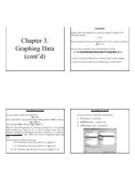
Graphs<br />
In many instances, it is necessary to compose a<br />
plot in order to graphically present the results.<br />
Graphs must be drawn neatly following a specific<br />
format. Figure R.2 shows an acceptable graph<br />
prepared using a computer. There are many<br />
computer programs that have graphing<br />
capabilities. Nevertheless an acceptably drawn<br />
graph has several features <strong>of</strong> note. These features<br />
are summarized next to Figure R.2.<br />
Features <strong>of</strong> note<br />
• Border is drawn about the entire graph.<br />
• Axis labels defined with symbols and<br />
units.<br />
• Grid drawn using major axis divisions.<br />
• Each line is identified using a legend.<br />
• Data points are identified with a<br />
symbol: “ ´” on the Q ac line to denote<br />
data points obtained by experiment.<br />
• The line representing the theoretical<br />
results has no data points represented.<br />
• Nothing is drawn freehand.<br />
• Title is descriptive, rather than<br />
something like Q vs ∆h.<br />
flow rate Q in m 3 /s<br />
0.2<br />
0.15<br />
0.1<br />
0.05<br />
0<br />
Q th<br />
Q ac<br />
0 0.2 0.4 0.6 0.8 1<br />
head loss ∆ h in m<br />
FIGURE R.2. Theoretical and actual volume flow rate<br />
through a venturi meter as a function <strong>of</strong> head loss.<br />
5
CLEANLINESS AND SAFETY<br />
Cleanliness<br />
There are “housekeeping” rules that the user<br />
<strong>of</strong> the laboratory should be aware <strong>of</strong> and abide<br />
by. Equipment in the lab is delicate and each<br />
piece is used extensively for 2 or 3 weeks per<br />
semester. During the remaining time, each<br />
apparatus just sits there, literally collecting dust.<br />
University housekeeping staff are not required to<br />
clean and maintain the equipment. Instead, there<br />
are college technicians who will work on the<br />
equipment when it needs repair, and when they<br />
are notified that a piece <strong>of</strong> equipment needs<br />
attention. It is important, however, that the<br />
equipment stay clean, so that dust will not<br />
accumulate too badly.<br />
The Fluid Mechanics Laboratory contains<br />
equipment that uses water or air as the working<br />
fluid. In some cases, performing an experiment<br />
will inevitably allow water to get on the<br />
equipment and/or the floor. If no one cleaned up<br />
their working area after performing an<br />
experiment, the lab would not be a comfortable or<br />
safe place to work in. No student appreciates<br />
walking up to and working with a piece <strong>of</strong><br />
equipment that another student or group <strong>of</strong><br />
students has left in a mess.<br />
Consequently, students are required to clean<br />
up their area at the conclusion <strong>of</strong> the performance<br />
<strong>of</strong> an experiment. Cleanup will include removal<br />
<strong>of</strong> spilled water (or any liquid), and wiping the<br />
table top on which the equipment is mounted (if<br />
appropriate). The lab should always be as clean<br />
or cleaner than it was when you entered. Cleaning<br />
the lab is your responsibility as a user <strong>of</strong> the<br />
equipment. This is an act <strong>of</strong> courtesy that students<br />
who follow you will appreciate, and that you<br />
will appreciate when you work with the<br />
equipment.<br />
Safety<br />
The layout <strong>of</strong> the equipment and storage<br />
cabinets in the Fluid Mechanics Lab involves<br />
resolving a variety <strong>of</strong> conflicting problems. These<br />
include traffic flow, emergency facilities,<br />
environmental safeguards, exit door locations,<br />
etc. The goal is to implement safety requirements<br />
without impeding egress, but still allowing<br />
adequate work space and necessary informal<br />
communication opportunities.<br />
Distance between adjacent pieces <strong>of</strong><br />
equipment is determined by locations <strong>of</strong> floor<br />
drains, and by the need to allow enough space<br />
around the apparatus <strong>of</strong> interest. Immediate<br />
access to the Safety Cabinet is also considered.<br />
Emergency facilities such as showers, eye wash<br />
fountains, spill kits, fire blankets and the like<br />
are not found in the lab. We do not work with<br />
hazardous materials and such safety facilities<br />
are not necessary. However, waste materials are<br />
generated and they should be disposed <strong>of</strong><br />
properly.<br />
Every effort has been made to create a<br />
positive, clean, safety conscious atmosphere.<br />
Students are encouraged to handle equipment<br />
safely and to be aware <strong>of</strong>, and avoid being<br />
victims <strong>of</strong>, hazardous situations.<br />
6
EXPERIMENT 1<br />
FLUID PROPERTIES: DENSITY AND SURFACE TENSION<br />
There are several properties simple<br />
Newtonian fluids have. They are basic<br />
properties which cannot be calculated for every<br />
fluid, and therefore they must be measured.<br />
These properties are important in making<br />
calculations regarding fluid systems. Measuring<br />
fluid properties, density and viscosity, is the<br />
object <strong>of</strong> this experiment.<br />
W 1<br />
W 2<br />
Part I: Density Measurement.<br />
Equipment<br />
Graduated cylinder or beaker<br />
Liquid whose properties are to be<br />
measured<br />
Hydrometer cylinder<br />
Scale<br />
The density <strong>of</strong> the test fluid is to be found by<br />
weighing a known volume <strong>of</strong> the liquid using the<br />
graduated cylinder or beaker and the scale. The<br />
beaker is weighed empty. The beaker is then<br />
filled to a certain volume according to the<br />
graduations on it and weighed again. The<br />
difference in weight divided by the volume gives<br />
the weight per unit volume <strong>of</strong> the liquid. By<br />
appropriate conversion, the liquid density is<br />
calculated. The mass per unit volume, or the<br />
density, is thus measured in a direct way.<br />
A second method <strong>of</strong> finding density involves<br />
measuring buoyant force exerted on a submerged<br />
object. The difference between the weight <strong>of</strong> an<br />
object in air and the weight <strong>of</strong> the object in liquid<br />
is known as the buoyant force (see Figure 1.1).<br />
FIGURE 1.1. Measuring the buoyant force on an<br />
object with a hanging weight.<br />
Referring to Figure 1.1, the buoyant force B is<br />
found as<br />
B = W 1<br />
- W 2<br />
The buoyant force is equal to the difference<br />
between the weight <strong>of</strong> the object in air and the<br />
weight <strong>of</strong> the object while submerged. Dividing<br />
this difference by the volume displaced gives the<br />
weight per unit volume from which density can be<br />
calculated.<br />
Questions<br />
1. Are the results <strong>of</strong> all the density<br />
measurements in agreement?<br />
2. How does the buoyant force vary with<br />
depth <strong>of</strong> the submerged object? Why?<br />
Part II: Surface Tension Measurement<br />
Equipment<br />
Surface tension meter<br />
Beaker<br />
Test fluid<br />
Surface tension is defined as the energy<br />
required to pull molecules <strong>of</strong> liquid from beneath<br />
the surface to the surface to form a new area. It is<br />
therefore an energy per unit area (F⋅L/L 2 = F/L).<br />
A surface tension meter is used to measure this<br />
energy per unit area and give its value directly. A<br />
schematic <strong>of</strong> the surface tension meter is given in<br />
Figure 1.2.<br />
The platinum-iridium ring is attached to a<br />
balance rod (lever arm) which in turn is attached<br />
to a stainless steel torsion wire. One end <strong>of</strong> this<br />
wire is fixed and the other is rotated. As the wire<br />
is placed under torsion, the rod lifts the ring<br />
slowly out <strong>of</strong> the liquid. The proper technique is<br />
to lower the test fluid container as the ring is<br />
lifted so that the ring remains horizontal. The<br />
force required to break the ring free from the<br />
liquid surface is related to the surface tension <strong>of</strong><br />
the liquid. As the ring breaks free, the gage at<br />
the front <strong>of</strong> the meter reads directly in the units<br />
indicated (dynes/cm) for the given ring. This<br />
reading is called the apparent surface tension and<br />
must be corrected for the ring used in order to<br />
obtain the actual surface tension for the liquid.<br />
The correction factor F can be calculated with the<br />
following equation<br />
7
FIGURE 1.2. A schematic <strong>of</strong> the<br />
surface tension meter.<br />
balance rod<br />
platinum<br />
iridium ring<br />
test liquid<br />
clamp<br />
torsion wire<br />
F = 0.725 + √⎺⎺⎺⎺⎺⎺⎺⎺⎺⎺⎺⎺⎺⎺⎺⎺⎺⎺⎺⎺⎺⎺⎺<br />
0.000 403 3(σ a<br />
/ρ) + 0.045 34 - 1.679(r/R)<br />
where F is the correction factor, σ a is the<br />
apparent surface tension read from the dial<br />
(dyne/cm), ρ is the density <strong>of</strong> the liquid (g/cm 3 ),<br />
and (r/R) for the ring is found on the ring<br />
container. The actual surface tension for the<br />
liquid is given by<br />
σ = Fσ a<br />
8
EXPERIMENT 2<br />
FLUID PROPERTIES: VISCOSITY<br />
One <strong>of</strong> the properties <strong>of</strong> homogeneous liquids<br />
is their resistance to motion. A measure <strong>of</strong> this<br />
resistance is known as viscosity. It can be<br />
measured in different, standardized methods or<br />
tests. In this experiment, viscosity will be<br />
measured with a falling sphere viscometer.<br />
The Falling Sphere Viscometer<br />
When an object falls through a fluid medium,<br />
the object reaches a constant final speed or<br />
terminal velocity. If this terminal velocity is<br />
sufficiently low, then the various forces acting on<br />
the object can be described with exact expressions.<br />
The forces acting on a sphere, for example, that is<br />
falling at terminal velocity through a liquid are:<br />
Weight - Buoyancy - Drag = 0<br />
ρ s g 4 3 πR3 - ρg 4 3 πR3 - 6πµVR = 0<br />
where ρ s and ρ are density <strong>of</strong> the sphere and<br />
liquid respectively, V is the sphere’s terminal<br />
velocity, R is the radius <strong>of</strong> the sphere and µ is<br />
the viscosity <strong>of</strong> the liquid. In solving the<br />
preceding equation, the viscosity <strong>of</strong> the liquid can<br />
be determined. The above expression for drag is<br />
valid only if the following equation is valid:<br />
average the results. With the terminal velocity<br />
<strong>of</strong> this and <strong>of</strong> other spheres measured and known,<br />
the absolute and kinematic viscosity <strong>of</strong> the liquid<br />
can be calculated. The temperature <strong>of</strong> the test<br />
liquid should also be recorded. Use at least three<br />
different spheres. (Note that if the density <strong>of</strong><br />
the liquid is unknown, it can be obtained from any<br />
group who has completed or is taking data on<br />
Experiment 1.)<br />
Questions<br />
1. Should the terminal velocity <strong>of</strong> two<br />
different size spheres be the same?<br />
2. Does a larger sphere have a higher<br />
terminal velocity?<br />
3. Should the viscosity found for two different<br />
size spheres be the same? Why or why not?<br />
4. If different size spheres give different<br />
results for the viscosity, what are the error<br />
sources? Calculate the % error and account<br />
for all known error sources.<br />
5. What are the shortcomings <strong>of</strong> this method?<br />
6. Why should temperature be recorded.<br />
7. Can this method be used for gases?<br />
8. Can this method be used for opaque liquids?<br />
9. Can this method be used for something like<br />
peanut butter, or grease or flour dough?<br />
Why or why not?<br />
ρVD<br />
µ < 1<br />
where D is the sphere diameter. Once the<br />
viscosity <strong>of</strong> the liquid is found, the above ratio<br />
should be calculated to be certain that the<br />
mathematical model gives an accurate<br />
description <strong>of</strong> a sphere falling through the<br />
liquid.<br />
Equipment<br />
Hydrometer cylinder<br />
Scale<br />
Stopwatch<br />
Several small spheres with weight and<br />
diameter to be measured<br />
Test liquid<br />
FIGURE 2.1. Terminal velocity measurement (V =<br />
d/time).<br />
V<br />
d<br />
Drop a sphere into the cylinder liquid and<br />
record the time it takes for the sphere to fall a<br />
certain measured distance. The distance divided<br />
by the measured time gives the terminal velocity<br />
<strong>of</strong> the sphere. Repeat the measurement and<br />
9
EXPERIMENT 3<br />
CENTER OF PRESSURE ON A SUBMERGED<br />
PLANE SURFACE<br />
Submerged surfaces are found in many<br />
engineering applications. Dams, weirs and water<br />
gates are familiar examples <strong>of</strong> submerged<br />
surfaces used to control the flow <strong>of</strong> water. From<br />
the design viewpoint, it is important to have a<br />
working knowledge <strong>of</strong> the forces that act on<br />
submerged surfaces.<br />
A plane surface located beneath the surface<br />
<strong>of</strong> a liquid is subjected to a pressure due to the<br />
height <strong>of</strong> liquid above it, as shown in Figure 3.1.<br />
Increasing pressure varies linearly with<br />
increasing depth resulting in a pressure<br />
distribution that acts on the submerged surface.<br />
The analysis <strong>of</strong> this situation involves<br />
determining a force which is equivalent to the<br />
pressure, and finding the location <strong>of</strong> this force.<br />
FIGURE 3.1. Pressure distribution on a submerged<br />
plane surface and the equivalent force.<br />
For this case, it can be shown that the<br />
equivalent force is:<br />
F = ρgy c<br />
A (3.1)<br />
in which ρ is the liquid density, y c is the distance<br />
from the free surface <strong>of</strong> the liquid to the centroid<br />
<strong>of</strong> the plane, and A is the area <strong>of</strong> the plane in<br />
contact with liquid. Further, the location <strong>of</strong> this<br />
force y F below the free surface is<br />
y F = I xx<br />
y c<br />
A + y c<br />
(3.2)<br />
in which I xx is the second area moment <strong>of</strong> the<br />
plane about its centroid. The experimental<br />
F<br />
y F<br />
verification <strong>of</strong> these equations for force and<br />
distance is the subject <strong>of</strong> this experiment.<br />
Center <strong>of</strong> Pressure Measurement<br />
Equipment<br />
Center <strong>of</strong> Pressure Apparatus<br />
Weights<br />
Figure 3.2 gives a schematic <strong>of</strong> the apparatus<br />
used in this experiment. The torus and balance<br />
arm are placed on top <strong>of</strong> the tank. Note that the<br />
pivot point for the balance arm is the point <strong>of</strong><br />
contact between the rod and the top <strong>of</strong> the tank.<br />
The zeroing weight is adjusted to level the<br />
balance arm. Water is then added to a<br />
predetermined depth. Weights are placed on the<br />
weight hanger to re-level the balance arm. The<br />
amount <strong>of</strong> needed weight and depth <strong>of</strong> water are<br />
then recorded. The procedure is then repeated for<br />
four other depths. (Remember to record the<br />
distance from the pivot point to the free surface<br />
for each case.)<br />
From the depth measurement, the equivalent<br />
force and its location are calculated using<br />
Equations 3.1 and 3.2. Summing moments about the<br />
pivot allows for a comparison between the<br />
theoretical and actual force exerted. Referring to<br />
Figure 3.2, we have<br />
WL<br />
F =<br />
(y + y F )<br />
(3.3)<br />
where y is the distance from the pivot point to<br />
the free surface, y F is the distance from the free<br />
surface to the line <strong>of</strong> action <strong>of</strong> the force F, and L is<br />
the distance from the pivot point to the line <strong>of</strong><br />
action <strong>of</strong> the weight W. Note that both curved<br />
surfaces <strong>of</strong> the torus are circular with centers at<br />
the pivot point. For the report, compare the force<br />
obtained with Equation 3.1 to that obtained with<br />
Equation 3.3. When using Equation 3.3, it will be<br />
necessary to use Equation 3.2 for y F .<br />
Questions<br />
1. In summing moments, why isn't the buoyant<br />
force taken into account?<br />
2. Why isn’t the weight <strong>of</strong> the torus and the<br />
balance arm taken into account?<br />
10
L<br />
level<br />
R i<br />
y<br />
zeroing weight<br />
torus<br />
pivot point<br />
(point <strong>of</strong> contact)<br />
weight<br />
hanger<br />
R o<br />
y F<br />
h<br />
F<br />
w<br />
FIGURE 3.2. A schematic <strong>of</strong> the center <strong>of</strong> pressure apparatus.<br />
11
EXPERIMENT 4<br />
MEASUREMENT OF DIFFERENTIAL PRESSURE<br />
Pressure can be measured in several ways.<br />
Bourdon tube gages, manometers, and transducers<br />
are a few <strong>of</strong> the devices available. Each <strong>of</strong> these<br />
instruments actually measures a difference in<br />
pressure; that is, measures a difference between<br />
the desired reading and some reference pressure,<br />
usually atmospheric. The measurement <strong>of</strong><br />
differential pressure with manometers is the<br />
subject <strong>of</strong> this experiment.<br />
Manometry<br />
A manometer is a device used to measure a<br />
pressure difference and display the reading in<br />
terms <strong>of</strong> height <strong>of</strong> a column <strong>of</strong> liquid. The height<br />
is related to the pressure difference by the<br />
hydrostatic equation.<br />
Figure 4.1 shows a U-tube manometer<br />
connected to two pressure vessels. The manometer<br />
reading is ∆h and the manometer fluid has<br />
density ρ m . One pressure vessel contains a fluid <strong>of</strong><br />
density ρ 1 while the other vessel contains a fluid<br />
<strong>of</strong> density ρ 2 . The pressure difference can be found<br />
by applying the hydrostatic equation to each<br />
limb <strong>of</strong> the manometer. For the left leg,<br />
p 1<br />
p 2<br />
1<br />
p A<br />
z 1<br />
FIGURE 4.1. A U-tube manometer connected to<br />
two pressure vessels.<br />
p 1<br />
+ ρ 1<br />
gz 1<br />
= p A<br />
z 2<br />
Likewise for the right leg,<br />
p 2<br />
+ ρ 2<br />
gz 2<br />
+ ρ m<br />
g∆h = p A<br />
Equating these expressions and solving for the<br />
pressure difference gives<br />
h<br />
p A<br />
m<br />
2<br />
p 1<br />
- p 2<br />
= ρ 2<br />
gz 2<br />
+ ρ 1<br />
gz 1<br />
+ ρ m<br />
g∆h<br />
If the fluids above the manometer liquid are both<br />
gases, then ρ 1 and ρ 2 are small compared to ρ µ .<br />
The above equation then becomes<br />
p 1<br />
- p 2<br />
= ρ m<br />
g∆h<br />
Figure 4.2 is a schematic <strong>of</strong> the apparatus<br />
used in this experiment. It consists <strong>of</strong> three U-tube<br />
manometers, a well-type manometer, a U-<br />
tube/inclined manometer and a differential<br />
pressure gage. There are two tanks (actually, two<br />
capped pieces <strong>of</strong> pipe) to which each manometer<br />
and the gage are connected. The tanks have bleed<br />
valves attached and the tanks are connected<br />
with plastic tubing to a squeeze bulb. The bulb<br />
lines also contain valves. With both bleed valves<br />
closed and with both bulb line valves open, the<br />
bulb is squeezed to pump air from the low pressure<br />
tank to the high pressure tank. The bulb is<br />
squeezed until any <strong>of</strong> the manometers reaches its<br />
maximum reading. Now both valves are closed<br />
and the liquid levels are allowed to settle in<br />
each manometer. The ∆h readings are all<br />
recorded. Next, one or both bleed valves are<br />
opened slightly to release some air into or out <strong>of</strong> a<br />
tank. The liquid levels are again allowed to<br />
settle and the ∆h readings are recorded. The<br />
procedure is to be repeated until 5 different sets <strong>of</strong><br />
readings are obtained. For each set <strong>of</strong> readings,<br />
convert all readings into psi or Pa units, calculate<br />
the average value and the standard deviation.<br />
Before beginning, be sure to zero each manometer<br />
and the gage.<br />
Questions<br />
1. Manometers 1, 2 and 3 are U-tube types and<br />
each contains a different liquid. Manometer<br />
4 is a well-type manometer. Is there an<br />
advantage to using this one over a U-tube<br />
type?<br />
2. Manometer 5 is a combined U/tube/inclined<br />
manometer. What is the advantage <strong>of</strong> this<br />
type?<br />
3. Note that some <strong>of</strong> the manometers use a<br />
liquid which has a specific gravity<br />
different from 1.00, yet the reading is in<br />
inches <strong>of</strong> water. Explain how this is<br />
possible.<br />
4. What advantages or disadvantages does<br />
the gage have over the manometers?<br />
12
5. Is a low value <strong>of</strong> the standard deviation<br />
expected? Why?<br />
6. What does a low standard deviation<br />
imply?<br />
7. In your opinion, which device gives the<br />
most accurate reading. What led you to this<br />
conclusion?<br />
High pressure tank<br />
Low pressure tank<br />
Bleed valves<br />
Gage<br />
U-tube manometers<br />
Well-type<br />
manometer<br />
U-tube/inclined<br />
manometer<br />
FIGURE 4.2. A schematic <strong>of</strong> the apparatus used in this experiment.<br />
13
EXPERIMENT 5<br />
IMPACT OF A JET OF WATER<br />
A jet <strong>of</strong> fluid striking a stationary object<br />
exerts a force on that object. This force can be<br />
measured when the object is connected to a spring<br />
balance or scale. The force can then be related to<br />
the velocity <strong>of</strong> the jet <strong>of</strong> fluid and in turn to the<br />
rate <strong>of</strong> flow. The force developed by a jet stream<br />
<strong>of</strong> water is the subject <strong>of</strong> this experiment.<br />
Impact <strong>of</strong> a Jet <strong>of</strong> Liquid<br />
Equipment<br />
Jet Impact Apparatus<br />
Object plates<br />
Figure 5.1 is a schematic <strong>of</strong> the device used in<br />
this experiment. The device consists <strong>of</strong> a tank<br />
within a tank. The interior tank is supported on a<br />
pivot and has a lever arm attached to it. As<br />
water enters this inner tank, the lever arm will<br />
reach a balance point. At this time, a stopwatch<br />
is started and a weight is placed on the weight<br />
hanger (e.g., 10 lbf). When enough water has<br />
entered the tank (10 lbf), the lever arm will<br />
again balance. The stopwatch is stopped. The<br />
elapsed time divided into the weight <strong>of</strong> water<br />
collected gives the weight or mass flow rate <strong>of</strong><br />
water through the system (lbf/sec, for example).<br />
The outer tank acts as a support for the table<br />
top as well as a sump tank. Water is pumped from<br />
the outer tank to the apparatus resting on the<br />
table top. As shown in Figure 5.1, the impact<br />
apparatus contains a nozzle that produces a high<br />
velocity jet <strong>of</strong> water. The jet is aimed at an object<br />
(such as a flat plate or hemisphere). The force<br />
exerted on the plate causes the balance arm to<br />
which the plate is attached to deflect. A weight<br />
is moved on the arm until the arm balances. A<br />
summation <strong>of</strong> moments about the pivot point <strong>of</strong><br />
the arm allows for calculating the force exerted<br />
by the jet.<br />
Water is fed through the nozzle by means <strong>of</strong><br />
a centrifugal pump. The nozzle emits the water in<br />
a jet stream whose diameter is constant. After the<br />
water strikes the object, the water is channeled to<br />
the weighing tank inside to obtain the weight or<br />
mass flow rate.<br />
The variables involved in this experiment<br />
are listed and their measurements are described<br />
below:<br />
1. Mass rate <strong>of</strong> flow–measured with the<br />
weighing tank inside the sump tank. The<br />
volume flow rate is obtained by dividing<br />
mass flow rate by density: Q = m/ρ.<br />
2. Velocity <strong>of</strong> jet–obtained by dividing volume<br />
flow rate by jet area: V = Q/A. The jet is<br />
cylindrical in shape with a diameter <strong>of</strong> 0.375<br />
in.<br />
3. Resultant force—found experimentally by<br />
summation <strong>of</strong> moments about the pivot point<br />
<strong>of</strong> the balance arm. The theoretical resultant<br />
force is found by use <strong>of</strong> an equation derived by<br />
applying the momentum equation to a control<br />
volume about the plate.<br />
Impact Force Analysis<br />
The total force exerted by the jet equals the<br />
rate <strong>of</strong> momentum loss experienced by the jet after<br />
it impacts the object. For a flat plate, the force<br />
equation is:<br />
F = ρQ2<br />
A<br />
For a hemisphere,<br />
F = 2ρQ2<br />
A<br />
(flat plate)<br />
(hemisphere)<br />
For a cone whose included half angle is α,<br />
F = ρQ2<br />
(1 + cos α) (cone)<br />
A<br />
For your report, derive the appropriate<br />
equation for each object you use. Compose a graph<br />
with volume flow rate on the horizontal axis,<br />
and on the vertical axis, plot the actual and<br />
theoretical force. Use care in choosing the<br />
increments for each axis.<br />
14
pivot<br />
balancing<br />
weight<br />
lever arm with<br />
flat plate attached<br />
water<br />
jet<br />
flat plate<br />
nozzle<br />
drain<br />
flow control<br />
valve<br />
weigh tank<br />
tank pivot<br />
plug<br />
weight hanger<br />
sump tank<br />
motor<br />
pump<br />
FIGURE 5.1. A schematic <strong>of</strong> the jet impact apparatus.<br />
15
EXPERIMENT 6<br />
CRITICAL REYNOLDS NUMBER IN PIPE FLOW<br />
The Reynolds number is a dimensionless ratio<br />
<strong>of</strong> inertia forces to viscous forces and is used in<br />
identifying certain characteristics <strong>of</strong> fluid flow.<br />
The Reynolds number is extremely important in<br />
modeling pipe flow. It can be used to determine<br />
the type <strong>of</strong> flow occurring: laminar or turbulent.<br />
Under laminar conditions the velocity<br />
distribution <strong>of</strong> the fluid within the pipe is<br />
essentially parabolic and can be derived from the<br />
equation <strong>of</strong> motion. When turbulent flow exists,<br />
the velocity pr<strong>of</strong>ile is “flatter” than in the<br />
laminar case because the mixing effect which is<br />
characteristic <strong>of</strong> turbulent flow helps to more<br />
evenly distribute the kinetic energy <strong>of</strong> the fluid<br />
over most <strong>of</strong> the cross section.<br />
In most engineering texts, a Reynolds number<br />
<strong>of</strong> 2 100 is usually accepted as the value at<br />
transition; that is, the value <strong>of</strong> the Reynolds<br />
number between laminar and turbulent flow<br />
regimes. This is done for the sake <strong>of</strong> convenience.<br />
In this experiment, however, we will see that<br />
transition exists over a range <strong>of</strong> Reynolds numbers<br />
and not at an individual point.<br />
The Reynolds number that exists anywhere in<br />
the transition region is called the critical<br />
Reynolds number. Finding the critical Reynolds<br />
number for the transition range that exists in pipe<br />
flow is the subject <strong>of</strong> this experiment.<br />
Critical Reynolds Number Measurement<br />
Equipment<br />
Critical Reynolds Number Determination<br />
Apparatus<br />
Figure 6.1 is a schematic <strong>of</strong> the apparatus<br />
used in this experiment. The constant head tank<br />
provides a controllable, constant flow through<br />
the transparent tube. The flow valve in the tube<br />
itself is an on/<strong>of</strong>f valve, not used to control the<br />
flow rate. Instead, the flow rate through the tube<br />
is varied with the rotameter valve at A. The<br />
head tank is filled with water and the overflow<br />
tube maintains a constant head <strong>of</strong> water. The<br />
liquid is then allowed to flow through one <strong>of</strong> the<br />
transparent tubes at a very low flow rate. The<br />
valve at B controls the flow <strong>of</strong> dye; it is opened<br />
and dye is then injected into the pipe with the<br />
water. The dye injector tube is not to be placed in<br />
the pipe entrance as it could affect the results.<br />
Establish laminar flow by starting with a very<br />
low flow rate <strong>of</strong> water and <strong>of</strong> dye. The injected<br />
dye will flow downstream in a threadlike<br />
pattern for very low flow rates. Once steady state<br />
is achieved, the rotameter valve is opened<br />
slightly to increase the water flow rate. The<br />
valve at B is opened further if necessary to allow<br />
more dye to enter the tube. This procedure <strong>of</strong><br />
increasing flow rate <strong>of</strong> water and <strong>of</strong> dye (if<br />
necessary) is repeated throughout the<br />
experiment.<br />
Establish laminar flow in one <strong>of</strong> the tubes.<br />
Then slowly increase the flow rate and observe<br />
what happens to the dye. Its pattern may<br />
change, yet the flow might still appear to be<br />
laminar. This is the beginning <strong>of</strong> transition.<br />
Continue increasing the flow rate and again<br />
observe the behavior <strong>of</strong> the dye. Eventually, the<br />
dye will mix with the water in a way that will<br />
be recognized as turbulent flow. This point is the<br />
end <strong>of</strong> transition. Transition thus will exist over a<br />
range <strong>of</strong> flow rates. Record the flow rates at key<br />
points in the experiment. Also record the<br />
temperature <strong>of</strong> the water.<br />
The object <strong>of</strong> this procedure is to determine<br />
the range <strong>of</strong> Reynolds numbers over which<br />
transition occurs. Given the tube size, the<br />
Reynolds number can be calculated with:<br />
Re = VD<br />
ν<br />
where V (= Q/A) is the average velocity <strong>of</strong><br />
liquid in the pipe, D is the hydraulic diameter <strong>of</strong><br />
the pipe, and ν is the kinematic viscosity <strong>of</strong> the<br />
liquid.<br />
The hydraulic diameter is calculated from<br />
its definition:<br />
D =<br />
4 x Area<br />
Wetted Perimeter<br />
For a circular pipe flowing full, the hydraulic<br />
diameter equals the inside diameter <strong>of</strong> the pipe.<br />
For a square section, the hydraulic diameter will<br />
equal the length <strong>of</strong> one side (show that this is<br />
the case). The experiment is to be performed for<br />
both round tubes and the square tube. With good<br />
technique and great care, it is possible for the<br />
transition Reynolds number to encompass the<br />
traditionally accepted value <strong>of</strong> 2 100.<br />
16
Questions<br />
1. Can a similar procedure be followed for<br />
gases?<br />
2. Is the Reynolds number obtained at<br />
transition dependent on tube size or shape?<br />
3. Can this method work for opaque liquids?<br />
dye reservoir<br />
drilled partitions<br />
B<br />
transparent tube<br />
on/<strong>of</strong>f valve<br />
rotameter<br />
inlet to<br />
tank<br />
overflow<br />
to drain<br />
FIGURE 6.1. The critical Reynolds number determination apparatus.<br />
A<br />
to drain<br />
17
EXPERIMENT 7<br />
FLUID METERS IN INCOMPRESSIBLE FLOW<br />
There are many different meters used in pipe<br />
flow: the turbine type meter, the rotameter, the<br />
orifice meter, the venturi meter, the elbow meter<br />
and the nozzle meter are only a few. Each meter<br />
works by its ability to alter a certain physical<br />
characteristic <strong>of</strong> the flowing fluid and then<br />
allows this alteration to be measured. The<br />
measured alteration is then related to the flow<br />
rate. A procedure <strong>of</strong> analyzing meters to<br />
determine their useful features is the subject <strong>of</strong><br />
this experiment.<br />
The Venturi Meter<br />
The venturi meter is constructed as shown in<br />
Figure 7.1. It contains a constriction known as the<br />
throat. When fluid flows through the<br />
constriction, it must experience an increase in<br />
velocity over the upstream value. The velocity<br />
increase is accompanied by a decrease in static<br />
pressure at the throat. The difference between<br />
upstream and throat static pressures is then<br />
measured and related to the flow rate. The<br />
greater the flow rate, the greater the pressure<br />
drop ∆p. So the pressure difference ∆h (= ∆p/ρg)<br />
can be found as a function <strong>of</strong> the flow rate.<br />
1<br />
h<br />
2<br />
FIGURE 7.1. A schematic <strong>of</strong> the Venturi meter.<br />
Using the hydrostatic equation applied to<br />
the air-over-liquid manometer <strong>of</strong> Figure 7.1, the<br />
pressure drop and the head loss are related by<br />
(after simplification):<br />
p 1<br />
- p 2<br />
ρg<br />
= ∆h<br />
By combining the continuity equation,<br />
Q = A 1<br />
V 1<br />
= A 2<br />
V 2<br />
with the Bernoulli equation,<br />
p 1<br />
ρ + V 1 2<br />
2 = p 2<br />
ρ + V 2 2<br />
2<br />
and substituting from the hydrostatic equation, it<br />
can be shown after simplification that the<br />
volume flow rate through the venturi meter is<br />
given by<br />
Q = A th 2<br />
√⎺⎺⎺⎺<br />
2g∆h<br />
1 - (D 24<br />
/D 14<br />
)<br />
(7.1)<br />
The preceding equation represents the theoretical<br />
volume flow rate through the venturi meter.<br />
Notice that is was derived from the Bernoulli<br />
equation which does not take frictional effects<br />
into account.<br />
In the venturi meter, there exists small<br />
pressure losses due to viscous (or frictional)<br />
effects. Thus for any pressure difference, the<br />
actual flow rate will be somewhat less than the<br />
theoretical value obtained with Equation 7.1<br />
above. For any ∆h, it is possible to define a<br />
coefficient <strong>of</strong> discharge C v as<br />
C v<br />
= Q ac<br />
Q th<br />
For each and every measured actual flow rate<br />
through the venturi meter, it is possible to<br />
calculate a theoretical volume flow rate, a<br />
Reynolds number, and a discharge coefficient.<br />
The Reynolds number is given by<br />
Re = V 2 D 2<br />
(7.2)<br />
ν<br />
where V 2<br />
is the velocity at the throat <strong>of</strong> the<br />
meter (= Q ac<br />
/A 2<br />
).<br />
The Orifice Meter and<br />
Nozzle-Type Meter<br />
The orifice and nozzle-type meters consist <strong>of</strong><br />
a throttling device (an orifice plate or bushing,<br />
respectively) placed into the flow. (See Figures<br />
7.2 and 7.3). The throttling device creates a<br />
measurable pressure difference from its upstream<br />
to its downstream side. The measured pressure<br />
difference is then related to the flow rate. Like<br />
the venturi meter, the pressure difference varies<br />
with flow rate. Applying Bernoulli’s equation to<br />
points 1 and 2 <strong>of</strong> either meter (Figure 7.2 or Figure<br />
7.3) yields the same theoretical equation as that<br />
for the venturi meter, namely, Equation 7.1. For<br />
any pressure difference, there will be two<br />
associated flow rates for these meters: the<br />
theoretical flow rate (Equation 7.1), and the<br />
18
actual flow rate (measured in the laboratory).<br />
The ratio <strong>of</strong> actual to theoretical flow rate leads<br />
to the definition <strong>of</strong> a discharge coefficient: C o<br />
for<br />
the orifice meter and C n<br />
for the nozzle.<br />
rotor supported<br />
on bearings<br />
(not shown)<br />
to receiver<br />
h<br />
1 2<br />
flow<br />
straighteners<br />
turbine rotor<br />
rotational speed<br />
proportional to<br />
flow rate<br />
FIGURE 7.4. A schematic <strong>of</strong> a turbine-type flow<br />
meter.<br />
FIGURE 7.2. Cross sectional view <strong>of</strong> the orifice<br />
meter.<br />
h<br />
1 2<br />
FIGURE 7.3. Cross sectional view <strong>of</strong> the nozzletype<br />
meter, and a typical nozzle.<br />
For each and every measured actual flow<br />
rate through the orifice or nozzle-type meters, it<br />
is possible to calculate a theoretical volume flow<br />
rate, a Reynolds number and a discharge<br />
coefficient. The Reynolds number is given by<br />
Equation 7.2.<br />
The Turbine-Type Meter<br />
The turbine-type flow meter consists <strong>of</strong> a<br />
section <strong>of</strong> pipe into which a small “turbine” has<br />
been placed. As the fluid travels through the<br />
pipe, the turbine spins at an angular velocity<br />
that is proportional to the flow rate. After a<br />
certain number <strong>of</strong> revolutions, a magnetic pickup<br />
sends an electrical pulse to a preamplifier which<br />
in turn sends the pulse to a digital totalizer. The<br />
totalizer totals the pulses and translates them<br />
into a digital readout which gives the total<br />
volume <strong>of</strong> liquid that travels through the pipe<br />
and/or the instantaneous volume flow rate.<br />
Figure 7.4 is a schematic <strong>of</strong> the turbine type flow<br />
meter.<br />
The Rotameter (Variable Area Meter)<br />
The variable area meter consists <strong>of</strong> a tapered<br />
metering tube and a float which is free to move<br />
inside. The tube is mounted vertically with the<br />
inlet at the bottom. Fluid entering the bottom<br />
raises the float until the forces <strong>of</strong> buoyancy, drag<br />
and gravity are balanced. As the float rises the<br />
annular flow area around the float increases.<br />
Flow rate is indicated by the float position read<br />
against the graduated scale which is etched on<br />
the metering tube. The reading is made usually at<br />
the widest part <strong>of</strong> the float. Figure 7.5 is a sketch<br />
<strong>of</strong> a rotameter.<br />
freely<br />
suspended<br />
float<br />
outlet<br />
tapered, graduated<br />
transparent tube<br />
inlet<br />
FIGURE 7.5. A schematic <strong>of</strong> the rotameter and its<br />
operation.<br />
Rotameters are usually manufactured with<br />
one <strong>of</strong> three types <strong>of</strong> graduated scales:<br />
1. % <strong>of</strong> maximum flow–a factor to convert scale<br />
reading to flow rate is given or determined for<br />
the meter. A variety <strong>of</strong> fluids can be used<br />
with the meter and the only variable<br />
19
encountered in using it is the scale factor. The<br />
scale factor will vary from fluid to fluid.<br />
2. Diameter-ratio type–the ratio <strong>of</strong> cross<br />
sectional diameter <strong>of</strong> the tube to the<br />
diameter <strong>of</strong> the float is etched at various<br />
locations on the tube itself. Such a scale<br />
requires a calibration curve to use the meter.<br />
3. Direct reading–the scale reading shows the<br />
actual flow rate for a specific fluid in the<br />
units indicated on the meter itself. If this<br />
type <strong>of</strong> meter is used for another kind <strong>of</strong> fluid,<br />
then a scale factor must be applied to the<br />
readings.<br />
Experimental Procedure<br />
Equipment<br />
Fluid Meters Apparatus<br />
Stopwatch<br />
The fluid meters apparatus is shown<br />
schematically in Figure 7.6. It consists <strong>of</strong> a<br />
centrifugal pump, which draws water from a<br />
sump tank, and delivers the water to the circuit<br />
containing the flow meters. For nine valve<br />
positions (the valve downstream <strong>of</strong> the pump),<br />
record the pressure differences in each<br />
manometer. For each valve position, measure the<br />
actual flow rate by diverting the flow to the<br />
volumetric measuring tank and recording the time<br />
required to fill the tank to a predetermined<br />
volume. Use the readings on the side <strong>of</strong> the tank<br />
itself. For the rotameter, record the position <strong>of</strong><br />
the float and/or the reading <strong>of</strong> flow rate given<br />
directly on the meter. For the turbine meter,<br />
record the flow reading on the output device.<br />
Note that the venturi meter has two<br />
manometers attached to it. The “inner”<br />
manometer is used to calibrate the meter; that is,<br />
to obtain ∆h readings used in Equation 7.1. The<br />
“outer” manometer is placed such that it reads<br />
the overall pressure drop in the line due to the<br />
presence <strong>of</strong> the meter and its attachment fittings.<br />
We refer to this pressure loss as ∆H (distinctly<br />
different from ∆h). This loss is also a function <strong>of</strong><br />
flow rate. The manometers on the turbine-type<br />
and variable area meters also give the incurred<br />
loss for each respective meter. Thus readings <strong>of</strong><br />
∆H vs Q ac are obtainable. In order to use these<br />
parameters to give dimensionless ratios, pressure<br />
coefficient and Reynolds number are used. The<br />
Reynolds number is given in Equation 7.2. The<br />
pressure coefficient is defined as<br />
C p<br />
= g∆H<br />
V 2 /2<br />
(7.3)<br />
All velocities are based on actual flow rate and<br />
pipe diameter.<br />
The amount <strong>of</strong> work associated with the<br />
laboratory report is great; therefore an informal<br />
group report is required rather than individual<br />
reports. The write-up should consist <strong>of</strong> an<br />
Introduction (to include a procedure and a<br />
derivation <strong>of</strong> Equation 7.1), a Discussion and<br />
Conclusions section, and the following graphs:<br />
1. On the same set <strong>of</strong> axes, plot Q ac vs ∆h and<br />
Q th vs ∆h with flow rate on the vertical<br />
axis for the venturi meter.<br />
2. On the same set <strong>of</strong> axes, plot Q ac vs ∆h and<br />
Q th vs ∆h with flow rate on the vertical<br />
axis for the orifice meter.<br />
3. Plot Q ac<br />
vs Q th<br />
for the turbine type meter.<br />
4. Plot Q ac<br />
vs Q th<br />
for the rotameter.<br />
5. Plot C v vs Re on a log-log grid for the<br />
venturi meter.<br />
6. Plot C o vs Re on a log-log grid for the orifice<br />
meter.<br />
7. Plot ∆H vs Q ac for all meters on the same set<br />
<strong>of</strong> axes with flow rate on the vertical axis.<br />
8. Plot C p vs Re for all meters on the same set<br />
<strong>of</strong> axes (log-log grid) with C p vertical axis.<br />
Questions<br />
1. Referring to Figure 7.2, recall that<br />
Bernoulli's equation was applied to points 1<br />
and 2 where the pressure difference<br />
measurement is made. The theoretical<br />
equation, however, refers to the throat area<br />
for point 2 (the orifice hole diameter)<br />
which is not where the pressure<br />
measurement was made. Explain this<br />
discrepancy and how it is accounted for in<br />
the equation formulation.<br />
2. Which meter in your opinion is the best one<br />
to use?<br />
3. Which meter incurs the smallest pressure<br />
loss? Is this necessarily the one that should<br />
always be used?<br />
4. Which is the most accurate meter?<br />
5. What is the difference between precision<br />
and accuracy?<br />
20
manometer<br />
orifice meter<br />
venturi meter<br />
volumetric<br />
measuring<br />
tank<br />
rotameter<br />
return<br />
sump tank<br />
turbine-type meter<br />
motor pump valve<br />
FIGURE 7.6. A schematic <strong>of</strong> the Fluid Meters Apparatus. (Orifice and Venturi meters: upstream<br />
diameter is 1.025 inches; throat diameter is 0.625 inches.)<br />
21
EXPERIMENT 8<br />
PIPE FLOW<br />
Experiments in pipe flow where the presence<br />
<strong>of</strong> frictional forces must be taken into account are<br />
useful aids in studying the behavior <strong>of</strong> traveling<br />
fluids. Fluids are usually transported through<br />
pipes from location to location by pumps. The<br />
frictional losses within the pipes cause pressure<br />
drops. These pressure drops must be known to<br />
determine pump requirements. Thus a study <strong>of</strong><br />
pressure losses due to friction has a useful<br />
application. The study <strong>of</strong> pressure losses in pipe<br />
flow is the subject <strong>of</strong> this experiment.<br />
Pipe Flow<br />
Equipment<br />
Pipe Flow Test Rig<br />
Figure 8.1 is a schematic <strong>of</strong> the pipe flow test<br />
rig. The rig contains a sump tank which is used as<br />
a water reservoir from which a centrifugal pump<br />
discharges water to the pipe circuit. The circuit<br />
itself consists <strong>of</strong> four different diameter lines and<br />
a return line all made <strong>of</strong> drawn copper tubing. The<br />
circuit contains valves for directing and<br />
regulating the flow to make up various series and<br />
parallel piping combinations. The circuit has<br />
provision for measuring pressure loss through the<br />
use <strong>of</strong> static pressure taps (manometer board not<br />
shown in schematic). Finally, because the circuit<br />
also contains a rotameter, the measured pressure<br />
losses can be obtained as a function <strong>of</strong> flow rate.<br />
As functions <strong>of</strong> the flow rate, measure the<br />
pressure losses in inches <strong>of</strong> water for (as specified<br />
by the instructor):<br />
1. 1 in. copper tube 5. 1 in. 90 T-joint<br />
2. 3 /4-in. copper tube 6. 1 in. 90 elbow (ell)<br />
3. 1 /2-in copper tube 7. 1 in. gate valve<br />
4. 3 /8 in copper tube 8. 3 /4-in gate valve<br />
• The instructor will specify which <strong>of</strong> the<br />
pressure loss measurements are to be taken.<br />
• Open and close the appropriate valves on the<br />
apparatus to obtain the desired flow path.<br />
• Use the valve closest to the pump on its<br />
downstream side to vary the volume flow<br />
rate.<br />
• With the pump on, record the assigned<br />
pressure drops and the actual volume flow<br />
rate from the rotameter.<br />
• Using the valve closest to the pump, change<br />
the volume flow rate and again record the<br />
pressure drops and the new flow rate value.<br />
• Repeat this procedure until 9 different<br />
volume flow rates and corresponding pressure<br />
drop data have been recorded.<br />
With pressure loss data in terms <strong>of</strong> ∆h, the<br />
friction factor can be calculated with<br />
2g∆h<br />
f =<br />
V 2 (L/D)<br />
It is customary to graph the friction factor as a<br />
function <strong>of</strong> the Reynolds number:<br />
Re = VD<br />
ν<br />
The f vs Re graph, called a Moody Diagram is<br />
traditionally drawn on a log-log grid. The graph<br />
also contains a third variable known as the<br />
roughness coefficient ε/D. For this experiment<br />
the roughness factor ε is that for drawn tubing.<br />
Where fittings are concerned, the loss<br />
incurred by the fluid is expressed in terms <strong>of</strong> a loss<br />
coefficient K. The loss coefficient for any fitting<br />
can be calculated with<br />
K =<br />
∆ h<br />
V 2 /2g<br />
where ∆h is the pressure (or head) loss across the<br />
fitting. Values <strong>of</strong> K as a function <strong>of</strong> Q ac are to be<br />
obtained in this experiment.<br />
For the report, calculate friction factor f and<br />
graph it as a function <strong>of</strong> Reynolds number Re for<br />
items 1 through 4 above as appropriate. Compare<br />
to a Moody diagram. Also calculate the loss<br />
coefficient for items 5 through 8 above as<br />
appropriate, and determine if the loss coefficient<br />
K varies with flow rate or Reynolds number.<br />
Compare your K values to published ones.<br />
Note that gate valves can have a number <strong>of</strong><br />
open positions. For purposes <strong>of</strong> comparison it is<br />
<strong>of</strong>ten convenient to use full, half or one-quarter<br />
open.<br />
22
otameter<br />
tank<br />
valve<br />
motor<br />
static pressure tap<br />
pump<br />
FIGURE 8.1. Schematic <strong>of</strong> the pipe friction apparatus.<br />
23
EXPERIMENT 9<br />
PRESSURE DISTRIBUTION ABOUT A CIRCULAR CYLINDER<br />
In many engineering applications, it may be<br />
necessary to examine the phenomena occurring<br />
when an object is inserted into a flow <strong>of</strong> fluid. The<br />
wings <strong>of</strong> an airplane in flight, for example, may<br />
be analyzed by considering the wings stationary<br />
with air moving past them. Certain forces are<br />
exerted on the wing by the flowing fluid that<br />
tend to lift the wing (called the lift force) and to<br />
push the wing in the direction <strong>of</strong> the flow (drag<br />
force). Objects other than wings that are<br />
symmetrical with respect to the fluid approach<br />
direction, such as a circular cylinder, will<br />
experience no lift, only drag.<br />
Drag and lift forces are caused by the<br />
pressure differences exerted on the stationary<br />
object by the flowing fluid. Skin friction between<br />
the fluid and the object contributes to the drag<br />
force but in many cases can be neglected. The<br />
measurement <strong>of</strong> the pressure distribution existing<br />
around a stationary cylinder in an air stream to<br />
find the drag force is the object <strong>of</strong> this<br />
experiment.<br />
Consider a circular cylinder immersed in a<br />
uniform flow. The streamlines about the cylinder<br />
are shown in Figure 9.1. The fluid exerts pressure<br />
on the front half <strong>of</strong> the cylinder in an amount<br />
that is greater than that exerted on the rear<br />
half. The difference in pressure multiplied by the<br />
projected frontal area <strong>of</strong> the cylinder gives the<br />
drag force due to pressure (also known as form<br />
drag). Because this drag is due primarily to a<br />
pressure difference, measurement <strong>of</strong> the pressure<br />
distribution about the cylinder allows for finding<br />
the drag force experimentally. A typical pressure<br />
distribution is given in Figure 9.2. Shown in<br />
Figure 9.2a is the cylinder with lines and<br />
arrowheads. The length <strong>of</strong> the line at any point<br />
on the cylinder surface is proportional to the<br />
pressure at that point. The direction <strong>of</strong> the<br />
arrowhead indicates that the pressure at the<br />
respective point is greater than the free stream<br />
pressure (pointing toward the center <strong>of</strong> the<br />
cylinder) or less than the free stream pressure<br />
(pointing away). Note the existence <strong>of</strong> a<br />
separation point and a separation region (or<br />
wake). The pressure in the back flow region is<br />
nearly the same as the pressure at the point <strong>of</strong><br />
separation. The general result is a net drag force<br />
equal to the sum <strong>of</strong> the forces due to pressure<br />
acting on the front half (+) and on the rear half<br />
(-) <strong>of</strong> the cylinder. To find the drag force, it is<br />
necessary to sum the components <strong>of</strong> pressure at<br />
each point in the flow direction. Figure 9.2b is a<br />
graph <strong>of</strong> the same data as that in Figure 9.2a<br />
except that 9.2b is on a linear grid.<br />
Freestream<br />
Velocity V<br />
Stagnation<br />
Streamline<br />
Wake<br />
FIGURE 9.1. Streamlines <strong>of</strong> flow about a circular<br />
cylinder.<br />
separation<br />
point<br />
p<br />
0 30 60 90 120 150 180<br />
separation<br />
point<br />
(a) Polar Coordinate Graph<br />
(b) Linear Graph<br />
FIGURE 9.2. Pressure distribution around a circular cylinder placed in a uniform flow.<br />
24
Pressure Measurement<br />
Equipment<br />
A Wind Tunnel<br />
A Right Circular Cylinder with Pressure<br />
Taps<br />
Figure 9.3 is a schematic <strong>of</strong> a wind tunnel. It<br />
consists <strong>of</strong> a nozzle, a test section, a diffuser and a<br />
fan. Flow enters the nozzle and passes through<br />
flow straighteners and screens. The flow is<br />
directed through a test section whose walls are<br />
made <strong>of</strong> a transparent material, usually<br />
Plexiglas or glass. An object is placed in the test<br />
section for observation. Downstream <strong>of</strong> the test<br />
section is the diffuser followed by the fan. In the<br />
tunnel that is used in this experiment, the test<br />
section is rectangular and the fan housing is<br />
circular. Thus one function <strong>of</strong> the diffuser is to<br />
gradually lead the flow from a rectangular<br />
section to a circular one.<br />
Figure 9.4 is a schematic <strong>of</strong> the side view <strong>of</strong><br />
the circular cylinder. The cylinder is placed in<br />
the test section <strong>of</strong> the wind tunnel which is<br />
operated at a preselected velocity. The pressure<br />
tap labeled as #1 is placed at 0° directly facing<br />
the approach flow. The pressure taps are<br />
attached to a manometer board. Only the first 18<br />
taps are connected because the expected pr<strong>of</strong>ile is<br />
symmetric about the 0° line. The manometers will<br />
provide readings <strong>of</strong> pressure at 10° intervals<br />
about half the cylinder. For two different<br />
approach velocities, measure and record the<br />
pressure distribution about the circular cylinder.<br />
Plot the pressure distribution on polar coordinate<br />
graph paper for both cases. Also graph pressure<br />
difference (pressure at the point <strong>of</strong> interest minus<br />
the free stream pressure) as a function <strong>of</strong> angle θ<br />
on linear graph paper. Next, graph ∆p cosθ vs θ<br />
(horizontal axis) on linear paper and determine<br />
the area under the curve by any convenient<br />
method (counting squares or a numerical<br />
technique).<br />
The drag force can be calculated by<br />
integrating the flow-direction-component <strong>of</strong> each<br />
pressure over the area <strong>of</strong> the cylinder:<br />
π<br />
D f<br />
= 2RL<br />
0<br />
∫ ∆p cosθdθ<br />
The above expression states that the drag force is<br />
twice the cylinder radius (2R) times the cylinder<br />
length (L) times the area under the curve <strong>of</strong> ∆p<br />
cosθ vs θ.<br />
Drag data are usually expressed as drag<br />
coefficient C D<br />
vs Reynolds number Re. The drag<br />
coefficient is defined as<br />
D f<br />
C D<br />
=<br />
ρV 2 A/2<br />
The Reynolds number is<br />
Re = ρVD<br />
µ<br />
inlet flow<br />
straighteners<br />
nozzle<br />
test section<br />
diffuser<br />
fan<br />
FIGURE 9.3. A schematic <strong>of</strong> the wind tunnel used in this experiment.<br />
25
where V is the free stream velocity (upstream <strong>of</strong><br />
the cylinder), A is the projected frontal area <strong>of</strong><br />
the cylinder (2RL), D is the cylinder diameter, ρ<br />
is the air density and µ is the air viscosity.<br />
Compare the results to those found in texts.<br />
60<br />
90<br />
120<br />
0<br />
30<br />
static pressure<br />
taps attach to<br />
manometers<br />
150<br />
180<br />
FIGURE 9.4. Schematic <strong>of</strong> the experimental<br />
apparatus used in this experiment.<br />
26
EXPERIMENT 10<br />
DRAG FORCE DETERMINATION<br />
An object placed in a uniform flow is acted<br />
upon by various forces. The resultant <strong>of</strong> these<br />
forces can be resolved into two force components,<br />
parallel and perpendicular to the main flow<br />
direction. The component acting parallel to the<br />
flow is known as the drag force. It is a function <strong>of</strong><br />
a skin friction effect and an adverse pressure<br />
gradient. The component perpendicular to the<br />
flow direction is the lift force and is caused by a<br />
pressure distribution which results in a lower<br />
pressure acting over the top surface <strong>of</strong> the object<br />
than at the bottom. If the object is symmetric<br />
with respect to the flow direction, then the lift<br />
force will be zero and only a drag force will exist.<br />
Measurement <strong>of</strong> the drag force acting on an object<br />
immersed in the uniform flow <strong>of</strong> a fluid is the<br />
subject <strong>of</strong> this experiment.<br />
Equipment<br />
Subsonic Wind Tunnel<br />
Objects<br />
A description <strong>of</strong> a subsonic wind tunnel is<br />
given in Experiment 9 and is shown schematically<br />
in Figure 9.3. The fan at the end <strong>of</strong> the tunnel<br />
draws in air at the inlet. An object is mounted on a<br />
stand that is pre calibrated to read lift and drag<br />
forces exerted by the fluid on the object. A<br />
schematic <strong>of</strong> the test section is shown in Figure<br />
10.1. The velocity <strong>of</strong> the flow at the test section is<br />
also pre calibrated. The air velocity past the<br />
object can be controlled by changing the angle <strong>of</strong><br />
the inlet vanes located within the fan housing.<br />
Thus air velocity, lift force and drag force are<br />
read directly from the tunnel instrumentation.<br />
There are a number <strong>of</strong> objects that are<br />
available for use in the wind tunnel. These<br />
include a disk, a smooth surfaced sphere, a rough<br />
surface sphere, a hemisphere facing upstream,<br />
and a hemisphere facing downstream. For<br />
whichever is assigned, measure drag on the object<br />
as a function <strong>of</strong> velocity.<br />
Data on drag vs velocity are usually graphed<br />
in dimensionless terms. The drag force D f is<br />
customarily expressed in terms <strong>of</strong> the drag<br />
coefficient C D (a ratio <strong>of</strong> drag force to kinetic<br />
energy):<br />
in which ρ is the fluid density, V is the free<br />
stream velocity, and A is the projected frontal<br />
area <strong>of</strong> the object. Traditionally, the drag<br />
coefficient is graphed as a function <strong>of</strong> the<br />
Reynolds number, which is defined as<br />
Re = VD<br />
ν<br />
where D is a characteristic length <strong>of</strong> the object<br />
and ν is the kinematic viscosity <strong>of</strong> the fluid. For<br />
each object assigned, graph drag coefficient vs<br />
Reynolds number and compare your results to<br />
those published in texts. Use log-log paper if<br />
appropriate.<br />
Questions<br />
1. How does the mounting piece affect the<br />
readings?<br />
2. How do you plan to correct for its effect, if<br />
necessary?<br />
uniform flow<br />
lift force<br />
measurement<br />
object<br />
mounting stand<br />
drag force<br />
measurement<br />
FIGURE 10.1. Schematic <strong>of</strong> an object mounted in<br />
the test section <strong>of</strong> the wind tunnel.<br />
D f<br />
C D<br />
=<br />
ρV 2 A/2<br />
27
EXPERIMENT 11<br />
ANALYSIS OF AN AIRFOIL<br />
A wing placed in the uniform flow <strong>of</strong> an<br />
airstream will experience lift and drag forces.<br />
Each <strong>of</strong> these forces is due to a pressure<br />
difference. The lift force is due to the pressure<br />
difference that exists between the lower and<br />
upper surfaces. This phenomena is illustrated in<br />
Figure 11.1. As indicated the airfoil is immersed<br />
in a uniform flow. If pressure could be measured at<br />
selected locations on the surface <strong>of</strong> the wing and<br />
the results graphed, the pr<strong>of</strong>ile in Figure 11.1<br />
would result. Each pressure measurement is<br />
represented by a line with an arrowhead. The<br />
length <strong>of</strong> each line is proportional to the<br />
magnitude <strong>of</strong> the pressure at the point. The<br />
direction <strong>of</strong> the arrow (toward the horizontal<br />
axis or away from it) represents whether the<br />
pressure at the point is less than or greater than<br />
the free stream pressure measured far upstream <strong>of</strong><br />
the wing.<br />
Experiment I<br />
Mount the wing with pressure taps in the<br />
tunnel and attach the tube ends to manometers.<br />
Select a wind speed and record the pressure<br />
distribution for a selected angle <strong>of</strong> attack (as<br />
assigned by the instructor). Plot pressure vs chord<br />
length as in Figure 11.1, showing the vertical<br />
component <strong>of</strong> each pressure acting on the upper<br />
surface and on the lower surface. Determine<br />
where separation occurs for each case.<br />
Mount the second wing on the lift and drag<br />
balance (Figure 11.2). For the same wind speed<br />
and angle <strong>of</strong> attack, measure lift and drag exerted<br />
on the wing.<br />
lift<br />
c<br />
drag<br />
c<br />
uniform flow<br />
mounting stand<br />
stagnation<br />
point<br />
C p<br />
pressure<br />
coefficient<br />
negative pressure<br />
gradient on upper<br />
surface<br />
lift force<br />
measurement<br />
drag force<br />
measurement<br />
stagnation<br />
point<br />
chord, c<br />
positive pressure<br />
on lower surface<br />
FIGURE 11.2. Schematic <strong>of</strong> lift and drag<br />
measurement in a test section.<br />
FIGURE 11.1. Streamlines <strong>of</strong> flow about a wing<br />
and the resultant pressure distribution.<br />
Lift and Drag Measurements for a Wing<br />
Equipment<br />
Wind Tunnel (See Figure 9.3)<br />
Wing with Pressure Taps<br />
Wing for Attachment to Lift & Drag<br />
Instruments (See Figure 11.2)<br />
The wing with pressure taps provided<br />
pressure at selected points on the surface <strong>of</strong> the<br />
wing. Use the data obtained and sum the<br />
horizontal component <strong>of</strong> each pressure to obtain<br />
the drag force. Compare to the results obtained<br />
with the other wing. Use the data obtained and<br />
sum the vertical component <strong>of</strong> each pressure to<br />
obtain the lift force. Compare the results<br />
obtained with the other wing. Calculate %<br />
errors.<br />
28
Experiment II<br />
For a number <strong>of</strong> wings, lift and drag data<br />
vary only slightly with Reynolds number and<br />
therefore if lift and drag coefficients are graphed<br />
as a function <strong>of</strong> Reynolds number, the results are<br />
not that meaningful. A more significant<br />
representation <strong>of</strong> the results is given in what is<br />
known as a polar diagram for the wing. A polar<br />
diagram is a graph on a linear grid <strong>of</strong> lift<br />
coefficient (vertical axis) as a function <strong>of</strong> drag<br />
coefficient. Each data point on the graph<br />
corresponds to a different angle <strong>of</strong> attack, all<br />
measured at one velocity (Reynolds number).<br />
Referring to Figure 11.2 (which is the<br />
experimental setup here), the angle <strong>of</strong> attack α is<br />
measured from a line parallel to the chord c to a<br />
line that is parallel to the free stream velocity.<br />
If so instructed, obtain lift force, drag force and<br />
angle <strong>of</strong> attack data using a pre selected velocity.<br />
Allow the angle <strong>of</strong> attack to vary from a negative<br />
angle to the stall point and beyond. Obtain data<br />
at no less than 9 angles <strong>of</strong> attack. Use the data to<br />
produce a polar diagram.<br />
Analysis<br />
Lift and drag data are usually expressed in<br />
dimensionless terms using lift coefficient and drag<br />
coefficient. The lift coefficient is defined as<br />
L f<br />
C L<br />
=<br />
ρV 2 A/2<br />
where L f is the lift force, ρ is the fluid density, V<br />
is the free stream velocity far upstream <strong>of</strong> the<br />
wing, and A is the area <strong>of</strong> the wing when seen<br />
from a top view perpendicular to the chord<br />
length c. The drag coefficient is defined as<br />
D f<br />
C D<br />
=<br />
ρV 2 A/2<br />
in which D f<br />
is the drag force.<br />
29
EXPERIMENT 12<br />
OPEN CHANNEL FLOW—SLUICE GATE<br />
Liquid motion in a duct where a surface <strong>of</strong> the<br />
fluid is exposed to the atmosphere is called open<br />
channel flow. In the laboratory, open channel<br />
flow experiments can be used to simulate flow in a<br />
river, in a spillway, in a drainage canal or in a<br />
sewer. Such modeled flows can include flow over<br />
bumps or through dams, flow through a venturi<br />
flume or under a partially raised gate (a sluice<br />
gate). The last example, flow under a sluice gate,<br />
is the subject <strong>of</strong> this experiment.<br />
Flow Through a Sluice Gate<br />
Equipment<br />
Open Channel Flow Apparatus<br />
Sluice Gate Model<br />
Figure 12.1 shows a schematic <strong>of</strong> the side<br />
view <strong>of</strong> the sluice gate. Flow upstream <strong>of</strong> the gate<br />
has a depth h o while downstream the depth is h.<br />
The objective <strong>of</strong> the analysis is to formulate an<br />
equation to relate the volume flow rate through<br />
(or under) the gate to the upstream and<br />
downstream depths.<br />
sluice gate<br />
p atm<br />
h o<br />
hand crank<br />
direction <strong>of</strong><br />
movement<br />
h<br />
p atm<br />
FIGURE 12.1. Schematic <strong>of</strong> flow under a sluice<br />
gate.<br />
The flow rate through the gate is maintained at<br />
nearly a constant value. For various raised<br />
positions <strong>of</strong> the sluice gate, different liquid<br />
heights h o and h will result. Applying the<br />
Bernoulli equation to flow about the gate gives<br />
p 0<br />
ρg + V 0 2<br />
2g + h 0 = p ρg + V2<br />
2g + h<br />
Pressures at the free surface are both equal to<br />
atmospheric pressure, so they cancel. Rearranging<br />
gives<br />
h 0 = V2<br />
2g - V 0 2<br />
2g +h<br />
In terms <strong>of</strong> flow rate, the velocities are written as<br />
V 0 = Q A = Q<br />
bh 0<br />
V = Q bh<br />
where b is the channel width at the gate.<br />
Substituting into the Bernoulli Equation and<br />
simplifying gives<br />
h 0 = Q2<br />
2gb 2 ⎝ ⎛ 1<br />
h ⎠ ⎞ 2 - 1<br />
h<br />
2 + h<br />
0<br />
Dividing by h 0 ,<br />
Q<br />
1 =<br />
2<br />
2gb 2 h 0 ⎝ ⎛ 1<br />
h ⎠ ⎞<br />
2 - 1<br />
h<br />
2 + h 0 h 0<br />
Rearranging further,<br />
Q 2<br />
⎛1 - h ⎞ =<br />
⎝ h 0 ⎠ 2gb 2 h 2 h 0 ⎝ ⎛ 1 - h 2<br />
h ⎠ ⎞ 2 0<br />
Multiplying both sides by h 2 /h 0 2 , and continuing<br />
to simplify, we finally obtain<br />
h 2 /h<br />
2 0 Q<br />
=<br />
2<br />
1 + h/h 0 2gb 2 h<br />
3 0<br />
here Q is the theoretical volume flow rate. The<br />
right hand side <strong>of</strong> this equation is recognized as<br />
1/2 <strong>of</strong> the upstream Froude number. So by<br />
measuring the depth <strong>of</strong> liquid before and after<br />
the sluice gate, the theoretical flow rate can be<br />
calculated with the above equation. The<br />
theoretical flow rate can then be compared to the<br />
actual flow rate obtained by measurements using<br />
the orifice meters.<br />
For 9 different raised positions <strong>of</strong> the sluice<br />
gate, measure the upstream and downstream<br />
depths and calculate the actual flow rate. In<br />
addition, calculate the upstream Froude number<br />
for each case and determine its value for<br />
maximum flow conditions. Graph h/h 0 (vertical<br />
30
axis) versus (Q 2 /b 2 h 0 3 g). Determine h/h 0<br />
corresponding to maximum flow. Note that h/h 0<br />
varies from 0 to 1.<br />
Figure 12.2 is a sketch <strong>of</strong> the open channel<br />
flow apparatus. It consists <strong>of</strong> a sump tank with a<br />
pump/motor combination on each side. Each pump<br />
draws in water from the sump tank and<br />
discharges it through the discharge line to<br />
calibrated orifice meters and then to the head<br />
tank. Each orifice meter is connected to its own<br />
manometer. Use <strong>of</strong> the calibration curve<br />
(provided by the instructor) allows for finding<br />
the actual flow rate into the channel. The head<br />
tank and flow channel have sides made <strong>of</strong><br />
Plexiglas. Water flows downstream in the<br />
channel past the object <strong>of</strong> interest (in this case a<br />
sluice gate) and then is routed back to the sump<br />
tank.<br />
Questions<br />
1. For the required report, derive the sluice<br />
gate equation in detail.<br />
2. What if it was assumed that V 0
EXPERIMENT 13<br />
OPEN CHANNEL FLOW OVER A WEIR<br />
Flow meters used in pipes introduce an<br />
obstruction into the flow which results in a<br />
measurable pressure drop that in turn is related to<br />
the volume flow rate. In an open channel, flow<br />
rate can be measured similarly by introducing an<br />
obstruction into the flow. A simple obstruction,<br />
called a weir, consists <strong>of</strong> a vertical plate<br />
extending the entire width <strong>of</strong> the channel. The<br />
plate may have an opening, usually rectangular,<br />
trapezoidal, or triangular. Other configurations<br />
exist and all are about equally effective. The use<br />
<strong>of</strong> a weir to measure flow rate in an open channel<br />
is the subject <strong>of</strong> this experiment.<br />
Flow Over a Weir<br />
Equipment<br />
Open Channel Flow Apparatus (See<br />
Figure 12.1)<br />
Several Weirs<br />
The open channel flow apparatus allows for<br />
the insertion <strong>of</strong> a weir and measurement <strong>of</strong> liquid<br />
depths. The channel is fed by two centrifugal<br />
pumps. Each pump has a discharge line which<br />
contains an orifice meter attached to a<br />
manometer. The pressure drop reading from the<br />
manometers and a calibration curve provide the<br />
means for determining the actual flow rate into<br />
the channel.<br />
Figure 13.1 is a sketch <strong>of</strong> the side and<br />
upstream view <strong>of</strong> a 90 degree (included angle) V-<br />
notch weir. Analysis <strong>of</strong> this weir is presented<br />
here for illustrative purposes. Note that<br />
upstream depth measurements are made from the<br />
lowest point <strong>of</strong> the weir over which liquid flows.<br />
This is the case for the analysis <strong>of</strong> all<br />
conventional weirs. A coordinate system is<br />
imposed whose origin is at the intersection <strong>of</strong> the<br />
free surface and a vertical line extending upward<br />
from the vertex <strong>of</strong> the V-notch. We select an<br />
element that is dy thick and extends the entire<br />
width <strong>of</strong> the flow cross section. The velocity <strong>of</strong><br />
the liquid through this element is found by<br />
applying Bernoulli's equation:<br />
p a<br />
ρ + V o 2<br />
2 + gh = p a<br />
ρ + V2<br />
+ g(h - y)<br />
2<br />
Note that in pipe flow, pressure remained in the<br />
equation when analyzing any <strong>of</strong> the differential<br />
pressure meters (orifice or venturi meters). In open<br />
channel flows, the pressure terms represents<br />
atmospheric pressure and cancel from the<br />
Bernoulli equation. The liquid height is<br />
therefore the only measurement required here.<br />
From the above equation, assuming V o<br />
negligible:<br />
V = √⎺⎺⎺2gy (13.1)<br />
Equation 13.1 is the starting point in the analysis<br />
<strong>of</strong> all weirs. The incremental flow rate <strong>of</strong> liquid<br />
through layer dy is:<br />
dQ = 2Vxdy = √⎺⎺⎺2gy(2x)dy<br />
From the geometry <strong>of</strong> the V-notch and with<br />
respect to the coordinate axes, we have y = h - x.<br />
V o<br />
p a<br />
h<br />
V<br />
p a<br />
y axis<br />
y<br />
dy<br />
x<br />
FIGURE 13.1. Side and upstream views <strong>of</strong> a 90° V-notch weir.<br />
x axis<br />
32
Therefore,<br />
Q = ∫<br />
0<br />
Integration gives<br />
h<br />
(2√⎺⎺2g)y 1/2 (h - y)dy<br />
Q th = 8 15 √⎺⎺ 2g h 5/2 =Ch 5/2 (13.2)<br />
where C is a constant. The above equation<br />
represents the ideal or theoretical flow rate <strong>of</strong><br />
liquid over the V-notch weir. The actual<br />
discharge rate is somewhat less due to frictional<br />
and other dissipative effects. As with pipe<br />
meters, we introduce a discharge coefficient<br />
defined as:<br />
C' = Q ac<br />
Q th<br />
The equation that relates the actual volume flow<br />
rate to the upstream height then is<br />
Q ac<br />
= C'Ch 5/2<br />
It is convenient to combine the effects <strong>of</strong> the<br />
constant C and the coefficient C’ into a single<br />
coefficient C vn for the V-notch weir. Thus we<br />
reformulate the previous two equations to obtain:<br />
C vn ≈ Q ac<br />
Q th<br />
(13.3)<br />
Q ac<br />
= C vn h 5/2 (13.4)<br />
Each type <strong>of</strong> weir will have its own coefficient.<br />
Calibrate each <strong>of</strong> the weirs assigned by the<br />
instructor for 7 different upstream height<br />
measurements. Use the flow rate chart provided<br />
with the open channel flow apparatus to obtain<br />
the actual flow rate. Derive an appropriate<br />
equation for each weir used (similar to Equation<br />
13.4) above. Determine the coefficient applicable<br />
for each weir tested. List the assumptions made<br />
in each derivation. Discuss the validity <strong>of</strong> each<br />
assumption, pointing out where they break down.<br />
Graph upstream height vs actual and theoretical<br />
volume flow rates. Plot the coefficient <strong>of</strong><br />
discharge (as defined in Equation 13.3) as a<br />
function <strong>of</strong> the upstream Froude number.<br />
FIGURE 13.2. Other types <strong>of</strong> weirs–semicircular, contracted and suppressed.<br />
33
EXPERIMENT 14<br />
OPEN CHANNEL FLOW—HYDRAULIC JUMP<br />
When spillways or other similar open<br />
channels are opened by the lifting <strong>of</strong> a gate,<br />
liquid passing below the gate has a high velocity<br />
and an associated high kinetic energy. Due to the<br />
erosive properties <strong>of</strong> a high velocity fluid, it<br />
may be desirable to convert the high kinetic<br />
energy (e.g. high velocity) to a high potential<br />
energy (e.g., a deeper stream). The problem then<br />
becomes one <strong>of</strong> rapidly varying the liquid depth<br />
over a short channel length. Rapidly varied flow<br />
<strong>of</strong> this type produces what is known as a<br />
hydraulic jump.<br />
Consider a horizontal, rectangular open<br />
channel <strong>of</strong> width b, in which a hydraulic jump<br />
has developed. Figure 14.1 shows a side view <strong>of</strong> a<br />
hydraulic jump. Figure 14.1 also shows the depth<br />
<strong>of</strong> liquid upstream <strong>of</strong> the jump to be h 1<br />
, and a<br />
downstream depth <strong>of</strong> h 2<br />
. Pressure distributions<br />
upstream and downstream <strong>of</strong> the jump are drawn<br />
in as well. Because the jump occurs over a very<br />
short distance, frictional effects can be neglected.<br />
A force balance would therefore include only<br />
pressure forces. Applying the momentum equation<br />
in the flow direction gives:<br />
p 1<br />
A 1<br />
- p 2<br />
A 2<br />
= ρQ(V 2<br />
- V 1<br />
)<br />
Pressure in the above equation represents the<br />
pressure that exists at the centroid <strong>of</strong> the cross<br />
section. Thus p = ρg(h/2). With a rectangular<br />
cross section <strong>of</strong> width b (A = bh), the above<br />
equation becomes<br />
h 1<br />
g<br />
2 (h 1 b) - h 2 g<br />
2 (h 2 b) = Q(V 2 - V 1 )<br />
From continuity, A 1<br />
V 1<br />
= A 2<br />
V 2<br />
= Q. Combining and<br />
rearranging,<br />
h<br />
2<br />
1<br />
- h<br />
2<br />
2<br />
= Q 2<br />
2 gb 2 ⎝ ⎛ 1<br />
- 1 h ⎠ ⎞<br />
2<br />
h 1<br />
Simplifying,<br />
h 2<br />
2<br />
+ h 2<br />
h 1<br />
- 2<br />
Q 2<br />
gb 2 h 1<br />
= 0<br />
Solving for the downstream height yields one<br />
physically (nonnegative) possible solution:<br />
h 2<br />
= - h 1<br />
2 √⎺⎺⎺⎺<br />
+ 2Q 2<br />
4<br />
gb 2 h 1<br />
+ h 1 2<br />
from which the downstream height can be found.<br />
By applying Bernoulli’s Equation along the free<br />
surface, the energy lost irreversibly can be<br />
calculated as<br />
Lost Energy = E =<br />
g(h 2<br />
- h 1<br />
) 3<br />
4h 2<br />
h 1<br />
and the rate <strong>of</strong> energy loss is<br />
dW<br />
dt = ρQE<br />
The above equations are adequate to properly<br />
describe a hydraulic jump.<br />
Hydraulic Jump Measurements<br />
Equipment<br />
Open Channel Flow Apparatus (Figure 12.1)<br />
The channel can be used in either a<br />
horizontal or a sloping configuration. The device<br />
contains two pumps which discharge water<br />
through calibrated orifice meters connected to<br />
manometers. The device also contains on the<br />
channel bottom two forward facing brass tubes.<br />
Each tube is connected to a vertical Plexiglas<br />
tube. The height <strong>of</strong> the water in either <strong>of</strong> these<br />
tubes represents the energy level at the<br />
respective tube location. The difference in height<br />
is the actual lost energy (E) for the jump <strong>of</strong><br />
interest.<br />
FIGURE 14.1. Schematic <strong>of</strong> a<br />
hydraulic jump in an open<br />
channel.<br />
h 1<br />
V 2<br />
V 1<br />
p 1<br />
p 2<br />
h 2<br />
34
Develop a hydraulic jump in the channel;<br />
record upstream and downstream heights,<br />
manometer readings (from which the actual<br />
volume flow rate is obtained) and the lost energy<br />
E. By varying the flow rate, upstream height,<br />
downstream height and/or the channel slope,<br />
record measurements on different jumps. Derive<br />
the applicable equations in detail and substitute<br />
appropriate values to verify the predicted<br />
downstream height and lost energy. In other<br />
words, the downstream height <strong>of</strong> each jump is to<br />
be measured and compared to the downstream<br />
height calculated with Equation 14.1. The same<br />
is to be done for the rate <strong>of</strong> energy loss (Equation<br />
14.2).<br />
Analysis<br />
Data on a hydraulic jump is usually specified<br />
in two ways both <strong>of</strong> which will be required for<br />
the report. Select any <strong>of</strong> the jumps you have<br />
measurements for and construct a momentum<br />
diagram . A momentum diagram is a graph <strong>of</strong><br />
liquid depth on the vertical axis vs momentum on<br />
the horizontal axis. The momentum <strong>of</strong> the flow is<br />
given by:<br />
M = 2Q2<br />
gb 2 h + h2<br />
4<br />
Another significant graph <strong>of</strong> hydraulic jump<br />
data is <strong>of</strong> depth ratio h 2 /h 1 (vertical axis) as a<br />
function <strong>of</strong> the upstream Froude number, Fr 1 (=<br />
Q 2 /gb 2 h 1<br />
3<br />
). Construct such a graph for any <strong>of</strong> the<br />
jumps for which you have taken measurements.<br />
35
EXPERIMENT 15<br />
OPEN CHANNEL FLOW OVER A HUMP<br />
Flow over a hump in an open channel is a<br />
problem that can be successfully modeled in order<br />
to make predictions about the behavior <strong>of</strong> the<br />
fluid. This experiment involves making<br />
appropriate measurements for such a system, and<br />
relating flow rate to critical depth. The flow<br />
rate, critical depth, and specific energy are<br />
determined theoretically and experimentally.<br />
Theory<br />
Flow in a channel is modeled in terms <strong>of</strong> a<br />
parameter called the specific energy head (or just<br />
specific energy) <strong>of</strong> the flow, E. The specific<br />
energy head is defined as<br />
Q 2<br />
E = h +<br />
2gh 2 b 2 (15.1)<br />
where h is the depth <strong>of</strong> the flow, Q is the volume<br />
flow rate, g is gravity, and b is the channel<br />
width. The dimension <strong>of</strong> the specific energy head<br />
is L (ft or m).<br />
Figure 15.1 is a sketch <strong>of</strong> flow over a hump,<br />
with flow from left to right. Shown is the channel<br />
bed and the hump. Upstream <strong>of</strong> the hump<br />
(subscript 1 notation), the flow is subcritical;<br />
downstream (subscript 2) the flow is supercritical.<br />
Just at the highest point <strong>of</strong> the hump,<br />
the flow is critical (subscript c). Also shown in<br />
the figure is the total energy line, which we<br />
assume is parallel to the flow channel bed; i.e.,<br />
the total energy remains a constant in the flow.<br />
Upstream <strong>of</strong> the hump, the total specific<br />
energy head <strong>of</strong> the flow is denoted as E 1 , and the<br />
depth <strong>of</strong> the liquid is h 1 , as shown graphically in<br />
Figure 15.1. At any location z on the hump before<br />
z c , the energy head is E, and the depth is h. At<br />
this same height z downstream <strong>of</strong> z c , the liquid<br />
depth is h’, but the energy head is still E. At the<br />
highest point <strong>of</strong> the hump z c , the energy head is<br />
E c and the liquid depth is h c . The total specific<br />
energy head and the liquid depth anywhere are<br />
related according to Equation 15.1.<br />
total energy line<br />
flow<br />
direction<br />
h<br />
E<br />
h c<br />
h'<br />
h 2<br />
E 1<br />
h 1<br />
z<br />
E c<br />
z c<br />
hump<br />
channel bed<br />
FIGURE 15.1. Flow over a<br />
hump in an open<br />
channel.<br />
We can illustrate the relationship between<br />
these parameters graphically by drawing a<br />
specific energy head diagram, as illustrated in<br />
Figure 15.2. This graph has flow depth on the<br />
vertical axis and specific energy head on the<br />
horizontal axis. The condition <strong>of</strong> the flow is<br />
represented by the solid line with arrows<br />
showing how the flow changes from subcritical to<br />
supercritical. At the location on the hump where<br />
the height is z, the energy head is E. We draw a<br />
vertical line at this value <strong>of</strong> the specific energy<br />
head; it will intersect the line at h (upstream)<br />
and h’ (downstream).<br />
depth h<br />
h 1<br />
h<br />
z<br />
z c<br />
h c<br />
h'<br />
h 2<br />
E c E E 1 , E 2<br />
specific energy head E<br />
FIGURE 15.2. Specific energy diagram.<br />
subcritical<br />
supercritical<br />
36
At any upstream (<strong>of</strong> the hump) location, say<br />
h 1 , we see that the corresponding specific energy<br />
head is E 1 . The vertical line that locates E 1 also<br />
locates the energy E 2 which is downstream <strong>of</strong> the<br />
hump. A vertical line drawn at E 1 intersects the<br />
line at h 1 and h 2 , which are the upstream and<br />
downstream liquid heights, respectively. Note<br />
that the minimum specific energy head is at the<br />
highest point <strong>of</strong> the hump z c , and the energy<br />
head there is E c .<br />
As water flows over the hump, the initial<br />
specific energy head E 1 is reduced to a value E by<br />
an amount equal to the height <strong>of</strong> the hump. So at<br />
any location along the hump, the specific energy<br />
head is E 1 - z, where z is the elevation above the<br />
channel bed. At the point where the flow is<br />
critical, the critical depth h c is given by<br />
Q 2<br />
1/3 2E<br />
h c = ⎛ ⎞ = c<br />
⎝ b 2 g⎠<br />
3<br />
Flow Over a Hump<br />
(15.2)<br />
Equipment<br />
Open Channel Flow Apparatus (Figure<br />
12.1)<br />
Installed hump<br />
The open channel flow apparatus is described<br />
in Experiment 12 and illustrated schematically in<br />
Figure 12.1. Adjust the channel so that it is<br />
horizontal. Make every effort to minimize<br />
leakage <strong>of</strong> water past the sides <strong>of</strong> the hump.<br />
Start both pumps and adjust the valves to give a<br />
smooth water surface pr<strong>of</strong>ile over the hump. For<br />
one set <strong>of</strong> conditions, take readings from the<br />
manometers to determine the volume flow rate<br />
over the hump.<br />
The open channel flow apparatus has a<br />
depth gage attached. It will be necessary to<br />
measure the water depth at certain specific<br />
locations on or about the hump. These locations<br />
are shown in Figure 15.3 (dimensions are in feet).<br />
There are 8 water depths to be measured. So for<br />
one flow rate, two manometer readings and 8<br />
water depths will be recorded. Gather data for<br />
the assigned number <strong>of</strong> flow rates.<br />
Results<br />
Although the data taken in this experiment<br />
seem simple, the calculations required to reduce<br />
the data appropriately can occupy much time.<br />
With the data obtained:<br />
Determine the flow rate using the manometer<br />
readings. This value will be referred to as the<br />
actual flow rate Q AC (subscript AC will refer<br />
to an actual value, while TH refers to a<br />
theoretical value).<br />
Calculate the flow rate using a rearranged<br />
form <strong>of</strong> Equation 15.2. This value will be<br />
referred to as the theoretical flow rate Q TH .<br />
Compare the two flow rates and find % error.<br />
Use Equation 15.2 to find the value <strong>of</strong> the<br />
critical depth using Q AC. Compare this value<br />
to the measured value, and find % error.<br />
Calculate the theoretical and actual values<br />
<strong>of</strong> the minimum energy E c using Equation 15.2.<br />
Compare the results.<br />
Calculate the actual specific energy head E AC<br />
at each measurement station using Equation<br />
15.1. Determine also the total energy head<br />
H AC (= E AC + z) for all readings.<br />
Compose a chart using the column and row<br />
headings shown in Table 15.1.<br />
1 2 3 4 5 6 7 8<br />
flow<br />
direction<br />
hump<br />
2<br />
0.276<br />
0.313<br />
0.313 0.313 0.313<br />
1<br />
FIGURE 15.3. Water depth<br />
measurement locations<br />
for flow over a hump.<br />
(Dimensions in feet.)<br />
37
TABLE 15.1. Data reduction table for flow over a hump.<br />
Station 1 2 3 4 5 6 7 8<br />
Depth <strong>of</strong> flow h AC in ft<br />
Specific energy head E AC in ft<br />
Height <strong>of</strong> hump above channel bed z<br />
in ft<br />
Total energy head H AC in ft<br />
Construct a graph <strong>of</strong> the flow configuration.<br />
On the horizontal axis, plot distance<br />
downstream, and plot depth on the vertical<br />
axis. On this set <strong>of</strong> axes, plot (a) the total<br />
energy line (H AC ); (b) the water surface<br />
pr<strong>of</strong>ile; and, (c) the elevation z. Show data<br />
points on the graph.<br />
Construct a specific energy head diagram<br />
similar to that <strong>of</strong> Figure 15.2. Show the<br />
theoretical results (based on Q TH ), and show<br />
the actual data points.<br />
Derive Equation 2.<br />
Questions<br />
1. What is the value <strong>of</strong> the Froude number (a)<br />
upstream <strong>of</strong> the hump, (b) at the highest<br />
point <strong>of</strong> the hump, and (c) downstream <strong>of</strong> the<br />
hump?<br />
2. Is the Froude number used in finding the<br />
critical depth in Equation 15.2?<br />
3. What equations is used to develop the<br />
expression for specific energy head (Equation<br />
15.1)?<br />
4. How is the second term in Equation 15.1 (i.e.;<br />
Q 2 /2gh 2 b 2 ) related to the Froude number?<br />
5. Is the total energy line (H AC ) a constant as we<br />
assumed with reference to Figure 15.1, or does<br />
it change?<br />
38
EXPERIMENT 16<br />
MEASUREMENT OF VELOCITY<br />
AND<br />
CALIBRATION OF A METER FOR COMPRESSIBLE FLOW<br />
The objective <strong>of</strong> this experiment is to<br />
determine a calibration curve for a meter placed<br />
in a pipe that is conveying air. The meters <strong>of</strong><br />
interest are an orifice meter and a venturi meter.<br />
These meters are calibrated in this experiment by<br />
using a pitot-static tube to measure the velocity,<br />
from which the flow rate is calculated.<br />
Pitot Static Tube<br />
When a fluid flows through a pipe, it exerts<br />
pressure that is made up <strong>of</strong> static and dynamic<br />
components. The static pressure is indicated by a<br />
measuring device moving with the flow or that<br />
causes no velocity change in the flow. Usually, to<br />
measure static pressure, a small hole<br />
perpendicular to the flow is drilled through the<br />
container wall and connected to a manometer (or<br />
pressure gage) as indicated in Figure 16.1.<br />
The dynamic pressure is due to the movement<br />
<strong>of</strong> the fluid. The dynamic pressure and the static<br />
pressure together make up the total or stagnation<br />
pressure. The stagnation pressure can be measured<br />
in the flow with a pitot tube. The pitot tube is an<br />
open ended tube facing the flow directly. Figure<br />
16.1 gives a sketch <strong>of</strong> the measurement <strong>of</strong><br />
stagnation pressure.<br />
flow<br />
stagnation pressure<br />
measurement<br />
static pressure<br />
measurement<br />
pitot tube<br />
h<br />
FIGURE 16.1. Measurement <strong>of</strong> static and<br />
stagnation pressures.<br />
The pitot-static tube combines the effects <strong>of</strong><br />
static and stagnation pressure measurement into<br />
one device. Figure 16.2 is a schematic <strong>of</strong> the pitotstatic<br />
tube. It consists <strong>of</strong> a tube within a tube<br />
which is placed in the duct facing upstream. The<br />
pressure tap that faces the flow directly gives a<br />
measurement <strong>of</strong> the stagnation pressure, while<br />
h<br />
the tap that is perpendicular to the flow gives<br />
the static pressure.<br />
When the pitot-static tube is immersed in the<br />
flow <strong>of</strong> a fluid, the pressure difference<br />
(stagnation minus static) can be read directly<br />
using a manometer and connecting the pressure<br />
taps to each leg. Applying the Bernoulli equation<br />
between the two pressure taps yields:<br />
four to eight holes<br />
equally spaced<br />
flow direction<br />
section A-A<br />
enlarged<br />
A<br />
A<br />
manometer<br />
connections<br />
FIGURE 16.2. Schematic <strong>of</strong> a pitot-static tube.<br />
p 1<br />
ρg + V 1 2<br />
2g + z 1 = p 2<br />
ρg + V 2 2<br />
2g + z 2<br />
where state “1” as the stagnation state (which<br />
will be changed to subscript “t”), and state “2” as<br />
the static state (no subscript). Elevation<br />
differences are negligible, and at the point where<br />
stagnation pressure is measured, the velocity is<br />
zero. The Bernoulli equation thus reduces to:<br />
p t<br />
ρg = p ρg + V2<br />
2g<br />
Next, we rearrange the preceding equation and<br />
solve for velocity<br />
V =<br />
√⎺⎺⎺<br />
2(p t - p)<br />
ρ<br />
A manometer connected to the pitot-static tube<br />
would provide head loss readings ∆h given by<br />
39
∆h = p t - p<br />
ρg<br />
where density is that <strong>of</strong> the flowing fluid. So<br />
velocity in terms <strong>of</strong> head loss is<br />
V = √⎺⎺⎺⎺⎺ 2g∆h<br />
Note that this equation applies only to<br />
incompressible flows. Compressibility effects are<br />
not accounted for. Furthermore, ∆h is the head<br />
loss in terms <strong>of</strong> the flowing fluid and not in terms<br />
<strong>of</strong> the reading on the manometer.<br />
For flow in a duct, manometer readings are to<br />
be taken at a number <strong>of</strong> locations within the cross<br />
section <strong>of</strong> the flow. The velocity pr<strong>of</strong>ile is then<br />
plotted using the results. Velocities at specific<br />
points are then determined from these pr<strong>of</strong>iles.<br />
The objective here is to obtain data, graph a<br />
velocity pr<strong>of</strong>ile and then determine the average<br />
velocity.<br />
Average Velocity<br />
The average velocity is related to the flow<br />
rate through a duct as<br />
V = Q A<br />
where Q is the volume flow rate and A is the<br />
cross sectional area <strong>of</strong> the duct. We can divide<br />
the flow area into five equal areas, as shown in<br />
Figure 16.3. The velocity is to be obtained at<br />
those locations labeled in the figure. The chosen<br />
positions divide the cross section into five equal<br />
concentric areas. The flow rate through each area<br />
labeled from 1 to 5 is found as<br />
Q 1 = A 1 V 1 Q 2 = A 2 V 2<br />
Q 3 = A 3 V 3 Q 4 = A 4 V 4<br />
Q 5 = A 5 V 5<br />
0.548 R<br />
0.316 R<br />
R<br />
0.837 R<br />
0.707 R 0.949 R<br />
FIGURE 16.3. Five positions within the cross<br />
section where velocity is to be determined.<br />
The total flow rate through the entire cross<br />
section is the sum <strong>of</strong> these:<br />
5<br />
Q total = ∑Q i = A 1 V 1 + A 2 V 2 + A 3 V 3 + A 4 V 4<br />
1<br />
+ A 5 V 5<br />
or Q total = A 1 (V 1 + V 2 + V 3 + V 4 + V 5 )<br />
The total area A total is 5A 1 and so<br />
V = Q total<br />
A total<br />
= (A total/5)(V 1 + V 2 + V 3 + V 4 + V 5 )<br />
A total<br />
The average velocity then becomes<br />
V = (V 1 + V 2 + V 3 + V 4 + V 5 )<br />
5<br />
The importance <strong>of</strong> the five chosen radial<br />
positions for measuring V 1 through V 5 is now<br />
evident.<br />
Velocity Measurements<br />
Equipment<br />
Axial flow fan apparatus<br />
Pitot-static tube<br />
Manometer<br />
The fan <strong>of</strong> the apparatus is used to move air<br />
through the system at a rate that is small enough<br />
to allow the air to be considered incompressible.<br />
While the fan is on, make velocity pr<strong>of</strong>ile<br />
measurements at a selected location within the<br />
duct at a cross section that is several diameters<br />
downstream <strong>of</strong> the fan. Repeat these<br />
measurements at different fan speed settings so<br />
that 9 velocity pr<strong>of</strong>iles will result. Use the<br />
velocity pr<strong>of</strong>iles to determine the average<br />
velocity and the flow rate.<br />
Questions<br />
1. Why is it appropriate to take velocity<br />
measurements at several diameters<br />
downstream <strong>of</strong> the fan?<br />
2. Suppose the duct were divided into 6 equal<br />
areas and measurements taken at select<br />
positions in the cross section. Should the<br />
average velocity using 6 equal areas be the<br />
same as the average velocity using 5 or 4<br />
equal areas?<br />
40
Incompressible Flow Through a Meter<br />
Incompressible flow through a venturi and an<br />
orifice meter was discussed in Experiment 9. For<br />
our purposes here, we merely re-state the<br />
equations for convenience. For an air over liquid<br />
manometer, the theoretical equation for both<br />
meters is<br />
Q th = A √⎺⎺⎺⎺⎺<br />
2g∆h<br />
2<br />
(1 - D 4 2 /D 4 1 )<br />
Now for any pressure drop ∆h i , there are two<br />
corresponding flow rates: Q ac and Q th . The ratio <strong>of</strong><br />
these flow rates is the venturi discharge<br />
coefficient C v , defined as<br />
C v = Q ac<br />
Q th<br />
= 0.985<br />
for turbulent flow. The orifice discharge<br />
coefficient can be expressed in terms <strong>of</strong> the Stolz<br />
equation:<br />
C o = 0.595 9 + 0.031 2β 2.1 - 0.184β 8 +<br />
+ 0.002 9β 2.5 10<br />
⎛<br />
6 0.75<br />
⎞<br />
⎝ Re β⎠<br />
where Re = ρV oD o<br />
µ<br />
L 1 = 0<br />
L 1 = 1/D 1<br />
L 1 = 1<br />
+ 0.09L 1<br />
⎝ ⎛ β 4<br />
1 - β ⎠ ⎞ 4 - L 2 (0.003 37β 3 )<br />
= 4ρQ ac<br />
πD o µ<br />
for corner taps<br />
for flange taps<br />
for 1D & 1 2 D taps<br />
β = D o<br />
D 1<br />
β 4<br />
and if L 1 ≥ 0.433 3, the coefficient <strong>of</strong> the ⎛ ⎞<br />
⎝ 1 - β 4 ⎠<br />
term becomes 0.039.<br />
L 2 = 0 for corner taps<br />
L 2 = 1/D 1 for flange taps<br />
L 2 = 0.5 - E/D 1 for 1D & 1 2 D taps<br />
E = orifice plate thickness<br />
Compressible Flow Through a Meter<br />
When a compressible fluid (vapor or gas)<br />
flows through a meter, compressibility effects<br />
must be accounted for. This is done by introduction<br />
<strong>of</strong> a compressibility factor which can be<br />
determined analytically for some meters<br />
(venturi). For an orifice meter, on the other hand,<br />
the compressibility factor must be measured.<br />
The equations and formulation developed<br />
thus far were for incompressible flow through a<br />
meter. For compressible flows, the derivation is<br />
somewhat different. When the fluid flows<br />
through a meter and encounters a change in area,<br />
the velocity changes as does the pressure. When<br />
pressure changes, the density <strong>of</strong> the fluid changes<br />
and this effect must be accounted for in order to<br />
obtain accurate results. To account for<br />
compressibility, we will rewrite the descriptive<br />
equations.<br />
Venturi Meter<br />
Consider isentropic, subsonic, steady flow <strong>of</strong><br />
an ideal gas through a venturi meter. The<br />
continuity equation is<br />
ρ 1 A 1 V 1 = ρ 2 A 2 V 2 = ·m isentropic = ·m s<br />
where section 1 is upstream <strong>of</strong> the meter, and<br />
section 2 is at the throat. Neglecting changes in<br />
potential energy (negligible compared to changes<br />
in enthalpy), the energy equation is<br />
h 1 + V 1 2<br />
2 = h 2 + V 2 2<br />
2<br />
The enthalpy change can be found by assuming<br />
that the compressible fluid is ideal:<br />
h 1 - h 2 = C p (T 1 - T 2 )<br />
Combining these equations and rearranging gives<br />
or<br />
C p T 1 +<br />
·<br />
m s<br />
2<br />
2ρ 1 2 A 1<br />
2 = C pT 2 +<br />
m<br />
· 2 s<br />
2ρ 2 2 A<br />
2 2<br />
m<br />
· 1<br />
2 s<br />
⎛<br />
⎞<br />
⎝ ρ 2 2 A<br />
2 - 1<br />
2 ρ 2 1 A<br />
2 1 ⎠<br />
= 2C p(T 1 - T 2 )<br />
= 2C p T 1<br />
⎝ ⎛ 1 - T 2<br />
T ⎠ ⎞<br />
1<br />
If we assume an isentropic compression process<br />
through the meter, then we can write<br />
p 2 T<br />
= ⎛ 2<br />
⎞<br />
p 1 ⎝ T 1 ⎠<br />
γ<br />
γ - 1<br />
where γ is the ratio <strong>of</strong> specific heats (γ = C p /C v ).<br />
Also, recall that for an ideal gas,<br />
C p = R γ<br />
γ - 1<br />
Substituting, rearranging and simplifying, we get<br />
41
m<br />
· 2 s<br />
ρ 2 2 A<br />
2 2 ⎝ ⎛ 1 - ρ 2 2 A<br />
2 2<br />
ρ ⎠ ⎞ 2 1 A<br />
2 = 2 R γ<br />
1 γ - 1 T 1<br />
⎢ ⎡ p<br />
1 - ⎛ 2<br />
⎞<br />
⎣ ⎝ ⎠<br />
γ - 1<br />
γ<br />
p 1<br />
For an ideal gas, we write ρ = p/RT. Substituting<br />
for the RT 1 term in the preceding equation yields<br />
·<br />
m s<br />
2<br />
A 2<br />
2 = 2ρ 2 2<br />
γ<br />
γ - 1 ⎝ ⎛<br />
p 1<br />
ρ 1<br />
(γ - 1)/γ<br />
⎠ ⎞ 1 - (p 2 /p 1 )<br />
1 - (ρ 2 2 A 2 2 /ρ 2 1 A 2 1 )<br />
For an isentropic process, we can also write<br />
or<br />
p 1<br />
ρ 1<br />
γ = p 2<br />
ρ 2<br />
γ<br />
p<br />
ρ 2 = ⎛ 2<br />
⎞<br />
⎝ p 1 ⎠<br />
1/γ<br />
ρ1<br />
from which we obtain<br />
ρ 2 p<br />
2 = ⎛ 2<br />
⎞<br />
⎝ ⎠<br />
p 1<br />
2/γ<br />
ρ1<br />
2<br />
Substituting into the mass flow equation, we get<br />
after considerable manipulation Equation 16.1 <strong>of</strong><br />
Table 16.1, which summarizes the results.<br />
Thus for compressible flow through a venturi<br />
meter, the measurements needed are p 1 , p 2 , T 1 ,<br />
the venturi dimensions, and the fluid properties.<br />
By introducing the venturi discharge coefficient<br />
C v , the actual flow rate through the meter is<br />
determined to be<br />
·<br />
m ac = C v<br />
·ms<br />
Combining this result with Equation 16.1 gives<br />
Equation 16.2 <strong>of</strong> Table 16.1.<br />
It would be convenient if we could re-write<br />
Equation 16.2 in such a way that the<br />
compressibility effects could be consolidated into<br />
one term. We attempt this by using the flow rate<br />
equation for the incompressible case multiplied<br />
by another coefficient called the compressibility<br />
factor Y; we therefore write<br />
m<br />
·<br />
2(p<br />
ac = C v Yρ 1 A 2<br />
√⎺⎺⎺⎺⎺⎺<br />
1 - p 2 )<br />
ρ 1 (1 - D 4 2 /D 4 1 )<br />
We now set the preceding equation equal to<br />
Equation 16.2 and solve for Y. We obtain Equation<br />
16.3 <strong>of</strong> the table.<br />
The ratio <strong>of</strong> specific heats γ will be known for<br />
a given compressible fluid, and so Equation 16.3<br />
⎦ ⎥⎤<br />
could be plotted as compressibility factor Y versus<br />
pressure ratio p 2 /p 1 for various values <strong>of</strong> D 2 /D 1 .<br />
The advantage <strong>of</strong> using this approach is that a<br />
pressure drop term appears just as with the<br />
incompressible case, which is convenient if a<br />
manometer is used to measure pressure. Moreover,<br />
the compressibility effect has been isolated into<br />
one factor Y.<br />
Orifice Meter<br />
The equations and formulation <strong>of</strong> an analysis<br />
for an orifice meter is the same as that for the<br />
venturi meter. The difference is in the evaluation<br />
<strong>of</strong> the compressibility factor. For an orifice meter<br />
the compressibility factor is much lower than<br />
that for a venturi meter. The compressibility<br />
factor for an orifice meter cannot be derived, but<br />
instead must be measured. Results <strong>of</strong> such tests<br />
have yielded the Buckingham equation, Equation<br />
16.4 <strong>of</strong> Table 16.1, which is valid for most<br />
manometer connection systems.<br />
Calibration <strong>of</strong> a Meter<br />
Figures 16.4 and 16.5 show how the apparatus<br />
is set up. An axial flow fan is attached to the<br />
shaft <strong>of</strong> a DC motor. The rotational speed <strong>of</strong> the<br />
motor, and hence the volume flow rate <strong>of</strong> air, is<br />
controllable. The fan moves air through a duct<br />
into which a pitot-static tube is attached. The<br />
pitot static tube is movable so that the velocity<br />
at any radial location can be measured. An orifice<br />
or a venturi meter can be placed in the duct<br />
system.<br />
The pitot static tube has pressure taps which<br />
are to be connected to a manometer. Likewise each<br />
meter also has pressure taps, and these will be<br />
connected to a separate manometer.<br />
A meter for calibration will be assigned by<br />
the instructor. For the experiment, make<br />
measurements <strong>of</strong> velocity using the pitot-static<br />
tube to obtain a velocity pr<strong>of</strong>ile. Draw the<br />
velocity pr<strong>of</strong>ile to scale. Obtain data from the<br />
velocity pr<strong>of</strong>ile and determine a volume flow<br />
rate.<br />
For one velocity pr<strong>of</strong>ile, measure the pressure<br />
drop associated with the meter. Graph volume<br />
flow rate as a function <strong>of</strong> head loss ∆h obtained<br />
from the meter, with ∆h on the horizontal axis.<br />
Determine the value <strong>of</strong> the compressibility factor<br />
experimentally and again using the appropriate<br />
equation (Equation 16.3 or 16.4) for each data<br />
point. A minimum <strong>of</strong> 9 data points should be<br />
obtained. Compare the results <strong>of</strong> both<br />
calculations for Y.<br />
42
TABLE 16.1. Summary <strong>of</strong> equations for compressible flow through a venturi or an orifice meter.<br />
m<br />
·<br />
s = A 2 ⎨ ⎧<br />
⎩<br />
2p 1 ρ 1 (p 2 /p 1 ) 2/γ [γ/(γ - 1)] [1 - (p 2 /p 1 ) (γ - 1)/γ 1/2<br />
]<br />
1 - (p ⎭ ⎬⎫<br />
2 /p 1 ) 2/γ (D 4 2 /D 4 1 )<br />
(16.1)<br />
m<br />
·<br />
ac = C v A 2 ⎨ ⎧<br />
⎩<br />
2p 1 ρ 1 (p 2 /p 1 ) 2/γ [γ/(γ - 1)] [1 - (p 2 /p 1 ) (γ - 1)/γ 1/2<br />
]<br />
1 - (p ⎭ ⎬⎫<br />
2 /p 1 ) 2/γ (D 4 2 /D 4 1 )<br />
(16.2)<br />
Y = √⎺⎺⎺⎺⎺⎺⎺⎺⎺⎺⎺⎺⎺⎺⎺⎺<br />
γ [(p 2 /p 1 ) 2/γ - (p 2 /p 1 ) (γ + 1)/γ ](1 - D 4 2 /D 4 1 )<br />
γ - 1 [1 - (D 4 2 /D 4 1 )(p 2 /p 1 ) 2/γ ](1 - p 2 /p 1 )<br />
Y = 1 - (0.41 + 0.35β 4 ) (1 - p 2/p 1 )<br />
γ<br />
(venturi meter) (16.3)<br />
(orifice meter) (16.4)<br />
rounded<br />
inlet<br />
manometer<br />
connections<br />
motor<br />
pitot-static<br />
tube<br />
axial flow outlet duct<br />
fan<br />
FIGURE 16.4. Experimental setup for calibrating a venturi meter.<br />
venturi meter<br />
manometer<br />
connections<br />
rounded<br />
inlet<br />
motor<br />
axial flow<br />
fan<br />
outlet duct<br />
pitot-static<br />
tube<br />
orifice plate<br />
FIGURE 16.5. Experimental setup for calibrating an orifice meter.<br />
43
EXPERIMENT 17<br />
MEASUREMENT OF FAN HORSEPOWER<br />
The objective <strong>of</strong> this experiment is to measure<br />
performance characteristics <strong>of</strong> an axial flow fan,<br />
and display the results graphically.<br />
Figure 17.1 shows a schematic <strong>of</strong> the<br />
apparatus used in this experiment. A DC motor<br />
rotates an axial flow fan which moves air<br />
through a duct. The sketch shows a venturi meter<br />
used in the outlet duct to measure flow rate.<br />
However, an orifice meter or a pitot-static tube<br />
can be used instead. (See Experiment 16.) The<br />
control volume from section 1 to 2 includes all the<br />
fluid inside. The inlet is labeled as section 1, and<br />
has an area (indicated by the dotted line) so huge<br />
that the velocity at 1 is negligible compared to<br />
the velocity at 2. The pressure at 1 equals<br />
atmospheric pressure. The fan thus accelerates<br />
the flow from a velocity <strong>of</strong> 0 to a velocity we<br />
identify as V 2 . The continuity equation is<br />
m· 1 = m· 2<br />
The energy equation is<br />
0 = - dW<br />
dt + m· ⎡<br />
1 h ⎣<br />
1 + V 1 2 ⎤ - m· ⎡<br />
2 h<br />
2 ⎦ ⎣<br />
2 + V 2 2 ⎤<br />
2 ⎦<br />
where dW/dt is the power input from the fan to<br />
the air, which is what we are solving for. By<br />
substituting the enthalpy terms according to the<br />
definition (h = u + pv), the preceding equation<br />
becomes<br />
dW<br />
dt = m·<br />
(u 1 - u 2 )<br />
+ m·<br />
⎧ p 1<br />
⎨<br />
⎩<br />
p 2<br />
⎡ ⎤<br />
⎣ ρ + V 1 2<br />
- ⎡ ⎤<br />
2 ⎦ ⎣ ρ + V 2 2<br />
2 ⎦<br />
Assuming ideal gas behavior, we have<br />
⎫<br />
⎬<br />
⎭<br />
u 1 - u 2 = C v (T 1 - T 2 )<br />
With a fan, however, we assume an isothermal<br />
process, so that T 1 ≈ T 2 and ρ 1 ≈ ρ 2 = ρ. With m·<br />
=<br />
ρAV (evaluated at the outlet, section 2), the<br />
equation for power becomes<br />
dW<br />
dt<br />
= A 2 V 2 ⎨ ⎧ ⎡p ⎩ ⎣<br />
1 + ρV 1 2 ⎤ - ⎡p 2 ⎦ ⎣<br />
2 + ρV 2 2 ⎤<br />
2 ⎦ ⎭ ⎬⎫<br />
Recall that in this analysis, we set up our control<br />
volume so that the inlet velocity V 1 = 0; actually<br />
V 1
placed on the torque arm to reposition the motor<br />
to its balanced position. The product <strong>of</strong> weight<br />
and torque arm length gives the torque input from<br />
motor to fan.<br />
A tachometer is used to measure the<br />
rotational speed <strong>of</strong> the motor. The product <strong>of</strong><br />
torque and rotational speed gives the power input<br />
to the fan:<br />
dW a<br />
dt<br />
= Tω (17.2)<br />
This is the power delivered to the fan from the<br />
motor.<br />
The efficiency <strong>of</strong> the fan can now be<br />
calculated using Equations 1 and 2:<br />
η = dW/dt<br />
dW a /dt<br />
(17.3)<br />
Thus for one setting <strong>of</strong> the motor controller, the<br />
following readings should be obtained:<br />
1. An appropriate reading for the flow meter.<br />
2. Weight needed to balance the motor, and its<br />
position on the torque arm.<br />
3. Rotational speed <strong>of</strong> the fan and motor.<br />
4. The static pressure at section 2.<br />
With these data, the following parameters<br />
can be calculated, again for each setting <strong>of</strong> the<br />
motor controller:<br />
1. Outlet velocity at section 2: V 2 = Q/A 2 .<br />
2. The power using Equation 17.1.<br />
3. The input power using Equation 17.2.<br />
4. The efficiency using Equation 17.3.<br />
Presentation <strong>of</strong> Results<br />
On the horizontal axis, plot volume flow<br />
rate. On the vertical axis, graph the power using<br />
Equation 1, and Equation 2, both on the same set <strong>of</strong><br />
axes. Also, again on the same set <strong>of</strong> axes, graph<br />
total pressure ∆p t as a function <strong>of</strong> flow rate. On a<br />
separate graph, plot efficiency versus flow rate<br />
(horizontal axis).<br />
45
EXPERIMENT 18<br />
MEASUREMENT OF PUMP PERFORMANCE<br />
The objective <strong>of</strong> this experiment is to perform<br />
a test <strong>of</strong> a centrifugal pump and display the<br />
results in the form <strong>of</strong> what is known as a<br />
performance map.<br />
Figure 18.1 is a schematic <strong>of</strong> the pump and<br />
piping system used in this experiment. The pump<br />
contains an impeller within its housing. The<br />
impeller is attached to the shaft <strong>of</strong> the motor<br />
and the motor is mounted so that it is free to<br />
rotate, within limits. As the motor rotates and<br />
the impeller moves liquid through the pump, the<br />
motor housing tends to rotate in the opposite<br />
direction from that <strong>of</strong> the impeller. A calibrated<br />
measurement system gives a readout <strong>of</strong> the torque<br />
exerted by the motor on the impeller.<br />
The rotational speed <strong>of</strong> the motor is obtained<br />
with a tachometer. The product <strong>of</strong> rotational<br />
speed and torque is the input power to the<br />
impeller from the motor.<br />
Gages in the inlet and outlet lines about the<br />
pump give the corresponding pressures in gage<br />
pressure units. The gages are located at known<br />
heights from a reference plane.<br />
After moving through the system, the water<br />
is discharged into an open channel containing a<br />
V-notch weir. The weir is calibrated to provide<br />
the volume flow rate through the system.<br />
The valve in the outlet line is used to control<br />
the volume flow rate. As far as the pump is<br />
concerned, the resistance <strong>of</strong>fered by the valve<br />
simulates a piping system with a controllable<br />
friction loss. Thus for any valve position, the<br />
following data can be obtained: torque, rotational<br />
speed, inlet pressure, outlet pressure, and volume<br />
flow rate. These parameters are summarized in<br />
Table 18.1.<br />
TABLE 18.1. Pump testing parameters.<br />
Raw Data<br />
Parameter Symbol Dimensions<br />
torque T F·L<br />
rotational speed ω 1/T<br />
inlet pressure p 1 F/L 2<br />
outlet pressure p 2 F/L 2<br />
volume flow rate Q L 3 /T<br />
The parameters used to characterize the<br />
pump are calculated with the raw data obtained<br />
from the test (listed above) and are as follows:<br />
input power to the pump, the total head<br />
difference as outlet minus inlet, the power<br />
imparted to the liquid, and the efficiency. These<br />
parameters are summarized in Table 18.2. These<br />
parameters must be expressed in a consistent set <strong>of</strong><br />
units.<br />
TABLE 18.2. Pump characterization parameters.<br />
Reduced Data<br />
Parameter Symbol Dimensions<br />
input power dW a /dt F·L/T<br />
total head diff ∆H L<br />
power to liquid dW/dt F·L/T<br />
efficiency η —<br />
The raw data are manipulated to obtain the<br />
reduced data which in turn are used to<br />
characterize the performance <strong>of</strong> the pump. The<br />
input power to the pump from the motor is the<br />
product <strong>of</strong> torque and rotational speed:<br />
- dW a<br />
dt<br />
= Tω (18.1)<br />
where the negative sign is added as a matter <strong>of</strong><br />
convention. The total head at section 1, where<br />
the inlet pressure is measured (see Figure 18.1), is<br />
defined as<br />
H 1<br />
= p 1<br />
ρg + V 1 2<br />
2g + z 1<br />
where ρ is the liquid density and V 1<br />
(= Q/A) is<br />
the velocity in the inlet line. Similarly, the<br />
total head at position 2 where the outlet pressure<br />
is measured is<br />
H 2<br />
= p 2<br />
ρg + V 2 2<br />
2g + z 2<br />
The total head difference is given by<br />
46
∆H = H 2<br />
- H 1<br />
= p 2<br />
ρg + V 2 2<br />
2g + z 2<br />
p<br />
- ⎛ 1<br />
⎞<br />
⎝ ρg + V 1 2<br />
2g + z 1⎠<br />
The dimension <strong>of</strong> the head H is L (ft or m). The<br />
power imparted to the liquid is calculated with<br />
the steady flow energy equation applied from<br />
section 1 to 2:<br />
- dW<br />
dt<br />
p 2<br />
= m· g<br />
⎡⎛<br />
⎞<br />
⎣⎝ ρg + V 2 2<br />
2g + z 2<br />
⎠<br />
-<br />
⎛<br />
⎝<br />
p 1<br />
ρg + V 1 2<br />
In terms <strong>of</strong> total head H, we have<br />
⎞⎤<br />
2g + z 1⎠<br />
⎦<br />
- dW<br />
dt = m· g (H 2<br />
- H 1<br />
) = m· g ∆H (18.2)<br />
The efficiency is determined with<br />
η = dW/dt<br />
dW a<br />
/dt<br />
(18.3)<br />
Experimental Method<br />
The experimental technique used in obtaining<br />
data depends on the desired method <strong>of</strong> expressing<br />
performance characteristics. For this experiment,<br />
data are taken on only one impeller-casing-motor<br />
combination. One data point is first taken at a<br />
certain valve setting and at a preselected<br />
rotational speed. The valve setting would then be<br />
changed and the speed control on the motor (not<br />
shown in Figure 18.1) is adjusted if necessary so<br />
that the rotational speed remains constant, and<br />
the next set <strong>of</strong> data are obtained. This procedure<br />
is continued until 6 data points are obtained for<br />
one rotational speed.<br />
Next, the rotational speed is changed and<br />
the procedure is repeated. Four rotational speeds<br />
should be used, and at least 6 data points per<br />
rotational speed should be obtained.<br />
v-notch weir<br />
return<br />
valve<br />
control panel<br />
and gages<br />
pressure<br />
tap<br />
1 nominal<br />
schedule 40<br />
PVC pipe<br />
•<br />
sump tank<br />
inlet<br />
z 2<br />
pressure<br />
tap<br />
•<br />
valve<br />
motor<br />
motor<br />
shaft<br />
pump<br />
z 1<br />
1-1/2 nominal<br />
schedule 40<br />
PVC pipe<br />
FIGURE 18.1. Centrifugal pump testing setup.<br />
47
Performance Map<br />
A performance map is to be drawn to<br />
summarize the performance <strong>of</strong> the pump over its<br />
operating range. The performance map is a graph<br />
if the total head ∆H versus flow rate Q<br />
(horizontal axis). Four lines, corresponding to the<br />
four pre-selected rotational speeds, would be<br />
drawn. Each line has 6 data points, and the<br />
efficiency at each point is calculated. Lines <strong>of</strong><br />
equal efficiency are then drawn, and the resulting<br />
graph is known as a performance map. Figure 18.2<br />
is an example <strong>of</strong> a performance map.<br />
Total head in ft<br />
40<br />
30<br />
20<br />
10<br />
3600 rpm<br />
2700<br />
1760<br />
900<br />
65%<br />
Efficiency in %<br />
75%<br />
80%<br />
85%<br />
75%<br />
0<br />
0 200 400 600 800<br />
Volume flow rate in gallons per minute<br />
65%<br />
FIGURE 18.2. Example <strong>of</strong> a performance map <strong>of</strong><br />
one impeller-casing-motor combination<br />
obtained at four different rotational speeds.<br />
Dimensionless Graphs<br />
To illustrate the importance <strong>of</strong><br />
dimensionless parameters, it is prudent to use the<br />
data obtained in this experiment and produce a<br />
dimensionless graph.<br />
A dimensional analysis can be performed for<br />
pumps to determine which dimensionless groups<br />
are important. With regard to the flow <strong>of</strong> an<br />
incompressible fluid through a pump, we wish to<br />
relate three variables introduced thus far to the<br />
flow parameters. The three variables <strong>of</strong> interest<br />
here are the efficiency η, the energy transfer rate<br />
g∆H, and the power dW/dt. These three<br />
parameters are assumed to be functions <strong>of</strong> fluid<br />
properties density ρ and viscosity µ, volume flow<br />
rate through the machine Q, rotational speed ω,<br />
and a characteristic dimension (usually impeller<br />
diameter) D. We therefore write three functional<br />
dependencies:<br />
η = f 1<br />
(ρ, µ, Q, ω, D )<br />
dW<br />
dt<br />
= f 3<br />
(ρ, µ, Q, ω, D)<br />
Performing a dimensional analysis gives the<br />
following results:<br />
where<br />
ρωD<br />
η = f 1<br />
⎛<br />
2<br />
⎞<br />
⎝ µ , Q<br />
ωD 3 ⎠<br />
g∆H<br />
ω 2 D 2 = f 2<br />
⎝ ⎛ ρωD 2<br />
µ , Q<br />
ωD ⎠ ⎞ 3<br />
dW/dt<br />
ρω 3 D 5 = f 3<br />
⎝ ⎛ ρωD 2<br />
µ , Q<br />
ωD ⎠ ⎞ 3<br />
g∆H<br />
ω 2 D2 = energy transfer coefficient<br />
Q<br />
ωD 3<br />
ρωD 2<br />
µ<br />
dW/dt<br />
ρω 3 D 5<br />
= volumetric flow coefficient<br />
= rotational Reynolds number<br />
= power coefficient<br />
Experiments conducted with pumps show that the<br />
rotational Reynolds number (ρωD 2 /µ) has a<br />
smaller effect on the dependent variables than<br />
does the flow coefficient. So for incompressible<br />
flow through pumps, the preceding equations<br />
reduce to<br />
Q<br />
η ≈ f 1<br />
⎛ ⎞<br />
⎝ ωD 3 (18.4)<br />
⎠<br />
g∆H<br />
ω 2 D 2 ≈ f 2<br />
⎝ ⎛ Q<br />
ωD ⎠ ⎞ 3 (18.5)<br />
dW/dt<br />
ρω 3 D 5<br />
Q<br />
≈ f 3<br />
⎛ ⎞<br />
⎝ ωD 3 (18.6)<br />
⎠<br />
For this experiment, construct a graph <strong>of</strong><br />
efficiency, energy transfer coefficient, and power<br />
coefficient all as functions <strong>of</strong> the volumetric flow<br />
coefficient. Three different graphs can be drawn,<br />
or all lines can be placed on the same set <strong>of</strong> axes.<br />
g∆H = f 2<br />
(ρ, µ, Q, ω, D)<br />
48
Specific Speed<br />
A dimensionless group known as specific<br />
speed can also be derived. Specific speed is found<br />
by combining head coefficient and flow<br />
coefficient in order to eliminate characteristic<br />
length D:<br />
ω ss<br />
= ⎝<br />
⎛<br />
or ω ss<br />
=<br />
Q<br />
⎞<br />
⎠<br />
ωD 3 1/2<br />
ωQ 1/2<br />
(g∆H) 3/4<br />
ω<br />
⎛<br />
2 D 2<br />
⎞<br />
⎝ g∆H ⎠<br />
3/4<br />
[dimensionless]<br />
Exponents other than 1/2 and 3/4 could be used (to<br />
eliminate D), but 1/2 and 3/4 are customarily<br />
selected for modeling pumps. Another definition<br />
for specific speed is given by<br />
ω s<br />
= ωQ1/2<br />
∆H 3/4 ⎣ ⎡ rpm = rpm(gpm)1/2<br />
⎦ ⎤<br />
ft 3/4<br />
in which the rotational speed ω is expressed in<br />
rpm, volume flow rate Q is in gpm, total head ∆H<br />
is in ft <strong>of</strong> liquid, and specific speed ω s<br />
is<br />
arbitrarily assigned the unit <strong>of</strong> rpm. The equation<br />
for specific speed ω ss<br />
is dimensionless whereas<br />
ω s<br />
is not.<br />
The specific speed <strong>of</strong> a pump can be<br />
calculated at any operating point, but<br />
customarily specific speed for a pump is<br />
determined only at its maximum efficiency. For<br />
the pump <strong>of</strong> this experiment, calculate its<br />
specific speed using both equations.<br />
49
Appendix<br />
Calibration Curves<br />
Orifice plates—open channel flow apparatus ....................................51<br />
V-notch weir—turbomachinery experiments...................................... 52<br />
50
1<br />
large orifice<br />
volume flow rate in ft 3 /s<br />
0.1<br />
small orifice<br />
0.01<br />
0.01 0.1 1 10<br />
manometer deflection in ft <strong>of</strong> water<br />
FIGURE A.1. Calibration curve for the open channel flow device.<br />
51
120<br />
100<br />
80<br />
height reading in mm<br />
60<br />
40<br />
20<br />
0<br />
0 50 100 150 200 250 300 350<br />
volume flow rate in liters/min<br />
FIGURE A.2. Calibration curve for the V-notch weir, turbomachinery experiments.<br />
52