Week 3: Position, Velocity, & Acceleration

Week 3: Position, Velocity, &
Acceleration
INTRODUCTION
You have learned in class several ways to discuss motion including numerically (with equations),
conceptually, and graphically. In class the following terms are defined: position, distance
traveled (d), average speed (s), average velocity (v), and acceleration (a). If you are unsure or
confused about what any of these terms mean, you should refer to your book and discuss them
with your lab partners. To relate these quantities to one another, we need to know the time (t) that
it takes for the motion to occur.
1 2
d v0t at
2
NoEquations Today!!!
There are mathematical rules that relate these things to one another,
but we do not want to concentrate on equations today. Instead, we
want to think about motion conceptually and we want to describe
motion graphically. This does not necessarily make things easy, but it
will help you to better understand motion.
A very effective way to describe motion is to plot graphs of position with time and velocity with
time. From such a graph, it is possible to determine in what direction an object is going, how fast
it is moving, how far it has traveled, and whether it is speeding up or slowing down.
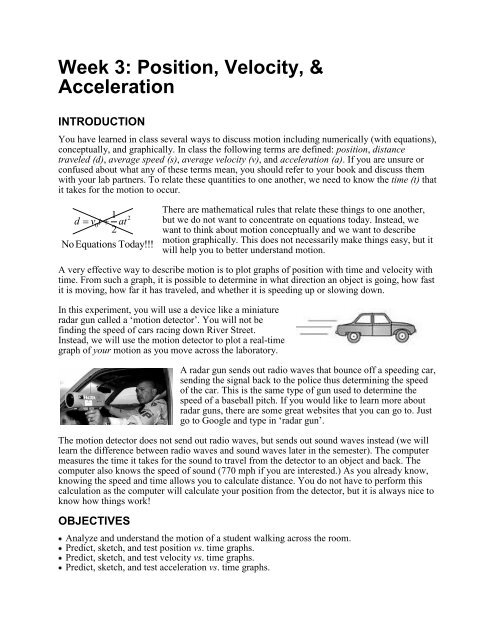
In this experiment, you will use a device like a miniature
radar gun called a „motion detector‟. You will not be
finding the speed of cars racing down River Street.
Instead, we will use the motion detector to plot a real-time
graph of your motion as you move across the laboratory.
A radar gun sends out radio waves that bounce off a speeding car,
sending the signal back to the police thus determining the speed
of the car. This is the same type of gun used to determine the
speed of a baseball pitch. If you would like to learn more about
radar guns, there are some great websites that you can go to. Just
go to Google and type in „radar gun‟.
The motion detector does not send out radio waves, but sends out sound waves instead (we will
learn the difference between radio waves and sound waves later in the semester). The computer
measures the time it takes for the sound to travel from the detector to an object and back. The
computer also knows the speed of sound (770 mph if you are interested.) As you already know,
knowing the speed and time allows you to calculate distance. You do not have to perform this
calculation as the computer will calculate your position from the detector, but it is always nice to
know how things work!
OBJECTIVES
Analyze and understand the motion of a student walking across the room.
Predict, sketch, and test position vs. time graphs.
Predict, sketch, and test velocity vs. time graphs.
Predict, sketch, and test acceleration vs. time graphs.

HINTS FOR EARNING A GOOD GRADE
It is very important that you THINK about what should happen before you perform an
experiment. This is true in lab, in class, and for all scientists in general.
You will be asked to predict what should happen using your knowledge of physics
You will then be asked to test your prediction.
If your prediction is proved to be correct, you may move on to the next question.
If your prediction is incorrect, your grade will not suffer, but you must explain why you
were wrong using your knowledge of physics.
If you take the time to predict correctly from the beginning, you will spend less time
overall on each question.
Use your knowledge of physics for all of your predictions and explanations!
Ask Questions!!!!
NECESSARY EQUIPMENT
Computer
Universal Lab Interface
Logger Pro
Vernier motion detector
meter stick
masking tape
PRELIMINARY STEPS
For experiments 1, 2 and 3 you need to do the following:
Connect the Motion Detector to PORT 2 of the Universal Lab Interface.
Place the Motion Detector so that it points toward an open space at least 4 m long. Use
short strips of masking tape on the floor to mark the 1 m, 2 m, 3 m, and 4 m distances from
the Motion Detector.
Prepare the computer for data collection: In Logger Pro, open the file "01a Graph
Matching" from the Physics with Vernier folder. A graph of position vs. time should
appear. Click on the Data menu and select "new column" then “formula.” Fill in the
following values: Name: acceleration, Short Name: Accel, Units: m/s^2, and Equation:
smooth secondDerivative("Position") Now click Done.
Test out the equipment! Using Logger Pro, produce a graph of your motion when you walk
away from the detector with constant velocity. To do this, stand about 1 m from the Motion
Detector and have your lab partner click Collect . Walk slowly away from the Motion
Detector when you hear it begin to click. Then walk toward the motion detector. There
should be a difference! You need to know why later. Play around a bit until you feel
comfortable, then move on to the experiment section below.

I. STANDING STILL
Standing still may not sound very exciting, but this is the simplest motion there is, so we will
start here.
You will need to sketch out several different graphs as predictions of
position vs. time. Though these are to be rough sketches, makes sure each
of your graphs have a horizontal axis (labeled time), a vertical axis
(labeled position), and an origin. (See picture to the right). You will also
have to sketch similar graphs of velocity vs. time.
1. Prediction: What should plots of position vs. time, velocity vs. time, and acceleration vs.
time look like for a person standing still? Sketch each out on a separate piece of paper
and remember to include some sort of explanation of why each looks the way it does.
2. Check Prediction: Now check your predictions. Using Logger Pro, produce position,
velocity, and acceleration vs. time graphs of your motion when you stand still. Now
sketch a copy of each next to the sketch you drew in your prediction. Do all agree? If not,
explain why your predictions were different.
II. CONSTANT VELOCITY
Moving at a constant velocity is a bit more exciting than standing still.
3. Prediction: What should plots of position vs. time, velocity vs. time, and acceleration vs.
time look like for a person moving at a constant speed? Sketch each out on a separate
piece of paper and remember to include some sort of explanation of why each looks the
way it does.
4. Check Prediction: Now check your predictions. Using Logger Pro, produce position,
velocity, and acceleration vs. time graphs of your motion when you move at a constant
speed toward the motion detector. Now sketch a copy of each next to the sketch you drew
in your prediction. Do all agree? If not, explain why your predictions were different.
III. ANALYSIS
5. In Logger Pro, determine the portion of the position vs. time graph in which you were
moving at constant velocity. Explain how you identified the time of constant velocity.
6. Highlight this portion of the graph. Under the “Analyze” menu, click “Linear Fit.” This
function determines the slope of a best-fit line through the highlighted data. Does a
straight line seem to fit the data?
7. What did Logger Pro calculate the slope of your position vs. time graph to be? Be sure to
include the units. The slope of any line is equal to the “rise” divided by the “run.” In this
case, the rise is distance, and the run is time. Using this idea, explain the units of the
slope.
8. What other quantity has these same units?

9. The fact that a straight line fit your position vs. time data indicates that the slope of your
graph is constant. Explain why this was to be expected, based on the manner in which
you were told to move.
10. Note the time at the beginning and ending of the highlighted section of the position vs.
time graph. Highlight this same section of time on the velocity vs. time graph. What
would you estimate that the average velocity is for this portion of the velocity vs. time
graph?
11. Under the “Analyze” menu, click “Statistics.” What did Logger Pro calculate as the
average, or “mean” value of velocity over this interval?
12. How does this value compare to the slope of the distance vs. time graph?
13. Compare these two values using a percent difference calculation.
IV: GRAPH MATCHING
Now that you are an expert on distance and velocity, you get to test your motion skills! First,
open "01b Graph Matching" from Logger Pro‟s Physics with Computes folder. The distance vs.
time graph shown below should appear.
14. Prediction: Describe, step by step, how you would walk to produce each of the five straight
segments on the graph above. Be sure to include a direction and time in each description.
15. What do you think your velocity will be for each segment? (Hint: Determine the slope of
each segment.)
16. Check Prediction: To test your prediction, choose a starting position and stand at that point.
Start data collection by clicking Collect . When you hear the Motion Detector begin to click,

walk in such a way that the graph of your motion matches the target graph on the computer
screen. This is not easy to do, and will probably require several trials to get a closely fitting
result.
17. Repeat: Every person in your group should repeat this process.
18. Analysis: When the last person in the group has created a good match, perform an analysis
on the data. Highlight each segment individually, and determine and record each velocity
using the linear fit function.
19. Using percent difference, compare the valued Logger Pro calculated as the velocity of the
second segment to your predicted value.