Optimizing Location, Routing and Scheduling Decisions ... - gerad
Optimizing Location, Routing and Scheduling Decisions ... - gerad
Optimizing Location, Routing and Scheduling Decisions ... - gerad

You also want an ePaper? Increase the reach of your titles
YUMPU automatically turns print PDFs into web optimized ePapers that Google loves.
Introduction<br />
Problem Definition <strong>and</strong> Formulation<br />
Solution Methodology<br />
Conclusion<br />
References<br />
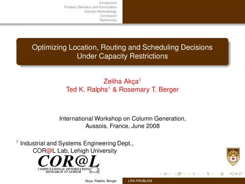
<strong>Optimizing</strong> <strong>Location</strong>, <strong>Routing</strong> <strong>and</strong> <strong>Scheduling</strong> <strong>Decisions</strong><br />
Under Capacity Restrictions<br />
Zeliha Akça 1<br />
Ted K. Ralphs 1 & Rosemary T. Berger<br />
International Workshop on Column Generation,<br />
Aussois, France, June 2008<br />
1 Industrial <strong>and</strong> Systems Engineering Dept.,<br />
COR@L Lab, Lehigh University<br />
Akça, Ralphs, Berger<br />
LRS PROBLEM
Outline<br />
Introduction<br />
Problem Definition <strong>and</strong> Formulation<br />
Solution Methodology<br />
Conclusion<br />
References<br />
1 Introduction<br />
2 Problem Definition <strong>and</strong> Formulation<br />
Problem Definition<br />
Set Partitioning Formulation<br />
3 Solution Methodology<br />
Pricing Problem<br />
Branching<br />
Improving Branch <strong>and</strong> Price Algorithm<br />
Computational Results<br />
4 Conclusion<br />
Akça, Ralphs, Berger<br />
LRS PROBLEM
Introduction<br />
Problem Definition <strong>and</strong> Formulation<br />
Solution Methodology<br />
Conclusion<br />
References<br />
<strong>Location</strong> <strong>Routing</strong> & <strong>Scheduling</strong> (LRS) Problem<br />
LRS problem integrates the decisions of determining<br />
the optimal number <strong>and</strong> locations of facilities,<br />
an optimal set of vehicle routes from facilities to customers<br />
an optimal assignment of routes to vehicles subject to scheduling<br />
constraints.<br />
The objective is to minimize the total fixed costs <strong>and</strong> operating costs of<br />
facilities <strong>and</strong> vehicles.<br />
Vehicle 1<br />
Vehicle 2<br />
Vehicle 3<br />
Vehicle 4<br />
Customer<br />
Facility<br />
Akça, Ralphs, Berger<br />
LRS PROBLEM
Motivation<br />
Introduction<br />
Problem Definition <strong>and</strong> Formulation<br />
Solution Methodology<br />
Conclusion<br />
References<br />
For multiple customer routes, location <strong>and</strong> routing are interdependent.<br />
One-to-one relationship between vehicles <strong>and</strong> routes overestimates the<br />
number of vehicles used <strong>and</strong> costs.<br />
Large fixed costs for vehicles <strong>and</strong> drivers.<br />
Constant fleet size.<br />
Working hour limit for drivers.<br />
Time sensitive items.<br />
Akça, Ralphs, Berger<br />
LRS PROBLEM
Introduction<br />
Problem Definition <strong>and</strong> Formulation<br />
Solution Methodology<br />
Conclusion<br />
References<br />
LRSP in Literature<br />
Lin et al. [2002]:<br />
Introduce the problem for a phone company.<br />
Divide the problem into 3 phases: facility location, vehicle routing <strong>and</strong><br />
loading.<br />
Construct a heuristic algorithm which includes some metaheuristics.<br />
Solve a real instance with 27 customers <strong>and</strong> 4 c<strong>and</strong>idate facilities.<br />
Lin <strong>and</strong> Kwok [2005]:<br />
Extend the study to a multi-objective LRS problem.<br />
They develop a similar heuristic algorithm.<br />
Real instances with 27 customers <strong>and</strong> 85 customers,<br />
R<strong>and</strong>om instances up to 200 customers.<br />
Akça, Ralphs, Berger<br />
LRS PROBLEM
Problem Definition<br />
Introduction<br />
Problem Definition <strong>and</strong> Formulation<br />
Solution Methodology<br />
Conclusion<br />
References<br />
Problem Definition<br />
Set Partitioning Formulation<br />
Objective<br />
to select a subset of the facilities, construct a set of delivery routes <strong>and</strong> to<br />
assign routes to vehicles with minimum total cost.<br />
Constraints<br />
Capacitated facilities.<br />
Capacitated vehicles.<br />
Time limit for the vehicles.<br />
Each customer must be visited exactly once.<br />
Each route <strong>and</strong> vehicle must start at a facility <strong>and</strong> return to the same<br />
facility.<br />
Akça, Ralphs, Berger<br />
LRS PROBLEM
Pairing Concept<br />
Introduction<br />
Problem Definition <strong>and</strong> Formulation<br />
Solution Methodology<br />
Conclusion<br />
References<br />
Problem Definition<br />
Set Partitioning Formulation<br />
Pairing:<br />
A set of routes that can be served sequentially by one vehicle within the<br />
vehicle’s working hour limit.<br />
PAIRING<br />
FACILITY<br />
CUSTOMER<br />
A pairing is feasible if<br />
each customer included in the pairing<br />
is visited once,<br />
each route included starts <strong>and</strong> ends<br />
at the same facility,<br />
total dem<strong>and</strong> of each route ≤ vehicle<br />
capacity,<br />
total travel time of the pairing ≤<br />
vehicle working hour limit<br />
PAIRING<br />
Akça, Ralphs, Berger<br />
LRS PROBLEM
Introduction<br />
Problem Definition <strong>and</strong> Formulation<br />
Solution Methodology<br />
Conclusion<br />
References<br />
Set Partitioning-based model: Notation<br />
Problem Definition<br />
Set Partitioning Formulation<br />
Sets<br />
I = set of dem<strong>and</strong> nodes<br />
J = set of c<strong>and</strong>idate facility locations<br />
P j = set of all feasible pairings for facility j, ∀j ∈ J<br />
Parameters<br />
j 1 if dem<strong>and</strong> node i is in pairing p of facility j, ∀i ∈ I, j ∈ J, p ∈ Pj<br />
a ip =<br />
0 otherwise<br />
C p = cost of pairing p associated with facility j, ∀p ∈ P j, j ∈ J<br />
F j = fixed cost of opening facility j, ∀j ∈ J<br />
C F j = capacity of facility j, ∀j ∈ J<br />
Decision Variables<br />
j 1 if pairing p is selected for facility j, ∀p ∈ Pj <strong>and</strong> j ∈ J<br />
z p =<br />
0 otherwise<br />
j 1 if facility j is selected, ∀j ∈ J<br />
t j =<br />
0 otherwise<br />
Akça, Ralphs, Berger<br />
LRS PROBLEM
Introduction<br />
Problem Definition <strong>and</strong> Formulation<br />
Solution Methodology<br />
Conclusion<br />
References<br />
Set Partitioning Formulation<br />
Problem Definition<br />
Set Partitioning Formulation<br />
(SPP-LRS)<br />
Minimize<br />
subject to<br />
X j∈J<br />
F jt j + X X<br />
C pz p (1)<br />
j∈J p∈P j<br />
X X<br />
a ipz p = 1 ∀i ∈ I (π i ), (2)<br />
j∈J p∈P j<br />
X<br />
a ipD iz p ≤ Cj F t j ∀j ∈ J (µ j ), (3)<br />
X<br />
p∈P j i∈I<br />
z p ∈ {0, 1} ∀p ∈ P j, ∀j ∈ J, (4)<br />
t j ∈ {0, 1} ∀j ∈ J. (5)<br />
Akça, Ralphs, Berger<br />
LRS PROBLEM
Simple Valid Inequalities<br />
Introduction<br />
Problem Definition <strong>and</strong> Formulation<br />
Solution Methodology<br />
Conclusion<br />
References<br />
Problem Definition<br />
Set Partitioning Formulation<br />
X<br />
a ipz p ≤ t j ∀i ∈ I, ∀j ∈ J (σ ji ), (6)<br />
p∈P j<br />
X<br />
t j ≥ N F , (7)<br />
j∈J<br />
X<br />
z p = v j ∀j ∈ J (ν j ), (8)<br />
p∈P j<br />
v j ≥ t j ∀j ∈ J, (9)<br />
v j ∈ Z + ∀j ∈ J. (10)<br />
N F is the minimum number of facilities required to be open:<br />
N F = argmin {l=1..|J|}<br />
lX<br />
Cj F t<br />
≥ X !<br />
D i<br />
t=1 i∈I<br />
s.t. Cj F 1<br />
≥ Cj F 2<br />
≥ ... ≥ Cj F n<br />
Akça, Ralphs, Berger<br />
LRS PROBLEM
Introduction<br />
Problem Definition <strong>and</strong> Formulation<br />
Solution Methodology<br />
Conclusion<br />
References<br />
Branch <strong>and</strong> Price Algorithm<br />
Pricing Problem<br />
Branching<br />
Improving Branch <strong>and</strong> Price Algorithm<br />
Computational Results<br />
Initial Columns<br />
Solve<br />
Restricted Master Problem<br />
(RMP)<br />
Dual Variables<br />
Until no<br />
new column<br />
new columns<br />
Optimal Soln. of RMP=LOWER BD<br />
IP Soln. of RMP=UPPER BD.<br />
Solve<br />
Pricing Problem:<br />
Find columns<br />
with (−) reduced<br />
cost<br />
ROOT NODE<br />
If LP is not integral<br />
Branching<br />
MODIFIED RPM<br />
Constraints + Variable Fixing<br />
MODIFIED RPM<br />
Constraints + Variable Fixing<br />
Solve LP<br />
Solve<br />
MODIFIED<br />
Pricing Problem<br />
Solve LP<br />
Solve<br />
MODIFIED<br />
Pricing Problem<br />
Akça, Ralphs, Berger<br />
LRS PROBLEM
Introduction<br />
Problem Definition <strong>and</strong> Formulation<br />
Solution Methodology<br />
Conclusion<br />
References<br />
Describing Pricing Problem<br />
Pricing Problem<br />
Branching<br />
Improving Branch <strong>and</strong> Price Algorithm<br />
Computational Results<br />
Objective<br />
To find a pairing (a set of routes) associated with a variable with minimum<br />
reduced cost:<br />
Ĉ p = C p − X a ip · π i + X a ip · d i · µ j + X a ip · σ ji − ν j ∀p ∈ P j, j ∈ J (11)<br />
i∈N<br />
i∈N<br />
i∈N<br />
Subject to<br />
All of the routes must start & end at the same facility.<br />
Each customer node can be visited at most once.<br />
Total dem<strong>and</strong> of each route ≤ vehicle capacity.<br />
Total travel time of the pairing ≤ time limit.<br />
Akça, Ralphs, Berger<br />
LRS PROBLEM
Introduction<br />
Problem Definition <strong>and</strong> Formulation<br />
Solution Methodology<br />
Conclusion<br />
References<br />
Pricing Problem as a Network Problem: Cont.<br />
Pricing Problem<br />
Branching<br />
Improving Branch <strong>and</strong> Price Algorithm<br />
Computational Results<br />
For each facility, construct a network with source <strong>and</strong> sink.<br />
d1<br />
1<br />
2<br />
d2<br />
0<br />
Source<br />
Facility j<br />
−VCap<br />
Sink<br />
Facility j<br />
Cost of arc (i, k) in network for facility j:<br />
d3<br />
3<br />
ĉ ik =<br />
j<br />
cik − π k + d kµ j + σ jk<br />
c ik<br />
if k is a customer node<br />
otherwise<br />
Elementary (wrt. customer nodes), resource constraint shortest path<br />
problem (ESPPRC).<br />
Not elementary wrt sink → multiple vehicle routes.<br />
Sink is the end of a route <strong>and</strong> possibly beginning of another one.<br />
Akça, Ralphs, Berger<br />
LRS PROBLEM
Solving Pricing Problem<br />
Introduction<br />
Problem Definition <strong>and</strong> Formulation<br />
Solution Methodology<br />
Conclusion<br />
References<br />
Pricing Problem<br />
Branching<br />
Improving Branch <strong>and</strong> Price Algorithm<br />
Computational Results<br />
Label setting algorithm by Feillet et al. [2004] to solve ESPPRC.<br />
All possible paths from source to sink are assigned a label.<br />
To reduce the number of labels, only the labels that are not dominated<br />
by any other label are considered.<br />
2-phase ESPPRC Algorithm to Find Pairings<br />
Phase 1: Network includes a source, a sink <strong>and</strong> customer nodes.<br />
Run ESPPRC algorithm with vehicle capacity <strong>and</strong> time limit resources.<br />
Run domination algorithm for the labels of sink.<br />
Phase 2: Network includes a source, a sink <strong>and</strong> sink labels from phase 1.<br />
Each node starts with the label from Phase 1.<br />
Run ESPPRC algorithm with time limit resource.<br />
Akça, Ralphs, Berger<br />
LRS PROBLEM
Branching Rules<br />
Introduction<br />
Problem Definition <strong>and</strong> Formulation<br />
Solution Methodology<br />
Conclusion<br />
References<br />
Pricing Problem<br />
Branching<br />
Improving Branch <strong>and</strong> Price Algorithm<br />
Computational Results<br />
Rule 1 Facility location variables → OPEN \ CLOSED.<br />
Simple, no need to update the pricing problems.<br />
Rule 2 Total # of vehicles at each facility → INTEGER<br />
Just a fixed cost change in the total reduced cost of a column.<br />
Rule 3 A customer can only be assigned to 1 facility<br />
→ FORCE customer i must be served by facility j:<br />
X<br />
p∈P j<br />
a ipZ p ≥ 1 (γ ji) (12)<br />
→ FORBID customer i cannot be served by facility j:<br />
X<br />
Easy to incorporate into pricing problem.<br />
Rule 4 Branching on flow on single arcs.<br />
p∈P j<br />
a ipZ p ≤ 0 (13)<br />
Akça, Ralphs, Berger<br />
LRS PROBLEM
Introduction<br />
Problem Definition <strong>and</strong> Formulation<br />
Solution Methodology<br />
Conclusion<br />
References<br />
Heuristic Solutions For Pricing Problem<br />
Pricing Problem<br />
Branching<br />
Improving Branch <strong>and</strong> Price Algorithm<br />
Computational Results<br />
ESPPRC with Label Limit (ESPPRC - LL(n))<br />
Set a label limit, n.<br />
Sort the labels of node on reduced cost.<br />
Keep at most n of the non processed labels with smallest reduced cost.<br />
For small values of n, it is very quick.<br />
Label limit can be gradually increased.<br />
ESPPRC for a Subset of Customers (ESPPRC - CS(n))<br />
Choose n based on the average dem<strong>and</strong> <strong>and</strong> vehicle capacity.<br />
Choose a subset of customers C S with size n based on reduced costs of<br />
arcs in the network.<br />
Apply ESPPRC algorithm to customer set C S.<br />
Akça, Ralphs, Berger<br />
LRS PROBLEM
Introduction<br />
Problem Definition <strong>and</strong> Formulation<br />
Solution Methodology<br />
Conclusion<br />
References<br />
2-Step Branch & Price Algorithm<br />
Pricing Problem<br />
Branching<br />
Improving Branch <strong>and</strong> Price Algorithm<br />
Computational Results<br />
STEP 1: Heuristic Branch <strong>and</strong> Price Tree<br />
Initial Column<br />
Generator<br />
Heuristic<br />
Upper Bound<br />
Branching<br />
Rules<br />
BP Tree<br />
ESPPRC − LL(n)<br />
+<br />
ESPPRC −CS(m)<br />
STEP 2: Exact Branch <strong>and</strong> Price Tree<br />
Columns + Upper Bound<br />
from STEP 1<br />
Branching<br />
Rules<br />
BP Tree<br />
ESPPRC − LL(n)<br />
+<br />
ESPPRC −CS(m)<br />
+<br />
Exact Pricing Problem<br />
Akça, Ralphs, Berger<br />
LRS PROBLEM
Introduction<br />
Problem Definition <strong>and</strong> Formulation<br />
Solution Methodology<br />
Conclusion<br />
References<br />
Implementation <strong>and</strong> Test Problems<br />
Pricing Problem<br />
Branching<br />
Improving Branch <strong>and</strong> Price Algorithm<br />
Computational Results<br />
MINTO 3.1 <strong>and</strong> CPLEX 9.1.<br />
Customer <strong>and</strong> c<strong>and</strong>idate facility locations, customer dem<strong>and</strong>s are<br />
generated using MDVRP benchmark problems developed by Cordeau<br />
et al. [1995].<br />
Instances with 25 <strong>and</strong> 40 customers <strong>and</strong> 5 facilities.<br />
For each set of locations, 2 possible vehicle capacity, 2 possible time<br />
limit values are used.<br />
For 25 customer instances, 1 step branch & price (8 CPU hours).<br />
For 40 customer instances, 2 step branch & price: Step 1 (Heuristic BP)<br />
is run for 2 CPU hours.<br />
Step 2 of the algorithm (Exact BP) is run for 6 CPU hours.<br />
Akça, Ralphs, Berger<br />
LRS PROBLEM
Introduction<br />
Problem Definition <strong>and</strong> Formulation<br />
Solution Methodology<br />
Conclusion<br />
References<br />
Effect of ESPPRC - CS(n)<br />
Pricing Problem<br />
Branching<br />
Improving Branch <strong>and</strong> Price Algorithm<br />
Computational Results<br />
Data With out SS With SS Data With out SS With SS<br />
UB-S1 Gap-S2 UB-S1 Gap-S2 UB-S1 Gap-S2 UB-S1 Gap-S2<br />
a40-v1t1 7131 0.01% 7131 0 e40-v1t1 7167 0 7167 0<br />
a40-v1t2 6986 0.14% 7170 0.32% e40-v1t2 6950 0.07% 6950 0.05%<br />
a40-v2t1 7017 0 6866 0 e40-v2t1 6857 0 6849 0<br />
a40-v2t2 6821 1.99% 6821 1.26% e40-v2t2 6846 3.19% 6846 0<br />
b40-v1t1 7252 4.14% 7183 3.22% f40-v1t1 7167 0 7167 0<br />
b40-v1t2 6934 0 6934 0 f40-v1t2 7001 0 7001 0<br />
b40-v2t1 6823 0 6823 0 f40-v2t1 6925 0.01% 6881 0<br />
b40-v2t2 6634 0 6633 0 f40-v2t2 6851 2.55% 6845 2.34%<br />
c40-v1t1 8780 0 8780 0 g40-v1t1 7343 0 7343 0<br />
c40-v1t2 8756 0 8753 0 g40-v1t2 7117 0 7124 0<br />
c40-v2t1 8663 0 8663 0 g40-v2t1 7000 0 7005 0<br />
c40-v2t2 8456 0 8438 0 g40-v2t2 6944 0 6944 0<br />
d40-v1t1 7793 0.23% 7740 0 h40-v1t1 7012 0.01% 7013 0<br />
d40-v1t2 7544 6.32% 7236 2.95% h40-v1t2 6972 1.22% 6972 0.35%<br />
d40-v2t1 7140 2.29% 7132 2.79% h40-v2t1 6869 3.01% 6857 0.04%<br />
d40-v2t2 7430 8.52% 6947 4.18% h40-v2t2 6667 1.78% 6658 1.64%<br />
Step 1 time → 3.4, step 2 time → 1.57, <strong>and</strong> total time → 1.61.<br />
Akça, Ralphs, Berger<br />
LRS PROBLEM
Introduction<br />
Problem Definition <strong>and</strong> Formulation<br />
Solution Methodology<br />
Conclusion<br />
References<br />
Pricing Problem<br />
Branching<br />
Improving Branch <strong>and</strong> Price Algorithm<br />
Computational Results<br />
1 Step Branch & Price Algorithm for 25 Customer Instances<br />
Akça, Ralphs, Berger<br />
LRS PROBLEM
Introduction<br />
Problem Definition <strong>and</strong> Formulation<br />
Solution Methodology<br />
Conclusion<br />
References<br />
Pricing Problem<br />
Branching<br />
Improving Branch <strong>and</strong> Price Algorithm<br />
Computational Results<br />
2 Step Branch & Price Algorithm for 40 Customer Instances<br />
Akça, Ralphs, Berger<br />
LRS PROBLEM
Introduction<br />
Problem Definition <strong>and</strong> Formulation<br />
Solution Methodology<br />
Conclusion<br />
References<br />
Pricing Problem<br />
Branching<br />
Improving Branch <strong>and</strong> Price Algorithm<br />
Computational Results<br />
Comparison with Literature: Lin et. al (2002) Instances<br />
Instances Branch & Bound Best Heuristic<br />
Obj. CPU (s) Obj. CPU (s)<br />
1: 4 depots, 10 custs. 309,817 1155 309,817 0.44<br />
2: 4 depots, 10 custs. 309,808 982 309,808 0.49<br />
3: 4 depots, 12 custs. 312,036* > 10,000 312,036 0.82<br />
4: 4 depots, 27 custs. - - 625,752.5 6<br />
* Best solution in 10000 CPU seconds in a Pentium III machine.<br />
a. Lin et. al (2002)<br />
Instances Obj. CPU (s)<br />
1: 4 depots, 10 custs. 309,817 0.70<br />
2: 4 depots, 10 custs. 309,808 0.26<br />
3: 4 depots, 12 custs. 312,036 0.13<br />
4: 4 depots, 27 custs. 625,750.167 135.20<br />
b. 1 Step Branch <strong>and</strong> Price Algorithm<br />
Akça, Ralphs, Berger<br />
LRS PROBLEM
Introduction<br />
Problem Definition <strong>and</strong> Formulation<br />
Solution Methodology<br />
Conclusion<br />
References<br />
Pricing Problem<br />
Branching<br />
Improving Branch <strong>and</strong> Price Algorithm<br />
Computational Results<br />
Effect of <strong>Scheduling</strong> Constraint: LRSP vs LRP-DC<br />
One of the open facilities is different in 3 of the instances.<br />
Akça, Ralphs, Berger<br />
LRS PROBLEM
Introduction<br />
Problem Definition <strong>and</strong> Formulation<br />
Solution Methodology<br />
Conclusion<br />
References<br />
Pricing Problem<br />
Branching<br />
Improving Branch <strong>and</strong> Price Algorithm<br />
Computational Results<br />
Effect of <strong>Scheduling</strong> Constraint: LRSP vs LRP-DC<br />
Akça, Ralphs, Berger<br />
LRS PROBLEM
Conclusions<br />
Introduction<br />
Problem Definition <strong>and</strong> Formulation<br />
Solution Methodology<br />
Conclusion<br />
References<br />
Formulated <strong>and</strong> designed a branch <strong>and</strong> price algorithm to solve the<br />
LRSP to optimally.<br />
Enhanced the algorithm by a heuristic pricing problems <strong>and</strong> by a<br />
heuristic step.<br />
Solved instances up to 40 customers <strong>and</strong> 5 facilities.<br />
Solved LRP-DC <strong>and</strong> ompare the costs with LRSP.<br />
Akça, Ralphs, Berger<br />
LRS PROBLEM
Introduction<br />
Problem Definition <strong>and</strong> Formulation<br />
Solution Methodology<br />
Conclusion<br />
References<br />
J.F. Cordeau, M. Gendreau, <strong>and</strong> G. Laporte. A Tabu Search Heuristic for<br />
Periodic <strong>and</strong> Multi-Depot Vehicle <strong>Routing</strong> Problems, 1995. Technical<br />
Report 95-75, Center for Research on Transportation, Montréal. Available<br />
at neo.lcc.uma.es/radiaeb/WebVRP/Problem<br />
Instances/CordeauFilesDesc.html.<br />
D. Feillet, P. Dejax, M. Gendreau, <strong>and</strong> C. Gueguen. An Exact Algorithm for<br />
the Elementary Shortest Path Problem with Resource Constraints:<br />
Application to Some Vehicle <strong>Routing</strong> Problems. Networks, 44(3):216–229,<br />
2004.<br />
C.K. Lin, C.K. Chew, <strong>and</strong> A. Chen. A <strong>Location</strong>-<strong>Routing</strong>-Loading Problem for<br />
Bill Delivery Services. Computers <strong>and</strong> Industrial Engineering, 43:5–25,<br />
2002.<br />
C.K. Lin <strong>and</strong> R.C.W. Kwok. Multi-Objective Metaheuristics for a<br />
<strong>Location</strong>-<strong>Routing</strong> Problem withMultiple Use of Vehicles on Real Data <strong>and</strong><br />
Simulated Date. European Journal of Operational Research, In Press,<br />
2005.<br />
Akça, Ralphs, Berger<br />
LRS PROBLEM