Manifold Alignment without Correspondence - University of ...

defined by different features for different tasks and it is hard
to find correspondences between them. This problem can be
more precisely defined as follows: suppose we have two data
sets X = {x 1 , · · · , x m } and Y = {y 1 , · · · , y n } for which
we want to find correspondence, our aim is to compute functions
α and β to map x i and y j to the same space such that
α T x i and β T y j can be directly compared.
To solve the problem mentioned above, the new algorithm
(illustrated in Figure 1(C)) needs to go beyond the regular
manifold alignment in that it should be able to map the data
instances (from two different spaces) to a new lower dimensional
space without using correspondence information. We
also want the resulting alignment to be defined everywhere
rather than just on the training instances, so that it can handle
new test points. In this paper, we propose a novel approach
to learn such mapping functions α and β to project
the data instances to a new lower dimensional space by simultaneously
matching the local geometry and preserving the
neighborhood relationship within each set. In addition to the
theoretical analysis of our algorithm, we also report on several
real-world applications of the new alignment approach
in information retrieval and bioinformatics. Notation used in
this paper is defined and explained in Figure 3.
The rest of this paper is as follows. In Section 2 we describe
the main algorithm. In Section 3 we explain the rationality
underlying our approach. We describe some novel applications
and summarize experimental results in Section 4.
Section 5 provides some concluding remarks.
2 The Main Algorithm
2.1 The Problem
As defined in Figure 3, X is a set of samples collected from
manifold X ; Y is a set of samples collected from manifold
Y. We want to learn mappings α and β to map X and Y to a
new space Z, where the neighborhood relationships inside of
X and Y will be preserved, and if local geometries of x i and
y j are matched in the original spaces, they will be neighbors
in the new space.
2.2 High Level Explanation
The data sets X and Y are represented by different features.
Thus, it is difficult to directly compare x i and y j . To build
connections between them, we use the relation between x i
and its neighbors to characterize x i ’s local geometry. Using
relations rather than features to represent local geometry
makes the direct comparison of x i and y j be possible. However,
x i might be similar to more than one instance in Y , and
it is hard to identify which one is the true match (in fact, for
many applications, there is more than one true match).
An interesting fact is that solving the original coupled
problem could be easier than only finding the true match. The
reason is the structure of both manifolds need to be preserved
in the alignment. This helps us get rid of many false positive
matches. In our algorithm, we first identify all the possible
matches for each instance leveraging its local geometry. Then
we convert the alignment problem to an embedding problem
with constraints. The latter can be solved by solving a generalized
eigenvalue decomposition problem.
x©
y
X
Y
x©
y
x©
Figure 2: Illustration of the main algorithm.
2.3 The Algorithm
Assume the kernels for computing the similarity between data
points in each of the two data sets are already given (for example,
heat kernel). The algorithm is as follows:
1. Create connections between local geometries:
• W ij = e −dist(Rx i ,Ry j )/δ2 , where R xi , R yj ,
and W are defined and explained in Figure 3,
dist(R xi , R yj ) is defined in Sec 3.2.
• The definition of W ij could be application oriented.
Using other ways to define W ij does not
affect the other parts of the algorithm.
2. Join the two manifolds:
• Compute the matrices L, Z and D, which are used
to model the joint structure.
3. Compute the optimal projection to reduce the dimensionality
of the joint structure:
• The d dimensional projection is computed by d
minimum eigenvectors γ 1 · · · γ d of the generalized
eigenvalue decomposition ZLZ T γ = λZDZ T γ.
4. Find the correspondence between X and Y :
• Let A be the top p rows of [γ 1 · · · γ d ], and B be
the next q rows. For any i and j, A T x i and B T y j
are in the same space and can be directly compared.
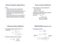
The algorithm is illustrated in Figure 2. x i ∈ X and
y j ∈ Y are from different manifolds, so they cannot be directly
compared. Our algorithm learns a mapping A for X
and a mapping B for Y to map the two manifolds to one
space so that instances (from different manifolds) with similar
local geometry will be mapped to similar locations and
the manifold structures will also be preserved. Computing A
and B is tricky. Steps 1 and 2 are in fact joining the two manifolds
so that their underlying structures in common can be
explored. Step 3 computes a mapping to( map the ) joint structure
to a lower dimensional space, where = [γ A
B
1 · · · γ d ]
is used for manifold alignment. Section 3 explains the rationale
underlying the approach. Once A and B are available
to us, AB + and BA + can be used as “keys” to translate instances
between spaces defined by totally different features
(for example, one is in English, another is in Chinese). The
algorithm can also be used when partial correspondence information
is available (see Sec 4.2 for more details).
y