Manifold Alignment without Correspondence - University of ...

¡
¢
Manifold Alignment without Correspondence
Chang Wang and Sridhar Mahadevan
Computer Science Department
University of Massachusetts
Amherst, Massachusetts 01003
{chwang, mahadeva}@cs.umass.edu
Abstract
Manifold alignment has been found to be useful
in many areas of machine learning and data mining.
In this paper we introduce a novel manifold
alignment approach, which differs from “semisupervised
alignment” and “Procrustes alignment”
in that it does not require predetermining correspondences.
Our approach learns a projection that
maps data instances (from two different spaces) to
a lower dimensional space simultaneously matching
the local geometry and preserving the neighborhood
relationship within each set. This approach
also builds connections between spaces defined
by different features and makes direct knowledge
transfer possible. The performance of our algorithm
is demonstrated and validated in a series of
carefully designed experiments in information retrieval
and bioinformatics.
1 Introduction
In many areas of machine learning and data mining, one is
often confronted with situations where the data is in a high
dimensional space. Directly dealing with such high dimensional
data is usually intractable, but in many cases, the underlying
manifold structure may have a low intrinsic dimensionality.
Manifold alignment builds connections between
two or more disparate data sets by aligning their underlying
manifolds and provides knowledge transfer across the
data sets. Real-world applications include automatic machine
translation [Diaz & Metzler, 2007], representation and
control transfer in Markov decision processes, bioinformatics
[Wang & Mahadevan, 2008], and image interpretation.
Two previously studied manifold alignment approaches are
Procrustes alignment [Wang & Mahadevan, 2008] and semisupervised
alignment [Ham et al., 2005].
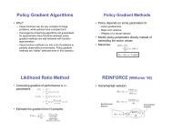
Procrustes alignment (illustrated in Figure 1(A)) is a two
step algorithm leveraging pairwise correspondences between
a subset of the instances. In the first step, the entire data
sets are mapped to low dimensional spaces reflecting their
intrinsic geometries using a standard (linear like LPP [He &
Niyogi, 2003] or nonlinear like Laplacian eigenmaps [Belkin
& Niyogi, 2003]) dimensionality reduction approach. In the
£ ¤¦¥¨§
¡
¡
( A ) ( B ) ( C )
Figure 1: Comparison of different manifold alignment approaches.
X and Y are the spaces where manifolds are defined
on. Z is the new lower dimensional space. The red
regions represent the subsets that are in correspondence. (A)
Procrustes manifold alignment; (B) Semi-supervised manifold
alignment; (C) The new approach: α and β are mapping
functions.
second step, the translational, rotational and scaling components
are removed from one set so that the optimal alignment
between the instances in correspondence is achieved.
Procrustes alignment learns a mapping defined everywhere,
when a suitable dimensionality reduction method is used, so
it can handle the new test points. In Procrustes alignment, the
computation of lower dimensional embeddings is done in a
unsupervised way (without considering the purpose of alignment),
so the resulting embeddings of the two data sets might
be quite different. Semi-supervised alignment (illustrated in
Figure 1(B)) also uses a set of correspondences to align the
manifolds. In this approach, the points of the two data sets
are mapped to a new space by solving a constrained embedding
problem, where the embeddings of the corresponding
points from different sets are constrained to be close to each
other. A significant disadvantage of this approach is that it
directly computes the embedding results rather than the mapping
functions, so the alignment is defined only on the known
data points, and it is hard to handle the new test points.
A more general manifold alignment problem arises in
many real world applications, where two manifolds (defined
by totally different features) need to be aligned with no correspondence
information available to us. Solving this problem
is rather difficult, if not impossible, since there are two unknown
variables in this problem: the correspondence and the
transformation. One such example is control transfer between
different Markov decision processes (MDPs), where we want
to align state spaces of different tasks. Here, states are usually

defined by different features for different tasks and it is hard
to find correspondences between them. This problem can be
more precisely defined as follows: suppose we have two data
sets X = {x 1 , · · · , x m } and Y = {y 1 , · · · , y n } for which
we want to find correspondence, our aim is to compute functions
α and β to map x i and y j to the same space such that
α T x i and β T y j can be directly compared.
To solve the problem mentioned above, the new algorithm
(illustrated in Figure 1(C)) needs to go beyond the regular
manifold alignment in that it should be able to map the data
instances (from two different spaces) to a new lower dimensional
space without using correspondence information. We
also want the resulting alignment to be defined everywhere
rather than just on the training instances, so that it can handle
new test points. In this paper, we propose a novel approach
to learn such mapping functions α and β to project
the data instances to a new lower dimensional space by simultaneously
matching the local geometry and preserving the
neighborhood relationship within each set. In addition to the
theoretical analysis of our algorithm, we also report on several
real-world applications of the new alignment approach
in information retrieval and bioinformatics. Notation used in
this paper is defined and explained in Figure 3.
The rest of this paper is as follows. In Section 2 we describe
the main algorithm. In Section 3 we explain the rationality
underlying our approach. We describe some novel applications
and summarize experimental results in Section 4.
Section 5 provides some concluding remarks.
2 The Main Algorithm
2.1 The Problem
As defined in Figure 3, X is a set of samples collected from
manifold X ; Y is a set of samples collected from manifold
Y. We want to learn mappings α and β to map X and Y to a
new space Z, where the neighborhood relationships inside of
X and Y will be preserved, and if local geometries of x i and
y j are matched in the original spaces, they will be neighbors
in the new space.
2.2 High Level Explanation
The data sets X and Y are represented by different features.
Thus, it is difficult to directly compare x i and y j . To build
connections between them, we use the relation between x i
and its neighbors to characterize x i ’s local geometry. Using
relations rather than features to represent local geometry
makes the direct comparison of x i and y j be possible. However,
x i might be similar to more than one instance in Y , and
it is hard to identify which one is the true match (in fact, for
many applications, there is more than one true match).
An interesting fact is that solving the original coupled
problem could be easier than only finding the true match. The
reason is the structure of both manifolds need to be preserved
in the alignment. This helps us get rid of many false positive
matches. In our algorithm, we first identify all the possible
matches for each instance leveraging its local geometry. Then
we convert the alignment problem to an embedding problem
with constraints. The latter can be solved by solving a generalized
eigenvalue decomposition problem.
x©
y
X
Y
x©
y
x©
Figure 2: Illustration of the main algorithm.
2.3 The Algorithm
Assume the kernels for computing the similarity between data
points in each of the two data sets are already given (for example,
heat kernel). The algorithm is as follows:
1. Create connections between local geometries:
• W ij = e −dist(Rx i ,Ry j )/δ2 , where R xi , R yj ,
and W are defined and explained in Figure 3,
dist(R xi , R yj ) is defined in Sec 3.2.
• The definition of W ij could be application oriented.
Using other ways to define W ij does not
affect the other parts of the algorithm.
2. Join the two manifolds:
• Compute the matrices L, Z and D, which are used
to model the joint structure.
3. Compute the optimal projection to reduce the dimensionality
of the joint structure:
• The d dimensional projection is computed by d
minimum eigenvectors γ 1 · · · γ d of the generalized
eigenvalue decomposition ZLZ T γ = λZDZ T γ.
4. Find the correspondence between X and Y :
• Let A be the top p rows of [γ 1 · · · γ d ], and B be
the next q rows. For any i and j, A T x i and B T y j
are in the same space and can be directly compared.
The algorithm is illustrated in Figure 2. x i ∈ X and
y j ∈ Y are from different manifolds, so they cannot be directly
compared. Our algorithm learns a mapping A for X
and a mapping B for Y to map the two manifolds to one
space so that instances (from different manifolds) with similar
local geometry will be mapped to similar locations and
the manifold structures will also be preserved. Computing A
and B is tricky. Steps 1 and 2 are in fact joining the two manifolds
so that their underlying structures in common can be
explored. Step 3 computes a mapping to( map the ) joint structure
to a lower dimensional space, where = [γ A
B
1 · · · γ d ]
is used for manifold alignment. Section 3 explains the rationale
underlying the approach. Once A and B are available
to us, AB + and BA + can be used as “keys” to translate instances
between spaces defined by totally different features
(for example, one is in English, another is in Chinese). The
algorithm can also be used when partial correspondence information
is available (see Sec 4.2 for more details).
y

x i is defined in a p dimensional space (manifold X ), and
the p features are {f 1 , · · · , f p };
X = {x 1 , · · · , x m }, X is a p × m matrix.
Wx
i,j is the similarity of x i and x j (could be defined by
heat kernel).
D x is a diagonal matrix: Dx ii = ∑ j W x ij .
L x = D x − W x .
y i is defined in a q dimensional space (manifold Y), and
the q features are {g 1 , · · · , g q };
Y = {y 1 , · · · , y n }, Y is a q × n matrix.
Wy
i,j is the similarity of y i and y j (could be defined by
heat kernel).
D y is a diagonal matrix: Dy ii = ∑ j W y ij .
L y = D y − W y .
Z =
(
X 0
0 Y
) ( )
Dx 0
, D =
.
0 D y
k: k in k-nearest neighbor method.
R xi is a (k + 1) × (k + 1) matrix representing the local
geometry of x i . R xi (a, b) = distance(z a , z b ), where
z 1 = x i , {z 2 , · · · z k+1 } are x i ’s k nearest neighbors.
Similarly, R yj is a (k + 1) × (k + 1) matrix representing
the local geometry of y i .
W is an m × n matrix, where W i,j is the similarity of
R xi and R yj .
The order of y j ’s k nearest neighbors have k! permutations,
so R yj has k! variants. Let {R yj } h denote its h th
variant.
α is a mapping to map x i to a scalar: α T x i (α is a p × 1
matrix).
β is a mapping to map y i to a scalar: β T y i (β is a q × 1
matrix).
γ = (α T , β T ) T .
C(α, β) is the cost function (defined in Sec 3.1).
µ is the weight of the first term in C(α, β).
Ω 1 is an m × m diagonal matrix, and Ω ii
1 = ∑ j W i,j .
Ω 2 is an m × n matrix, and Ω i,j
2 = W i,j .
Ω 3 is an n × m matrix, and Ω i,j
3 = W j,i .
Ω 4 is an n × n diagonal matrix, and Ω ii
4 = ∑ j W j,i .
( )
Lx + µΩ
L =
1 −µΩ 2
.
−µΩ 3 L y + µΩ 4
‖ · ‖ F denotes Frobenius norm.
() + denotes Pseudo Inverse.
Figure 3: Notation used in this paper.
3 Justification
3.1 The Big Picture
Let’s begin with semi-supervised manifold alignment [Ham
et al., 2005]. Given two data sets X, Y along with additional
pairwise correspondences between a subset of the training
instances x i ←→ y i for i ∈ [1, l], semi-supervised alignment
directly computes the mapping results of x i and y i for
alignment by minimizing the following cost function:
C(f, g) = µ ∑ l
i=1
(fi − gi)2
+0.5 ∑ i,j (fi − fj)2 W i,j
x
+ 0.5 ∑ i,j (gi − gj)2 W i,j
where f i is the mapping result of x i , g i is the mapping
result of y i and µ is the weight of the first term. The first term
penalizes the differences between X and Y on the mapping
results of the corresponding instances. The second and third
terms guarantee that the neighborhood relationship within X
and Y will be preserved.
Our approach has two fundamental differences compared
to semi-supervised alignment. First, since we do not have
correspondence information, the correspondence constraint
in C(f, g) is replaced with a soft constraint induced by local
geometry similarity. Second, we seek for linear mapping
functions α and β rather than direct embeddings, so that the
mapping is defined everywhere. The cost function we want
to minimize is as follows:
C(α, β) = µ ∑ i,j (αT x i − β T y j) 2 W i,j
+0.5 ∑ i,j (αT x i − α T x j) 2 Wx
i,j + 0.5 ∑ i,j (βT y i − β T y j) 2 Wy i,j .
y ,
The first term of C(α, β) penalizes the differences between
X and Y on the matched local patterns in the new
space. Suppose that R xi and R yj are similar, then W ij will
be large. If the mapping results in x i and y j are being far
away from each other in the new space, the first term will be
large. The second and third terms preserve the neighborhood
relationship within X and Y . In this section, we first explain
how local patterns are computed, matched and why this is
valid (Theorem 1). Then we convert the alignment problem
to an embedding problem with constraints. An optimal
solution to the latter is provided in Theorem 2.
3.2 Matching Local Geometry
Given X, we first construct an m × m distance matrix
Distance x , where Distance x (i, j) = Euclidean distance
between x i and x j . We then decompose it into elementary
contact patterns of fixed size k + 1. As defined in Figure 3,
each local contact pattern R xi is represented by a submatrix,
which contains all pairwise distances between local neighbors
around x i . Such a submatrix is a 2D representation
of a high dimensional substructure. It is independent of
the coordinate frame and contains enough information to
reconstruct the whole manifold. Y is processed similarly and
distance between R xi and R yj is defined as follows:
dist(R xi , R yj ) = min 1≤h≤k! min(dist 1 (h), dist 2 (h)),
where
dist 1 (h) = ‖{R yj } h − k 1 R xi ‖ F ,
dist 2 (h) = ‖R xi − k 2 {R yj } h ‖ F ,
k 1 = trace(Rx T i
{R yj } h )/trace(Rx T i
R xi ),
k 2 = trace({R yj } T h R x i
)/trace({R yj } T h {R y j
} h ).

Theorem 1: Given two (k + 1) × (k + 1) distance matrices
R 1 and R 2 , k 2 = trace(R T 2 R 1 )/trace(R T 2 R 2 ) minimizes
‖R 1 − k 2 R 2 ‖ F and k 1 = trace(R T 1 R 2 )/trace(R T 1 R 1 )
minimizes ‖R 2 − k 1 R 1 ‖ F .
Proof:
Finding k 2 is formalized as k 2 = arg min k2 ‖R 1 − k 2 R 2 ‖ F ,
where ‖ · ‖ F represents Frobenius norm. (1)
It is easy to verify that ‖R 1 − k 2 R 2 ‖ F =
trace(R T 1 R 1 ) − 2k 2 trace(R T 2 R 1 ) + k 2 2trace(R T 2 R 2 ). (2)
Since trace(R T 1 R 1 ) is a constant, the minimization
problem is equal to
k 2 = arg min k2 k 2 2trace(R T 2 R 2 ) − 2k 2 trace(R T 2 R 1 ). (3)
Differentiating with respect to k 2 , (3) implies
2k 2 trace(R2 T R 2 ) = 2trace(R2 T R 1 ). (4)
(4) implies k 2 = trace(R2 T R 1 )/trace(R2 T R 2 ). (5)
Similarly, k 1 = trace(R T 1 R 2 )/trace(R T 1 R 1 ).
To compute matrix W (defined in Figure 3), we need to
compute the comparison of all pairs. When comparing local
pattern R xi and R yj , we assume x i matches y j . However,
how x i ’s k neighbors match y j ’s k neighbors is not known
to us. To find the best possible match, we have to consider
all k! possible permutations. This is tractable, since we are
comparing local patterns and k is always small. R xi and R yj
are from different manifolds, so the their sizes could be quite
different. In Theorem 1, we show how to find the best rescaler
to enlarge or shrink one of them to match the other. It
is straightforward to show that dist(R xi , R yj ) considers all
the possible matches between two local patterns and returns
the distance computed from the best possible match.
dist(·) defined in this section provides a general way to
compare local patterns. In fact, the local pattern generation
and comparison can also be application oriented. For example,
many existing kernels based on the idea of convolution
kernels [Haussler, 1999] can be applied here. Choosing
another way to define dist(·) will not affect the other
parts of the algorithm. Similarity W i,j is directly computed
from dist(i, j) of neighboring points with either heat kernel
e −dist(i,j)/δ2 or something like v large − dist(i, j), where
v large is larger than dist(i, j) for any i and j.
3.3 Manifold Alignment without Correspondence
In this section, we show that the solution to minimize
C(α, β) provides the optimal mappings to align X and Y .
The solution is achieved by solving a generalized eigenvalue
decomposition problem.
Theorem 2: The minimum eigenvectors of the generalized
eigenvalue decomposition ZLZ T γ = λZDZ T γ
provide optimal mappings to align X and Y regarding
the cost function C(α, β).
Proof:
The key part of the proof is that C(α, β) = γ T ZLZ T γ.
This result is not trivial, but can be verified by expanding the
right hand side of the equation. The matrix L is in fact used
to join two graphs such that two manifolds can be aligned
and the underlying structure in common can be explored.
To remove an arbitrary scaling factor in the embedding, we
impose an extra constraint α T XD x X T α + β T Y D y Y T β =
γ T ZDZ T γ = 1. The matrices D x and D y provide a natural
measure on the vertices (instances) of the graph. If the value
Dx
ii or Dy
ii is large, it means x i or y i is more important.
Without this constraint, all instances could be mapped to
the same location in the new space. A similar constraint
is also used in Laplacian eigenmaps [Belkin & Niyogi, 2003].
Finally, the optimization problem can be written as:
arg min γ:γ T ZDZ T γ=1 C(α, β) =
arg min γ:γ T ZDZ T γ=1 γ T ZLZ T γ
By using the Lagrange trick, it is easy to see that solution
to this equation is the same as the minimum eigenvector
solution to ZLZ T γ = λZDZ T γ.
Standard methods show that the solution to find a d
dimensional alignment is provided by the eigenvectors corresponding
to the d lowest eigenvalues of the same generalized
eigenvalue decomposition equation.
4 Experimental Results
In this section, we test and illustrate our approach using a
bioinformatics data set and an information retrieval data set.
In both experiments, we set k = 4 to define local patterns,
and δ = 1 in heat kernel. We also tried k = 3 and 5, which
performed as well in both tests. We did not try k ≤ 2 or k ≥
6, since either there were too many false positive matches or
the learning was too time consuming.
4.1 Alignment of Protein Manifolds
In this test, we directly align two manifolds to illustrate how
our algorithm works. The two manifolds are from bioinformatics
domain, and were first created and used in [Wang &
Mahadevan, 2008].
Protein 3D structure reconstruction is an important step in
Nuclear Magnetic Resonance (NMR) protein structure determination.
It is a process to estimate 3D structure from partial
pairwise distances. In practice, researchers usually combine
the partial distance matrix with other techniques, such as angle
constraints and human experience to determine protein
structures. With the information available to us, NMR techniques
might find multiple estimations (models), since more
than one configurations can be consistent with the distance
matrix and the constraints. Thus, the construction result is an
ensemble of models, rather than a single structure. Models
related to the same protein are similar to each other but not
exactly the same, so they can be used to test manifold alignment
approaches. The comparison between models in the ensemble
provides some information on how well the protein
conformation was determined by NMR.
To align such two manifolds A and B, [Wang & Mahadevan,
2008] used roughly 25% uniformly selected amino acids
in the protein as correspondences. Our approach does not require
correspondence and can be directly applied to the data.

−100
Z
Y
(A) Comparison of Manifold A and B (Before Alignment)
100
50
0
−50
−100
200
0.2
0
−0.2
−0.4
0
Y
−200
−50
X
(C) Comparison of Manifold A and B (After 2D Alignment)
0.4
−0.6
−0.2 0 0.2 0.4 0.6 0.8
X
0
50
Z
Y
(B) Comparison of Manifold A and B (After 3D Alignment)
0.4
0.2
0
−0.2
−0.4
0.5
0.6
0.4
0.2
0
0
Y
−0.5
−0.5
0
X
0.5
(D) Comparison of Manifold A and B (After 1D Alignment)
0.8
−0.2
0 50 100 150 200 250
X
Figure 4: Alignment of protein manifolds: (A) Manifold A
and B; (B) 3D alignment; (C) 2D alignment; (D) 1D alignment.
For the purpose of comparison, we plot both manifolds on the
same figure (Figure 4A). It is clear that manifold A is much
larger than B, and the orientations of A and B are quite different.
To show how our approach works, we plot 3D (Figure
4B), 2D (Figure 4C) and 1D (Figure 4D) alignment results
in Figure 4. nD alignment result is achieved by applying top
n minimum eigenvectors. These figures clearly show that the
alignment of two different manifolds is achieved by projecting
the data (represented by the original features) onto a new
space using our carefully generated mapping functions.
4.2 Alignment of Document Collection Manifolds
Another application field of manifold alignment is in information
retrieval, where corpora can be aligned to identify
correspondences between relevant documents. Results
on cross-lingual document alignment (identifying documents
with similar contents but in different languages) have been
reported in [Diaz & Metzler, 2007] and [Wang & Mahadevan,
2008]. In this section, we apply our approach to compute
correspondences between documents represented in different
topic spaces. This application is directly related to a
new research area: topic modeling, which is to extract succinct
descriptions of the members of a collection that enable
efficient generalization and further processing. A topic could
be thought as a multinomial word distribution learned from
a collection of textual documents. The words that contribute
more to each topic provide keywords that briefly summarize
the themes in the collection. In this paper, we consider two
topic models: Latent Semantic Indexing (LSI) [Deerwester et
al., 1990] and diffusion model [Wang & Mahadevan, 2009].
LSI: Latent semantic indexing (LSI) is a well-known linear
algebraic method to find topics in a text corpus. The
key idea is to map high-dimensional document vectors to a
lower dimensional representation in a latent semantic space.
Let the singular values of an n × m term-document matrix
A be δ 1 ≥ · · · ≥ δ r , where r is the rank of A. The
singular value decomposition of A is A = UΣV T , where
Σ = diag(δ 1 , · · · δ r ), U is an n × r matrix whose columns
are orthonormal, and V is an m × r matrix whose columns
are also orthonormal. LSI constructs a rank-k approximation
1
of the matrix by keeping the k largest singular values in the
above decomposition, where k is usually much smaller than
r. Each of the column vectors of U is related to a concept,
and represents a topic in the given collection of documents.
Diffusion model: Diffusion model based topic modeling
builds on diffusion wavelets [Coifman & Maggioni, 2006]
and is introduced in [Wang & Mahadevan, 2009]. It is completely
data-driven, largely parameter-free and can automatically
determine the number of levels of the topical hierarchy,
as well as the topics at each level.
Representing Documents in Topic Spaces: If a topic
space S is spanned by a set of r topic vectors, we write the set
as S = (t(1), · · · , t(r)), where topic t(i) is a column vector
(t(i) 1 , t(i) 2 · · · , t(i) n ) T . Here n is the size of the vocabulary
set, ‖t(i)‖ = 1 and the value of t(i) j represents the contribution
of term j to t(i). Obviously, S is an n × r matrix. We
know the term-document matrix A (an n × m matrix) models
the corpus, where m is the number of the documents and
columns of A represent documents in the “term” space. The
low dimensional embedding of A in the “topic” space S is
then S T A (an r × m matrix), whose columns are the new
representations of documents in S.
Data Set: In this test, we extract LSI and diffusion model
topics from the NIPS paper data set, which includes 1,740
papers. The original vocabulary set has 13,649 terms. The
corpus has 2,301,375 tokens in total. We used a simplified
version of this data set, where the terms that appear ≤ 100
times in the corpus were filtered out, and only 3,413 terms
were kept. Size of the collection did not change too much.
The number of the remaining tokens was 2,003,017.
Results: We extract the top 37 topics from the data set with
both LSI and diffusion model. The diffusion model approach
can automatically identify number of topics in the collection.
It resulted in 37 topics being automatically created from the
data. The top 10 words of topic 1-5 from each model are
shown in Table 1 and Table 2. It is clear that only topic 3
is similar across the two sets, so representations of the same
document in different topic spaces will “look” quite different.
We denote the data set represented in diffusion model
topic space manifold as A, and in LSI topic space manifold
as B. Even A and B do not look similar, they should still
be somehow aligned well after some transformations, since
they are from the same data set. To test the performance of
alignment. We apply our algorithm to map A and B to a new
space (dimension=30), where the direct comparison between
instances is possible. For each instance in A, we consider its
top a most similar instances in B as match candidates. If the
true match is among these a candidates, we call it a hit. We
tried a = 1, · · · , 4 in experiment and summarized the results
in Figure 5. From this figure, we can see that the true match
has a roughly 65% probability of being the top 1 candidate
and 80% probability of being among the top 4 retrieved candidates.
We also tested using local patterns only to align two
manifolds (without considering the manifold structure). The
overall performance (Figure 5) is worse, but we can see that
our local pattern comparison approach does well at modeling
the local similarity. For 40% corresponding instances,
their local patterns are close to each other. As mentioned
above, LSI topics and diffusion model topics are quite dif-

Table 1: Topic 1-5 (diffusion model)
Top 10 Terms
network learning model neural input data time function figure set
cells cell neurons firing cortex synaptic visual cortical stimulus response
policy state action reinforcement actions learning reward mdp agent sutton
mouse chain proteins region heavy receptor protein alpha human domains
distribution data gaussian density bayesian kernel posterior likelihood em regression
Table 3: Topic 1-5 after alignment (diffusion model)
Top 10 Terms
som stack gtm hme expert adaboost experts date boosting strings
hint hints monotonicity mostafa abu market financial trading monotonic schedules
instructions instruction obs scheduling schedule dec blocks execution schedules obd
actor critic pendulum iiii pole tsitsiklis barto stack instructions instruction
obs obd pruning actor stork hessian critic pruned documents retraining
Table 2: Topic 1-5 (LSI)
Top 10 Terms
perturbed terminals bus monotonicity magnetic quasi die weiss mostafa leibler
algorithm training error data set learning class algorithms examples policy
policy state action reinforcement learning actions mdp reward sutton policies
distribution gaussian data kernel spike density regression functions bound bayesian
chip analog circuit voltage synapse gate charge vlsi network transistor
ferent (shown in Table 1 and 2). In Table 3 and 4, we show
how those top 5 topics are changed in the alignment. From the
two new tables, we can see that all corresponding topics are
similar to each other across the data sets now. This change
shows our algorithm aligns the two document manifolds by
aligning their features (topics). The new topics are in fact the
topics shared by the two given collections.
In this paper, we show that when no correspondence is
given, alignment can still be learned by considering local geometry
and the manifold topology. In real world applications,
we might have more or less correspondence information that
may significantly help alignment. Our approach is designed
to be able to use both information sources. As defined in
Figure 3, matrix W characterizes the similarity between x i
and y j . To do alignment without correspondence, we have
to generate W leveraging local geometry. When correspondence
information is available, W is then predetermined. For
example, if we know x i matches y i for i = 1, · · · , l, then
W is a matrix having 1 on the top l elements of the diagonal,
and 0 on all the other places. So our algorithm is in fact
very general and can also work with correspondence information
by changing W . We plot the alignment result with
15% corresponding points in Figure 5. The performance of
alignment without correspondence is just slightly worse than
that. We also tried semi-supervised alignment using the same
data and correspondence. The performance (not shown here)
was poor compared to the other approaches. Semi-supervised
alignment can map instances in correspondence to the same
location in the new space, but the instances outside of the correspondence
were not aligned well.
Probability of Matching
1
0.9
0.8
0.7
0.6
0.5
0.4
0.3
Manifold Alignment without Correspondence
Only Considering Local Geometry
Manifold Alignment with 15% Corresponding Points
0.2
1 2 3 4
a
Figure 5: Results of document manifold alignment
Table 4: Topic 1-5 after alignment (LSI)
Top 10 Terms
som stack gtm skills hme automaton strings giles date automata
hint hints monotonicity mostafa abu market financial trading monotonic schedules
instructions instruction obs scheduling schedule dec blocks execution schedules obd
actor critic pendulum pole signature tsitsiklis barto iiii sutton control
obs obd pruning actor critic stork hessian pruned documents retraining
5 Conclusions
In this paper, we introduce a novel approach to manifold
alignment. Our approach goes beyond Procrustes alignment
and semi-supervised alignment in that it does not require correspondence
information. It also results in mappings defined
everywhere rather than just on the training data points and
makes knowledge transfer between domains defined by different
features possible. In addition to theoretical validations,
we also presented real-world applications of our approach to
bioinformatics and information retrieval.
Acknowledgments
Support for this research was provided in part by the National
Science Foundation under grants IIS-0534999 and IIS-
0803288.
References
[Belkin & Niyogi, 2003] Belkin, M., Niyogi, P. 2003. Laplacian
eigenmaps for dimensionality reduction and data representation.
Neural Computation 15.
[Coifman & Maggioni, 2006] Coifman, R., and Maggioni, M.
2006. Diffusion wavelets. Applied and Computational Harmonic
Analysis 21:53–94.
[Deerwester et al., 1990] Deerwester, S.; Dumais, S. T.; Furnas,
G. W.; Landauer, T. K.; and Harshman, R. 1990. Indexing by
latent semantic analysis. Journal of the American Society for Information
Science 41(6):391–407.
[Diaz & Metzler, 2007] Diaz, F., Metzler, D. 2007. Pseudo-aligned
multilingual corpora. The International Joint Conference on Artificial
Intelligence(IJCAI) 2727-2732.
[Ham et al., 2005] Ham, J., Lee, D., Saul, L. 2005. Semisupervised
alignment of manifolds. 10 th International Workshop on
Artificial Intelligence and Statistics. 120-127.
[Haussler, 1999] Haussler, D. 1999. Convolution kernels on discrete
structures. Technical Report UCSC-CRL-99-10.
[He & Niyogi, 2003] He, X., Niyogi, P. 2003. Locality preserving
projections. NIPS 16.
[Wang & Mahadevan, 2008] Wang, C., Mahadevan, S. 2008. Manifold
alignment using Procrustes analysis. In Proceedings of the
25th International Conference on Machine Learning.
[Wang & Mahadevan, 2009] Wang, C., Mahadevan, S. 2009. Multiscale
analysis of document corpora based on diffusion models.
In Proceedings of the 21st International Joint Conference on Artificial
Intelligence.