6.2 alos prism - TU Delft

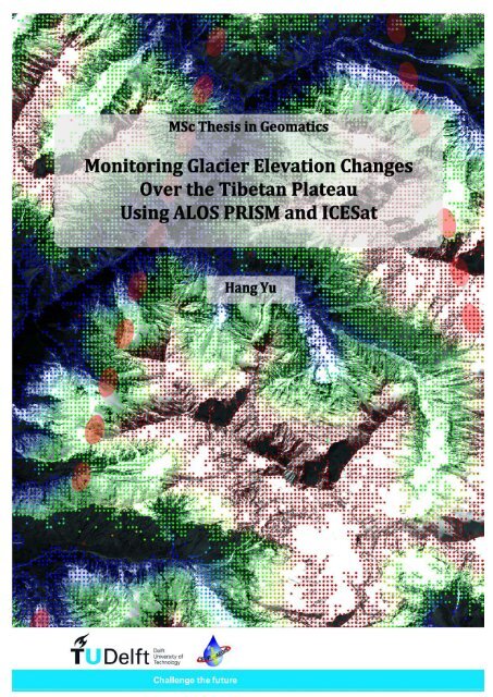
Cover image: The background is ALOS PRISM image. The overlapped color dots are
raw DEM (Digital Elevation Model) point cloud generated from ALOS PRISM. The
color presents elevations from lower to higher colored from blue to red. The tracks
of ellipses are the ICESat footprints.

Monitoring Glacier Elevation Changes
Over the Tibetan Plateau
Using ALOS PRISM and ICESat
Hang Yu
9 November, 2010
MSc Geomatics
Optical & Acoustic Remote Sensing Section
Department of Remote Sensing
Faculty of Aerospace Engineering
Delft University of Technology
The Netherlands
Graduation Committee:
Prof. dr. ir. P. J. M. van Oosterom
Prof. dr. M. Menenti
Dr. R. C. Lindenbergh
Dr. K. Khosh Elham
Dr. A. J. Hooper
Chairman
Graduation Professor
Supervisor
Supervisor
Co-reader

Contents
LIST OF TABLES ·····················································································································V
LIST OF FIGURES ················································································································· VII
CHAPTER 1 INTRODUCTION ··································································································· 1
1.1 BACKGROUND ............................................................................................................................................................... 1
1.2 PROBLEM STATEMENT AND RESEARCH QUESTION ................................................................................................. 2
1.3 RESEARCH OUTLINE ..................................................................................................................................................... 2
CHAPTER 2 THE TIBETAN PLATEAU ······················································································· 3
2.1 GENERAL INFORMATION ............................................................................................................................................. 3
2.2 THE EFFECTS OF GLOBAL WARMING ......................................................................................................................... 4
2.3 CLIMATE ........................................................................................................................................................................ 6
2.4 GLACIERS ....................................................................................................................................................................... 8
2.4.1 GLACIERS OVER TIBETAN PLATEAU ....................................................................................................... 8
2.4.2 GLACIER TERMINOLOGY (MOLNIA, 2004) ........................................................................................... 9
2.4.3 SOME FACTS ............................................................................................................................................. 10
CHAPTER 3 GLACIER OBSERVATION METHODS AND RESULTS ·············································· 15
3.1 GLACIER OBSERVATION METHODS ON THE TIBETAN PLATEAU ....................................................................... 15
3.2 MASS BALANCE EVALUATION METHODS................................................................................................................ 17
3.2.1 MASS BALANCE ........................................................................................................................................ 17
3.2.2 CALCULATIONS ........................................................................................................................................ 18
3.3 RESEARCH AREAS AND RESULTS ............................................................................................................................. 20
CHAPTER 4 DEM CONCEPTS, PRINCIPLES AND TOOLS ·························································· 23
4.1 DEM, DSM, AND DTM ............................................................................................................................................ 23
4.2 DIGITAL TERRAIN DATA ACQUISITION METHODS ................................................................................................. 24
4.2.1 DIGITIZATION OF EXISTING TOPOGRAPHIC MAPS .............................................................................. 24
4.2.2 FIELD SURVEYING (TACHEOMETRY, GPS) .......................................................................................... 25
4.2.3 PHOTOGRAMMETRY................................................................................................................................ 25
4.2.4 LASER RANGING (LIDAR)..................................................................................................................... 26
4.2.5 RADARGRAMMETRY AND SAR (SYNTHETIC APERTURE RADAR) INTERFEROMETRY................. 27
4.2.6 COMPARISON ........................................................................................................................................... 28
4.3 PHOTOGRAMMETRIC PRINCIPLES FOR DEM GENERATION ................................................................................ 29
4.3.1 IMAGING GEOMETRY OF SATELLITE PUSHBROOM IMAGE ................................................................. 29
4.3.2 IMAGE POINT MEASUREMENT ............................................................................................................... 32
4.3.3 SENSOR MODEL........................................................................................................................................ 33
4.3.4 FORWARD INTERSECTION ...................................................................................................................... 36
4.3.5 DEM MATCHING ..................................................................................................................................... 36
4.4 GROUND CONTROL POINTS (GCPS) ...................................................................................................................... 37
4.5 DEM QUALITY FACTORS AND DEM VALIDATION ................................................................................................ 38
i

ii
CONTENTS
CHAPTER 5 DATA AVAILABILITY RESEARCH ········································································ 39
5.1 AVAILABLE DEMS OVER TIBETAN PLATEAU ....................................................................................................... 39
5.1.1 ASTER GDEM ........................................................................................................................................ 40
5.1.2 SRTM........................................................................................................................................................ 40
5.1.3 GTOPO30 ............................................................................................................................................... 41
5.1.4 ACCURACY DISCUSSION ........................................................................................................................... 42
5.2 HIGH RESOLUTION SATELLITE STEREO IMAGES .................................................................................................... 43
5.3 AVAILABLE ELEVATION DATASETS ......................................................................................................................... 44
CHAPTER 6 ALOS PRISM AND ICESAT ··················································································· 47
6.1 ICESAT ........................................................................................................................................................................ 47
6.2 ALOS PRISM ............................................................................................................................................................ 49
6.2.1 ALOS AND PRISM ................................................................................................................................. 49
6.2.2 SENSOR STRUCTURE................................................................................................................................ 51
6.2.3 DATA FORMATS AND PRODUCTS ........................................................................................................... 53
6.2.4 IMAGE NOISE ............................................................................................................................................ 61
6.3 SOFTWARES CAPABLE TO HANDLE ALOS PRISM ............................................................................................... 62
6.4 DATA OVERVIEW........................................................................................................................................................ 64
CHAPTER 7 METHODOLOGY AND WORKFLOW ····································································· 67
7.1 DATASETS ................................................................................................................................................................... 67
7.2 SOFTWARE .................................................................................................................................................................. 67
7.3 PRODUCTS AND SENSOR MODEL .............................................................................................................................. 68
7.3.1 CHOOSE PROPER LEVEL OF ALOS PRISM .......................................................................................... 68
7.3.2 PROPER MODEL FOR DEM GENERATION ............................................................................................ 69
7.4 REFERENCE SYSTEM .................................................................................................................................................. 70
7.5 GROUND CONTROL POINTS (GCPS) ........................................................................................................................ 70
7.5.1 ICESAT GCPS .......................................................................................................................................... 71
7.5.2 TOPOGRAPHIC GCPS............................................................................................................................... 74
7.6 GENERATE DEM........................................................................................................................................................ 75
7.7 DEM VALIDATION METHODS ................................................................................................................................... 76
CHAPTER 8 RESULTS AND VALIDATIONS·············································································· 77
8.1 TDEM OVERALL EVALUATION USING ASTER GDEM........................................................................................ 77
8.1.1 TDEM–1B2R OVERALL ACCURACY .................................................................................................... 77
8.1.2 TDEM–1B1 OVERALL ACCURACY ....................................................................................................... 79
8.2 VALIDATIONS USING ICESAT DATA ........................................................................................................................ 84
CHAPTER 9 CONCLUSIONS, DISCUSSIONS AND RECOMMENDATIONS ···································· 91
9.1 CONCLUSIONS ............................................................................................................................................................. 91
9.2 DISCUSSIONS .............................................................................................................................................................. 92
9.3 RECOMMENDATIONS ................................................................................................................................................. 93
ACKNOWLEDGEMENTS ········································································································ 95
CONTACT INFORMATION ····································································································· 97
BIBLIOGRAPHY ···················································································································· 99
APPENDIX A A LIST OF TOPOGRAPHY NAMES ····································································· 103
APPENDIX B GLACIER LIST UPDATE ··················································································· 105

CONTENTS
iii
APPENDIX C MANUAL: ALOS PRISM LEVEL 1A/1B1 DEM GENERATION IN ERDAS LPS 9.3 ···· 107
APPENDIX D GROUND CONTROL POINTS PROFILES ···························································· 111

List of Tables
TABLE 2-1 PERCENTAGE OF RETREATING AND EXPANDING GLACIERS IN HIGH ASIA IN DIFFERENT
PERIODS (YAO, ET AL., 2004) ......................................................................................................................................... 5
TABLE 2-2 STATISTICS OF MOUNTAIN GLACIERS ON TIBETAN PLATEAU (LIU, ET AL., 2000) .............. 8
TABLE 2-3 COMPARISONS OF OBSERVED MONTHLY DATA BETWEEN 2007 AND 2008 (ZHADANG
GLACIER) (KANG, ET AL., 2009)................................................................................................................................. 13
TABLE 3-1 GLACIER LIST ........................................................................................................................................................ 21
TABLE 3-2 OBSERVATION RESULTS FOR GLACIERS ................................................................................................. 22
TABLE 4-1 A COMPARISON OF VARIOUS DTM ACQUISITION METHODS (LI, ET AL., 2004) ................... 29
TABLE 5-1 DATA AVAILABILITY RESEARCH (GREEN: AVAILABLE GLOBAL DEMS; YELLOW:
AVAILABLE HIGH RESOLUTION SATELLITE STEREO IMAGES; BLUE: OTHER AVAILABLE
ELEVATION DATASETS) ................................................................................................................................................ 45
TABLE 6-1 GLAS DATA CAMPAIGNS FROM 2003 TO 2008 (DUONG, 2010) .................................................... 48
TABLE 6-2 PRISM OBSERVATION MODES....................................................................................................................... 50
TABLE 6-3 CEOS FORMAT FILES AND FILE NAMES (EORC, JAXA, 2007) ......................................................... 53
TABLE 6-4 LEVEL DEFINITION OF PRISM STANDARD DATA PRODUCTS AND DELIVERED FORMAT
(JAXA, 2008) ........................................................................................................................................................................ 54
TABLE 6-5 COORDINATE TRANSFORMATION FUNCTION (JAXA, 2008) .......................................................... 58
TABLE 6-6 DEM GENERATION SOFTWARE .................................................................................................................... 63
TABLE 6-7 ICESAT FILE LIST ................................................................................................................................................. 65
TABLE 7-1 DATA REFERENCE SYSTEM OVERVIEW ................................................................................................... 70
TABLE 8-1 TDEM-1B2R GCPS TRIANGULATION RESULT ........................................................................................ 78
TABLE 8-2 TDEM-1B2R CHECK POINTS TRIANGULATION RESULT................................................................... 78
TABLE 8-3 TDEM-1B2R MINUS GDEM STATISTICS .................................................................................................... 79
TABLE 8-4 LEVEL 1B1 GCPS TRIANGULATION RESULT .......................................................................................... 80
TABLE 8-5 LEVEL 1B1 CHECK POINTS TRIANGULATION RESULT ..................................................................... 80
TABLE 8-6 TDEM MINUS GDEM DIFFERENCE STATISTICS .................................................................................... 81
TABLE 8-7 LOCAL ANALYSIS OF TDEM MINUS GDEM .............................................................................................. 82
TABLE 8-8 VALIDATION WITH CAMPAIGN L3K. (ELLIPSE: ICESAT L3K POINTS FOOTPRINT; POINTS:
TDEM-1B1-6; BACKGROUND RASTER PIXELS: ASTER GDEM (30 M CELL SIZE)) ............................. 86
TABLE A-1 PROPER NAME COMPARISON ..................................................................................................................... 103
v

List of Figures
FIGURE 2-1 TIBETAN PLATEAU (WIKIPEDIA) ................................................................................................................. 4
FIGURE 2-2 BASIN BOUNDARIES AND RIVER COURSES OF THE INDUS, GANGES, BRAHMAPUTRA,
YANGTZE, AND YELLOW RIVERS. BLUE AREAS DENOTE AREAS WITH ELEVATION EXCEEDING
2000 MASL (METER ABOVE SEA LEVEL). THE DIGITAL ELEVATION MODEL IN THE
BACKGROUND SHOWS THE TOPOGRAPHY RANGING FROM LOW ELEVATIONS (DARK GREEN)
TO HIGH ELEVATIONS (BROWN). (IMMERZEEL, ET AL., 2010) .................................................................... 5
FIGURE 2-3 SEASONAL SNOW COVER (WINTER (TOP), SPRING, SUMMER, AUTUMN (BOTTOM))
BASED ON MOD10C2 SNOW COVER TIME SERIES FROM MARCH 2000 TO FEBRUARY 2008. THE
VALUES SHOW THE PERCENTAGE OF TIME THAT A PIXEL WAS SNOW COVERED DURING THE
SPECIFIED SEASON WITHIN THE ENTIRE TIME SERIES, (IMMERZEEL, ET AL., 2009). ..................... 7
FIGURE 2-4 DISTRIBUTION OF GLACIERS IN THE TIBETAN PLATEAU (WWF NEPAL PROGRAM, 2005)
...................................................................................................................................................................................................... 9
FIGURE 2-5 GLACIER CHANGE CHARACTERS IN HIGH ASIA (M/YEAR) (YAO, ET AL., 2004) ................ 11
FIGURE 2-6 SENSITIVITY TYPES OF GLACIERS AND THEIR DISTRIBUTION IN CHINA (DUAN, ET AL.,
2009) ...................................................................................................................................................................................... 12
FIGURE 3-1 AN EXAMPLE OF A FIELD MEASUREMENT WITH MARKER POLES ON 4800 M BY THE
CAREERI RESEARCHERS ON YULONG SNOW MOUNTAIN (XINHUANET) ............................................. 16
FIGURE 3-2 GREENLAND ICE SHEET PROJECT 2 (GISP2) ICE CORE FROM 1837 M DEPTH WITH
CLEARLY VISIBLE ANNUAL LAYERS (WIKIPEDIA) ........................................................................................... 17
FIGURE 3-3 JULY 1979 PHOTOGRAPH OF A 9 METER DEEP SNOW PIT DUG INTO THE 1978-1979
THICK SNOW ACCUMULATION THAT FELL ON THE SURFACE OF THE TAKU GLACIER, JUNEAU
ICEFIELD, TONGASS NATIONAL FOREST, COAST MOUNTAINS, ALASKA. THE THICKNESS AND
DENSITY OF THE NEW SNOW IS BEING MEASURED TO DETERMINE ITS VOLUME AND WATER
CONTENT, AS WELL AS TO STUDY ITS METAMORPHISM TO GLACIER ICE. (MOLNIA, 2004) ..... 18
FIGURE 3-4 NYAINQENTANGLHA MT. AND NAM CO LAKE. (GOOGLE SATELLITE IMAGE) .................... 20
FIGURE 4-1 A CLASSIFICATION SCHEME OF REPRESENTATION OF DIGITAL TERRAIN SURFACES (LI,
ET AL., 2004) ....................................................................................................................................................................... 24
FIGURE 4-2 PHOTOGRAMMETRIC PROCESS (KHOSHELHAM, 2009) ................................................................. 26
FIGURE 4-3 FULL WAVEFORM LASER ALTIMETRY (DUONG, ET AL., 2009) .................................................. 27
FIGURE 4-4 PUSHBROOM SCANNER (ALONG TRACK SCANNER) (SABINS JR., 1986) ................................ 30
FIGURE 4-5 INTERIOR ORIENTATION OF SATELLITE PUSHBROOM IMAGE (LEICA, 2005) ................... 31
FIGURE 4-6 IMAGE COORDINATES IN A SATELLITE SCENE (LEICA, 2005) .................................................... 31
FIGURE 4-7 VELOCITY VECTOR AND ORIENTATION ANGLE OF A SINGLE SCENE (LEICA, 2005) ....... 32
FIGURE 4-8 MANUALLY IMAGE POINT MEASUREMENT IN ERDAS LPS 9.3 USING ALOS PRISM
OVERLAPPING IMAGES (APPENDIX D) .................................................................................................................. 33
FIGURE 4-9 SENSOR MODEL PARAMETERS (LEICA, 2005) .................................................................................... 34
FIGURE 4-10 IMAGE PYRAMID FOR MATCHING AT COARSE TO FULL RESOLUTION (LEICA, 2005) . 37
FIGURE 5-1 SHADED RELIEF IMAGES COMPUTED FOR A MOUNTAINOUS AREA IN CENTRAL
COLORADO. IMAGES COMPARE THE ASTER GDEM (1 ARC-SECOND /30 METER) IN THE
CENTER WITH TWO VERSIONS OF THE SRTM DEM (3 ARC-SECOND / 90 METER) (LEFT) AND
THE 1 ARC-SECOND / 30 METER (RIGHT). (MICROIMAGES,INC, 2009)................................................. 42
vii

viii
LIST OF FIGURES
FIGURE 6-1 PRINCIPAL OF OPERATING OF ICESAT (DUONG, ET AL., 2009) ................................................... 48
FIGURE 6-2 OVERVIEW OF ALOS (JAXA, 2008) ............................................................................................................. 49
FIGURE 6-3 OVERVIEW OF PRISM (EORC, JAXA, 2007) ............................................................................................. 50
FIGURE 6-4 PRISM OBSERVATION MODES (OB1 AND OB2) (EORC, JAXA, 2007) ......................................... 50
FIGURE 6-5 OB1 STEREO IMAGE GEOMETRY (KÄÄB, 2008) .................................................................................. 51
FIGURE 6-6 OB2 STEREO PAIR GEOMETRY (RECREATED BASED ON (KÄÄB, 2008)) ................................ 51
FIGURE 6-7 PRISM OBSERVATION CONCEPT (RECREATED BASED ON (JAXA, 2008)) .............................. 52
FIGURE 6-8 LINEAR ARRAY CCD STRUCTURE OF THE PRISM NADIR VIEWING CAMERA (KOCAMAN,
ET AL., 2007) ........................................................................................................................................................................ 53
FIGURE 6-9 LEVEL 1A DATA (NADIR 70 KM (LEFT) + BACKWARD 35 KM (RIGHT)) ................................. 55
FIGURE 6-10 DN VALUE STATISTICS OF LEVEL 1A NADIR IMAGE (LEFT) AND LEVEL 1B1 NADIR
IMAGE (RIGHT) USING BEAM 4.7.1 ........................................................................................................................... 55
FIGURE 6-11 CCD BOUNDARY SEEN IN LEVEL 1A DATA (LEFT) WHICH IS CORRECTED IN LEVEL 1B1
(RIGHT) .................................................................................................................................................................................. 55
FIGURE 6-12 LEVEL 1B1 IMAGE STRUCTURE (ABOVE: NADIR IMAGE; BELOW: BACKWARD IMAGE)
.................................................................................................................................................................................................... 57
FIGURE 6-13 CONCEPT OF THE PRISM GEO-CORRECTION (JAXA, 2008) ......................................................... 59
FIGURE 6-14 LEVEL 1B2R IMAGE STRUCTURE (ABOVE: NADIR IMAGE; BELOW: BACKWARD IMAGE)
.................................................................................................................................................................................................... 60
FIGURE 6-15 LEVEL 1B2G IMAGE (LEFT: NADIR IMAGE; RIGHT: BACKWARD IMAGE) ............................ 61
FIGURE 6-16 STRIP NOISE REDUCE BEFORE (LEFT) AND AFTER (RIGHT) (KAMIYA, 2008) ................. 61
FIGURE 6-17 JPEG NOISE FOUND IN LEVEL 1A, 1B1, 1B2R (LEFT TO RIGHT) ............................................... 62
FIGURE 6-18 ALOS PRISM DATA COVERAGE AVAILABLE VIA ESA ...................................................................... 64
FIGURE 6-19 RESEARCH AREA OF THIS THESIS ........................................................................................................... 64
FIGURE 6-20 PRISM AND ICESAT DATA OVERVIEW................................................................................................... 65
FIGURE 7-1 ORTHOGRAPHIC VIEWS PROJECT AT A RIGHT ANGLE TO THE DATUM PLANE.
PERSPECTIVE VIEWS PROJECT FROM THE SURFACE ONTO THE DATUM PLANE FROM A FIXED
LOCATION. (WIKIPEDIA) ............................................................................................................................................... 69
FIGURE 7-2 LPS 9.3 MODEL SETUP ..................................................................................................................................... 69
FIGURE 7-3 ICESAT L3I TRACKS IN ALOS PRISM OVERLAP REGION .................................................................. 71
FIGURE 7-4 ELEVATION PROFILE COMPARISON BETWEEN ICESAT AND ASTER GDEM OF L3I LEFT
TRACK AND RIGHT TRACK ........................................................................................................................................... 72
FIGURE 7-5 FILTERED ICESAT L3I LEFT AND RIGHT TRACKS .............................................................................. 73
FIGURE 7-6 ICESAT L3K LEFT TRACK BEFORE AND AFTER FILTERING .......................................................... 74
FIGURE 7-7 GCPS ON CONTOUR MAP................................................................................................................................. 75
FIGURE 7-8 DEM GENERATION WORK FLOW IN LP ................................................................................................... 76
FIGURE 8-1 TDEM-1B2R-41 (LEFT) AND ITS DIFFERENCE MAP WITH ASTER GDEM (RIGHT) ............ 79
FIGURE 8-2 TDEM-1B1 POINT CLOUD AND THE SAME AREA ASTER GDEM RASTER MAP ..................... 81
FIGURE 8-3 TDEM-1B1-6 MINUS ASTER GDEM WITH 4 LOCAL STATISTICS AREA ..................................... 82
FIGURE 8-4 TDEM POINT CLOUD OVERLAYING ALOS PRISM NADIR IMAGE SHOWS THE
MISMATCHED AREA ......................................................................................................................................................... 84
FIGURE 8-5 L3K PROFILES AND VALIDATION POINTS ............................................................................................. 85
FIGURE 8-6 224 ICESAT POINTS SAMPLE: ....................................................................................................................... 88
FIGURE 8-7 138 ICESAT POINTS SAMPLE: ....................................................................................................................... 89
FIGURE 8-8 60 ICESAT POINTS SAMPLE: ......................................................................................................................... 89
FIGURE 8-9 24 ICESAT POINTS SAMPLE. .......................................................................................................................... 90
FIGURE C-1 MODEL SETUP ................................................................................................................................................... 107
FIGURE C-2 BLOCK PROPERTY SETUP ........................................................................................................................... 108
FIGURE C-3 ADD FRAMES ..................................................................................................................................................... 108
FIGURE C-4 IMPORT POINTS ............................................................................................................................................... 109

Abstract
Glacier melting has become a key issue in the current discussion on global climate change.
Glaciers of the Tibetan Plateau may be heavily affected by global warming. Hence, possible
glacier melting over the plateau attracts the most attention. Possible glacier melting is evaluated
via studies on mass balance of the glaciers. Glacier elevation change is an important parameter
in mass balance assessments. Traditional observations of glacier elevation changes were
acquired by surveying. As an example, a large elevation change of 1.5 m decrease was reported
at Zhadang glacier on the southwest Tibetan Plateau between 2005 and 2006. Traditional
surveying is expensive for large areas and is limited by the extreme terrain and weather
conditions on the Tibetan plateau. Therefore, remote sensing techniques are preferred in the
research on ongoing glacier elevation changes.
The research method assessed here considers elevation changes obtained by comparing serial
DEMs. Photogrammetry techniques are applied for DEM generation. The 2.5 m horizontal
resolution satellite images of the ALOS PRISM instrument are used as base image. One PRISM
scene centered at longitude 81°15´37”N and latitude 29°49´53”E, available at both Level 1A/1B
and Level 1B2R/1B2G, is employed for DEM and quality evaluation. ICESat laser altimetry data
from campaign L3I is selected as ground control points (GCPs). ICESat has decimeter vertical
accuracy over flat terrain In this case ICESat elevations are chosen as GCPs because sufficient
GCPs from other sources are not available. The DEM generation is performed in the ERDAS LPS
9.3 software. The quality of the resulting TDEM (Tibetan Plateau DEM) is evaluated by ASTER
GDEM and by data from different ICESat campaigns. Compared with ASTER GDEM, the mean
difference is -41 meters. The TDEM has a mean difference of 5-10 meters with ICESat data from
campaigns L3H, L3J and L3K. It is concluded that TDEM’s accuracy is sufficient to detect 15 m
elevation change in 10 year’s time, which correspond to an annual glacier elevation change rate
of 1.5 meters. The accuracy of TDEM is notably better than ASTER GDEM. As one TDEM tile
reports the elevation of a glacier at a clear moment in time, TDEM is more suitable than ASTER
GDEM for glacier mass balance studies.
ix

Chapter 1
Introduction
Glacier melting has become a key issue in the current discussion on global climate change.
Glaciers of the Tibetan Plateau may be heavily affected by global warming. Hence, possible
glacier melting over the plateau attracts the most attention. Possible glacier melting is evaluated
via studies on mass balance of the glaciers. Glacier elevation change is an important parameter
in mass balance assessments. Traditional observations of glacier elevation changes were
acquired by surveying, which is expensive for large areas and is limited by the extreme terrain
and weather conditions on the Tibetan plateau. Remote sensing techniques are applied mostly in
the research of glacier area changes. Therefore, a sufficient method needs to be researched to
detect glacier elevation changes.
1.1 Background
The research is part of the CEOP-AEGIS project partly carrying on in TU Delft. CEOP-AEGIS
stands for “Coordinated Asia-European long-term Observing system of Tibetan Plateau
hydro-meteorological processes and the Asian-monsoon systEm with Ground satellite Image
data and numerical Simulations”. The project started from 01/05/2008 and will go on till
01/05/2012.
Some studies are done by the TU Delft group. Hieu Duong finished the inventory of available
ICESAT laser altimetry data over Tibetan Plateau. BSc student Simon Billemont researched on
evaluation of the ASTER GDEM by comparing ICESAT data over the flat Nam Co Lake and the
area between 90° - 91°E and 31° - 37°N. Master student Lennert van den Berg is trying to evaluate
the horizontal and vertical glacier changes by looking into the time series of ICESAT data and
SAR based horizontal flow velocities. Other studies are in progress at the same time. Dr. Roderik
Lindenbergh is studying on the methods to compare sparse ICESAT footprints in time series.
(CEOP-AEGIS, 2009)
Glacier melting is one issue under the fact of global warming. The glaciers give the direct
response to the growing temperature. The diminishing glaciers frighten humans with all kinds of
worries, because the glaciers are the key containers for fresh water. It records the climate
changes and at the same time influences the climate. Research on glaciers is helpful to evaluate
and forecast the effects of the global warming.
Within all the glaciers, the huge amount in Tibetan Plateau attracts the attention of people all
over the world. Previous studies showed significant warming in the Tibetan Plateau during the
1

2 1.2 PROBLEM STATEMENT AND RESEARCH QUESTION
last half century, which is projected to continue in the future at a faster rate than the global mean
(Kang, et al., 2010). The rapidly melting of the glaciers becomes a serious problem both
regionally and globally.
1.2 Problem statement and research question
While, the Tibetan Plateau has especially rough terrain and extreme weather conditions,
traditional surveying method for elevation measurement is limited here. The challenge is to have
accurate elevation measurement for such terrain surface with remote sensing techniques. The
idea is to detect elevation changes by comparison of digital elevation models (DEMs) from two
time spots over the glacier. While, how many changes there are and whether the method is
sufficient to detect such amount of changes are the questions to be researched.
1.3 Research outline
The research has 9 chapters in total. It starts from studying the background information of the
Tibetan Plateau and the glaciers over it. In Chapter 2 and 3, the general information of the
Tibetan Plateau such as location, climate are introduced. Further, what is the role of Tibetan
Plateau in climate change, and how exactly it affects the glaciers will be answered in these two
chapters.
In order to find the suitable method, different technologies that can acquire terrain data are
studied in Chapter 4. How photogrammetric methods work and how to cope with satellite data
with photogrammetry are illustrated in details in this chapter.
Chapter 5 and 6 are data related research and studies. There gives an overview of the data
resources could be used over the Tibetan Plateau. Besides, software capable to handle these
dataset is also presented. Two dataset, ALOS PRISM and ICESat are introduced and studied in
this chapter.
Chapter 7 describes the processing flow to obtain DEM. The results are presented and evaluated
in Chapter 8. The conclusion and recommendations about the thesis are in Chapter 9.

Chapter 2
The Tibetan Plateau
In this chapter, it is getting to know the Tibetan Plateau with the general information (Section
2.1) and its unique climate (Section 2.3). The Tibetan Plateau plays an important role in the
global warming that the effects are discussed in Section 2.2. Glaciers on the Tibetan Plateau
response directly to such climate change. Knowledge about glaciers and the glacier situation
over the Tibetan Plateau are studied in Section 2.4.
2.1 General information
The Tibetan Plateau is also known as Qinghai-Tibetan (Qingzang) Plateau (Chinese: ,
Pinyin: Qingzang Gaoyuan). The whole Tibet Autonomous Region (TAR) and the Qinghai
Province of China are on it, which explains the name Qinghai-Tibetan Plateau. It also covers the
west of Sichuan Province, the south of the Xinjiang Uygur Autonomous Region and parts of
Gansu and Yunnan Province of China. The whole Tibetan Plateau covers parts of Bhutan, Nepal,
India, Pakistan, Afghanistan, Tadzhikistan, and Kyrgyzstan as well. (Wikipedia) (Baidu)
The Tibetan Plateau (Figure 2-1) lies between the Himalaya Mountains to the south and the
Taklimakan Desert to the north, and is located between 78°25' - 99°06' E and 26°44' - 36°32' N
(China Internet Information Center). It occupies an area of around 2.5 million square kilometers,
with 2.4 million square kilometers within China. It has an average elevation of 4,500 meters.
People call it “the roof of the world”, as it is the biggest plateau in China with the highest average
elevation in the world. With respect to the North Pole and South Pole, the Tibetan Plateau is also
called “the third pole” as the highest pole. (Wikipedia) (Baidu)
The plateau is bordered by mountains, on the Northwest there are the Kunlun Mountains and
the Qilian Mountains are in northeast of the plateau. Kalakunlun Mountains are in the east.
Hengduan Mountains is in the west. In the south, there are the Himalaya Mountains. Within the
plateau, there are also the Tanggula Mountains, the Gangdisi Mountains and the
Nyainqentanglha Mountain. The elevations of most mountains are over 6,000 meters. (Baidu)
It is called the “Asia water tower”, as the Tibetan Plateau is the world third-largest storage of ice.
It is the origin of many rivers which are the lifelines of the populations in Asia, like Yangtze and
Yellow river, the mother rivers of China. The Yangtze River originates from the Geladandong
Snow Mountain(33°30' N,91°30' E) which is the highest peak of Tanggula Mountain. Its basin
covers one fifth of China. The Yellow river originates from the Bayar Har Mountains. The
3

4 2.2 THE EFFECTS OF GLOBAL WARMING
Salween, Mekong, Ganges, Indus and the Brahmaputra River Rivers also originate here. (Baidu)
Figure 2-1 Tibetan Plateau (Wikipedia)
2.2 The effects of global warming
Qin Dahe, the former head of the China Meteorological Administration said: “Temperatures are
rising four times faster than elsewhere in China, and the Tibetan glaciers are retreating at a
higher speed than in any other part of the world.” “In the short term, this will cause lakes to
expand and bring floods and mudflows.” “In the long run, the glaciers are vital lifelines for Asian
rivers, including the Indus and the Ganges. Once they vanish, water supplies in those regions will
be in peril.” (Wikipedia)
A recent research shows that the meltwater is extremely important in the Indus basin and
important for Brahmaputra basin, but plays only a modest role for the Ganges, Yangtze and
Yellow rivers (Figure 2-2). The Brahmaputra and Indus basins are most susceptible to
reductions of flow, thereby threatening the food security of an estimated 60 million people.
(Immerzeel, et al., 2010)

CHAPTER 2 THE TIBETAN PLATEAU 5
Figure 2-2 Basin boundaries and river courses of the Indus, Ganges, Brahmaputra, Yangtze,
and Yellow rivers. Blue areas denote areas with elevation exceeding 2000 masl (meter above
sea level). The digital elevation model in the background shows the topography ranging from
low elevations (dark green) to high elevations (brown). (Immerzeel, et al., 2010)
Studies show that since the 1990s, the glaciers began to retreat globally (Table 2-1). The large
scale retreat started from the 1950s. In the following decades some glaciers even got a positive
mass balance. From the 1980s, retreat became faster. Then the most serious period comes,
which we are experiencing now. The most obvious case happened in the southwest Tibetan
Plateau. (Yao, et al., 2004)
Many studies show that the temperature is rising globally. And the weather records show that an
increase of precipitation in most regions of the Tibetan Plateau is happening. (China Digital
Science and Technology Museum) The glacier retreat implies loss in mass balance. Melting is the
main way for glaciers to lose mass. Temperature change is one reason to affect the melting of
glaciers. Irregular increase of the percentage of rainfall in yearly precipitation will also speed up
the melting of glaciers.
Table 2-1 Percentage of retreating and expanding glaciers in High Asia in different periods
(Yao, et al., 2004)
Period
Observed
glacier
numbers
Retreating
glacier (%)
Expanding
glaciers (%)
Stable
glaciers (%)
1950 - 1970 116 53.46 30.17 16.37
1970 - 1980 224 44.2 26.3 29.5
1980 - 1990 612 90 10 0
1990 - 2004 612 95 5 0

6 2.3 CLIMATE
2.3 Climate
In general, the climate on the Tibetan Plateau is characterized by strong solar radiation and low
temperature. The air temperature decreases with the rising of altitude and latitude. It is
estimated that for every 100 meters increase in altitude, the average annual temperature lowers
by 0.57°C. For every one degree increase in latitude, the average annual temperature lowers by
0.63°C. The temperature has a big daily range. The wet and dry seasons are clear. But the four
seasons are not clearly divided. In most parts, the warmest month average temperature is below
15°C. Normally, the average temperature in January and in July is 15-20°C lower than that at the
same latitude in the eastern plains. (China Digital Science and Technology Museum)
As the elevation of the Tibetan Plateau has a great disparity, the duration of low temperature
periods varies for different regions. In the winter half year, the weather condition is cold, dry
and windy. The lowest temperatures are mostly below -20°C. In the north and west region, the
average temperature is below zero from October to next April. In Brahmaputra River basin in
the south with an altitude below 4000 meters, the cold period lasts 2-3 months. In the southeast
region, it is below 100 days. Except for south Himalaya and the southeast region, the
precipitation is less than 80mm between November and April, less than 12% of the annual
precipitation.
In the summer half year, the average temperature is mostly below 18°C. The weather is mostly
cool and rainy. It is 10°C to 18°C in the southwest region which is below 4500 meters and the
Brahmaputra River basin. It is below 10°C on the Qiangtang Plateau with an altitude over 4500
meters. Rainfall is highly concentrated in this period, and usually accounts for 80-90% of the
whole year. Precipitation gradually reduces from southeast to northwest. In the south of the
Himalayas windward side, annual precipitation is up to 1000 mm or more. But in the narrow
strip between Himalayan northern foot and the Brahmaputra, the annual precipitation is less
than 300 mm. That is why this strip is called the "rain shadow zone.”
This typical seasonal shift of the Tibetan Plateau is caused by the well known Asia Monsoon. It is
believed that the high altitude plateau strengthens the Asia Monsoon. Monsoon is used to
describe seasonal reversals of wind direction, caused by temperature differences between the
land and sea. (BBC Weather) The Tibetan Plateau is situated at a large land mass surrounded by
large seas, the Arabian Sea and the Indian Ocean. The landmasses warm up – and cool down –
faster than large bodies of water. This means that the Tibetan Plateau warms faster than the
Indian Ocean to the south. In the summer, the warm air rises, creating an area of low pressure.
This creates a steady wind from south to north blowing towards the land, bringing moist air
from the oceans. In the winter, the landmass cools quickly, while the ocean is warmer, causing
the winds to reverse, blowing from north to south. (Wikipedia)
Figure 2-3 shows the seasonal change in snow cover on the whole Tibetan Plateau. The one on
the top is from December to February. In the same manner, the third one is from June to August.
The changes between the four figures are regionally. The global change of snow cover is obvious
between the first and the third figure. The melting of snow is from March, gradually starts from
south to north. For example, around the south-eastern lowlands, rainfall generally increases at
the beginning of March which starts the rainy season. In the north and eastern Tibetan plateau, it
starts in mid-late May. And in the Brahmaputra river basin the rainy season starts at early June.
In late June to early July the rainy season in the western Xigaz region starts.

CHAPTER 2 THE TIBETAN PLATEAU 7
Figure 2-3 Seasonal snow cover (winter (top), spring, summer, autumn (bottom)) based on
MOD10C2 snow cover time series from March 2000 to February 2008. The values show the
percentage of time that a pixel was snow covered during the specified season within the entire
time series, (Immerzeel, et al., 2009).

8 2.4 GLACIERS
2.4 Glaciers
2.4.1 Glaciers over Tibetan Plateau
Characteristics of the glaciers on the Tibetan Plateau are calculated based on the Chinese Glacier
Inventory (WDC). Statistics (Table 2-2) shows that that there are 36,793 glaciers existing on the
Tibetan Plateau, with a total area of 49,873.44 km 2 and a total ice volume of 4,561.3857 km 3 . The
Tibetan Plateau is the largest existing glaciation area in the low to mid latitude area of the world
(Liu, et al., 2000). Glaciers are distributed mainly in Kunlun Mts., Himalayas Mts. and
Nyainqentanglha Mt., reserving over half of the total glaciers on the Tibetan Plateau. Figure 2-4
shows the distribution of mountains and glaciers. Since there is a time gap for the data between
Table 2-2 and Figure 2-4, the appearance may differ from the description.
Mt. name
Table 2-2 Statistics of mountain glaciers on Tibetan Plateau (Liu, et al., 2000)
Glacier
numbers
Glacier area
Glacier reserves
Equivalent water
volume
Glacier melt
water
(%) (km 2 ) (%) (km 3 ) (%) (×10 8 m 3 ) (%) (×10 8 m 3 ) (%)
Qilian Mt. 2,815 7.7 1,930.49 3.9 93.4962 2.1 804.068 2.1 11.32 2.7
Kunlun Mt. 7,694 20.9 12,266.29 24.61 1282.9279 28.2 11,033.180 28.2 61.87 12.3
Aurjin Mt. 235 0.6 275.00 0.6 15.8402 0.3 136.225 0.3 1.39 0.3
Tanggula Mt. 1,530 4.2 2,213.40 4.4 183.8761 4.0 1,581.334 4.0 17.59 3.5
Qiangtang
Plateau
958 2.6 1,802.12 3.6 162.1640 3.6 1,394.610 3.6 9.29 1.8
Karakoram Mt. 3,454 9.4 6,230.80 12.5 686.2967 15.0 5,902.152 15.0 38.47 7.6
Hengduan Mt. 1,725 4.7 1,579.49 3.2 97.1203 2.1 835.235 2.1 49.94 9.9
Pamir Plateau 1,289 3.5 2,696.11 5.4 248.4596 5.4 2,136.753 5.4 15.35 3.0
Gangdise Mt. 3,538 9.6 1,766.35 3.5 81.0793 1.8 697.282 1.8 9.41 1.8
Nyainqentanglha
Mt.
7,080 19.2 10,701.43 21.4 1,001.5806 22.0 8,613.593 22.0 213.27 42.3
Himalaya Mts. 6,475 17.6 8,411.96 16.9 708.5448 15.5 6,093.485 15.5 76.59 15.2
Total 36,793 100 49,873.44 100 4,561.3857 100 39,227.917 100 504.49 100
As is shown in Table 2-2, the ice volume is 4,561.3857 km 3 , which is approximately equal to
39,227.917×10 8 m 3 fresh water (1 g/cm 3 ) assuming 0.86 g/cm 3 as the average ice density. This is
a huge amount of fresh water. According to the calculation, the glaciers on the Tibetan Plateau
provide an amount of melt water of 504.49×10 8 m 3 per year. The water is the main source for the
rivers that originate here.
The distribution of the water resource is uneven compared to the different locations of the
mountains on the Tibetan Plateau. It relates to the different topography and climate condition of
each individual glacier situated. For example, the amount of melt water of Hengduan Mt. and
Nyainqentanglha Mt. is relative high compared to the other mountains. Because they are in the
southwest maritime climate zone, there is more rain. Moreover higher temperatures result in
stronger melting.

CHAPTER 2 THE TIBETAN PLATEAU 9
Figure 2-4 Distribution of glaciers in the Tibetan Plateau (WWF Nepal Program, 2005)
2.4.2 Glacier terminology (Molnia, 2004)
In order to understand well and clearly the characteristics and situation of the glaciers described
in the literature, some terms are introduced briefly.
• Accumulation: The addition of ice and snow into a glacier system. This occurs through a
variety of processes including precipitation, firnification, and wind transport of snow into a
glacier basin from an adjacent area.
• Ablation: The loss of ice and snow from a glacier system. This occurs through a variety of
processes including melting and runoff, sublimation, evaporation, calving, and wind
transport of snow out of a glacier basin.
• Line of balance (LOB): Is often used in the glacier elevation change contour map. By this
division, the contour line values on one side are negative and positive on the other side.
• Mass balance: A measure of the change in mass of a glacier at a certain point for a specific
period of time. It is the balance between accumulation and ablation, also called Mass
Budget.
• Terminus: The lower-most margin, end, or extremity of a glacier. Also called
Toe, End or Snout.

10 2.4 GLACIERS
• Retreat: A decrease in the length of a glacier compared to a previous point in time. As ice in
a glacier is always moving forward, its terminus retreats when more ice is lost at the
terminus to melting and/or calving than reaches the terminus.
• Advance: An increase in the length of a glacier compared to a previous point in time. As ice
in a glacier is always moving forward, a glacier's terminus advances when less ice is lost due
to melting and/or calving than the amount of yearly advance.
• Thinning: The thinning of a glacier due to the melting of ice. This loss of thickness may
occur in both moving and stagnant ice.
• Snow Water Equivalent (SWE): Is the amount of water contained within the snowpack. It
can be thought of as the depth of water that would theoretically result if you melted the
entire snowpack instantaneously. [SWE] ÷ [Snow Density] = Snow Depth. (USDA)
• Ice core: An ice core is a core sample from the accumulation of snow and ice over many
years. Typical ice cores are removed from an ice sheet. The length of the record depends on
the depth of the ice core and varies from a few years up to 800 thousand years. The time
resolution (i.e. the shortest time period which can be accurately distinguished) depends on
the amount of annual snowfall (Wikipedia)
2.4.3 Some facts
From the literatures, some facts influencing the glacier mass balance, and rules concluded by the
experts are listed in points below. Some have already been mentioned above. Here we will give
more examples.
• Glaciers in the border retreat stronger than in the middle of the Tibetan Plateau. (Yao,
et al., 2004)
Figure 2-5 shows the glacier retreat values over the whole plateau. Because of different
topography and climate conditions, glaciers behave differently. In the middle of the plateau,
around Kunlun Mt. and Tanggula Mt., the horizontal retreat is smaller, within 10 meters per
year. From the middle to the border, the retreat becomes stronger. In the Karakoram region,
the retreat speed reaches to 30 m/year. The strongest retreat happens near the southeast
border of the plateau, where it reaches up to 40 meters. (The green parts are the sample
observation areas, from which the map is interpolated).
As a complement to the above study, a study illustrated in Figure 2-6 puts forward a
classification of the sensitivity of glaciers melting, with regards to the glacier type, the
retreat speed of each glacier region and the climate condition around the location of the
glaciers. The sensitivity of glaciers to the climate change are classified into
Extremely-sensitive, Semi-sensitive, Semi-steady and Extremely-steady. The result is
similar and comparable with Figure 2-5. In this result, the west part of Qilian Mts. and
western Nyainqentanglha Mts. are extremely sensitive.

CHAPTER 2 THE TIBETAN PLATEAU 11
Figure 2-5 Glacier change characters in High Asia (m/year) (Yao, et al., 2004)

12 2.4 GLACIERS
Figure 2-6 Sensitivity types of glaciers and their distribution in China (Duan, et al., 2009)
• More glaciers are on North Slope than South Slope of the mountains. (Yao, et al., 2004)
Most of the glaciers on the Tibetan Plateau follow this rule except Nyainqentanglha Mt. and
Gangdise Mt. The main reason is that the North Slope gets less solar radiant heat than the
South Slope, which benefits the glacier growth. But Nyainqentanglha Mt. is situated such
that southwest monsoon has large influence. The south slope is facing the wind which
brings more precipitation offsetting the melting. So in Nyainqentanglha Mt. region, there are
more glaciers on the South Slope. Gangdise Mt. is behaving similar situation, the number of
glaciers is higher on the South Slope, but the storage of the glaciers is less, since the
accumulation is less than that in Nyainqentanglha Mt. region.
• Small glaciers are more sensitive than large glaciers. (Liu, et al., 2000)
Large scale glaciers are glaciers with areas over 100 km 2 . The areas of small glaciers are
only 0.28 km 2 on average. Large glaciers are crucial for water storage and more important
from an environmental view point. But small glaciers show quicker response to climate
change. Researches on small glaciers will be helpful to forecast further effects of global
warming.

CHAPTER 2 THE TIBETAN PLATEAU 13
• The higher the elevation, the lower the glacier melting speed. (Zhou, et al., 2007)
The temperature decreases with increasing elevation. And because of the lower
temperature, the snow cover is relative thicker. In the study of the Zhadang glacier, it is
found that with higher altitude, the speed of glacier melting is also lower than on the lower
altitude part.
• Not only the growing temperature, but also the rainfalls speed up the glacier melting.
(Yang, et al., 2008)
The rapid increase in temperature results in a decline of the snow/rain ratio in the
precipitation. It becomes another factor that attributes to the shrinking of glaciers and a
strong negative mass balance was observed during the study of Kangri Kabu region. After
the snow cover on top of the glaciers was disappeared, the ability of light reflection declines.
The ice will absorb more solar radiation. The temperature and liquid precipitation are the
two main factors in the procedure of glacier melting.
• Early start of the rainy season suppresses glacier melt. (Kang, et al., 2009)
The study carried on by KANG and others in 2009 suggested that “the early rainy season in
2008 contributed to low summer temperature, causing reduced loss of glacier ice and a
surplus mass balance in 2008. The early rainy season suppressed summer glacier melt”.
Table 2-3 shows that the negative mass balance is smaller in 2008 than in 2007 on Zhadang
glacier. According to the study, “onset of rainy season should be considered when applying
glacier change studies to issues such as global warming, especially in monsoon regions with
summer precipitation”.
Table 2-3 Comparisons of observed monthly data between 2007 and 2008 (Zhadang glacier)
(Kang, et al., 2009)
May June July August September
Air
temperature
(°C)
Cumulative
temperature
above 0°C(°C)
Precipitation
(mm)
Mass balance
(mm)
Total runoff
(10 6 m 3 )
2007 2008 2007 2008 2007 2008 2007 2008 2007 2008
-1.34 -2.35 0.73 0.87 2.70 2.21 2.29 1.36 0.42 -0.36
21.66 3.95 41.17 36.99 83.82 68.63 71.05 43.44 22.88 10.31
13.1 33.0 44.2 110.0 145.0 145.0 145.8 110.6 69.6 76.6
449 312 -346 174 -399 -178 -375 5 -112 -90
- - 1.11 1.04 4.13 1.76 2.86 1.82 0.94 1.41

Chapter 3
Glacier Observation Methods and Results
This chapter will focus on the glaciers over the Tibetan Plateau. Studies on glacier mass balance
(Section 3.2) are researched in this chapter. In these literatures, different methods (Section 3.1)
are implemented to measure the glaciers and glacier changes. Section 3.3 presented the
observation results of the glaciers over the Tibetan Plateau.
3.1 Glacier Observation methods on the Tibetan Plateau
The observation records of glaciers on the Tibetan Plateau were available since 1950s. More
records can be found since the 1980s. The field observation conditions on the high elevation
plateau are hard. The extreme temperature and weather conditions make it harder to carry out
measurements. Measurements can hardly cover large areas, since not all the areas are reachable.
The results and records are limited to individual glaciers. With the development of earth
observation instruments and platforms, large area monitoring is getting possible with precise
remote sensing instruments.
The issue on glacier study is to get the basic glacier parameters for evaluating the glaciers, most
common are glacier area and elevation. Additional glacier parameters that can be derived from
space borne sensors include mapping of snowlines and flow velocity. An issue for glacier
observation is to measure the line of balance (LOB). (Racoviteanu, et al., 2009) Remote sensing
techniques are commonly used in mapping clean ice, glacier lakes, and debris-covered ice, DEM
generation, and change detection.
In previous research on the Tibetan Plateau glaciers, field observations are commonly used and
resulted in measuring LOB, and basic glacier parameters such as location, length and area. From
these results, the ice volume can be estimated but only for glaciers with a limited area. Also a lot
of measurements with remote sensing are carried on. The latest results over the Tibetan Plateau
are more about glacier mapping, including classification and boundary mapping, and DEM
generation using remote sensing data. Here is a list of the methods used for obtaining the
observation results got in Table 3-1 and Table 3-2.
• Field observation with marker poles
In the study of Zhadang glacier (Zhou, et al., 2007), poles are used. The poles are settled at
different topographic height levels to measure the length change of the marker, snow cover
15

16 3.1 GLACIER OBSERVATION METHODS ON THE TIBETAN PLATEAU
thickness and density, subjoin glacier thickness, and polluted layer thickness. Two
Automatic Weather Stations (AWS) are used to get simultaneous temperature collection.
The marker posts may fall over due to the moving or melting of the glaciers, therefore,
additional maker poles need to be added during the warm season. The method needs
human effort to keep enough marker poles and maintain them in good condition. The
accuracy is low because the poles may deform or be destroyed due to the strong wind or
extreme temperatures, and the moving of the glaciers. It is the most direct method to get
first hand measurements. But it is hard to obtain a long time series of measurement. Usually
this method is used for a few years long only. Figure 3-1 shows an example of how the
marker poles work in the field.
With the marker poles, the accumulation and ablation values of the snow cover and glaciers
can be measured. This method will result in a contour map of the accumulation and ablation
values and consecutively in the line of balance, and a first mass balance estimate. The mass
balance evaluation method used in (Zhou, et al., 2007) is explained in Paragraph 3.2.2.
Figure 3-1 An example of a field measurement with marker poles on 4800 m by the CAREERI
researchers on Yulong Snow Mountain (XINHUANET)
• Ice core
Ice cores (Figure 3-2) record the climate changes history. A sample ice core study is helpful
in forecasting and analyzing the weather changes. An ice core from the right location can be
used to reconstruct an uninterrupted and detailed climate record extending over hundreds
of thousands of years, providing information on a wide variety of aspects of climate at each
point in time (Wikipedia). But the sample results cannot give a quantitative evaluation. Ice
core samples from different glaciers are used to study the climate change over the Tibetan
Plateau in the recent a hundred years. (Pu, et al., 2004)

CHAPTER 3 GLACIER OBSERVATION METHODS AND RESULTS 17
Figure 3-2 Greenland Ice Sheet Project 2 (GISP2) ice core from 1837 m depth with clearly
visible annual layers (Wikipedia)
• Field observations with GPS
GPS is often used together with other observation methods. It is the most available tool to
get the location and elevation of glaciers. It is used to survey the location of the terminus for
each glacier, e.g. one time each year to monitor the retreat of glaciers. The method needs
human effort and the glaciers should be reachable. GPS is commonly used in study the
Tibetan Plateau glacier, for example in the study of (Kang, et al., 2007) and (Yang, et al.,
2008) inTable 3-2.
• Ground Penetrating Radar(GPR) glacier thickness measurement
GPR is normally used in layer structure detection and object detection. It is used on glaciers
to measure the thickness and estimate the volume. It also needs a direct access. In (Ma, et al.,
2008) ‘s study on the south Tibetan Plateau Guren Hekou glacier, GPR is used to evaluate
the mass balance. The method is explained in Paragraph 3.2.2.
• Aero photos
In 1970s, a large scale survey over the Tibetan Plateau was carried out using aero
photogrammetry. The China Glacier Inventory is made based on this measurement. A lot of
studies comparing the glacier changes (like the study of glacier retreat length (Kang, et al.,
2007) in Table 3-2) with 1970s use this dataset. It plays a significant role even today in
many studies comparing the glacier changes in time series.
• Remote sensing
Remote sensing images are often used in glacier mapping, like Landsat TM/+ETM in the
Western Qilian Mountains (Liu, et al., 2002), in the Western Nyainqentanglha Mt. (Shang
Guan, et al., 2008), and MODIS in the Himalayan river basins (Immerzeel, et al., 2009). The
result shows a similar result in glacier area changes. DEM generation is applied in many
studies. Accuracies in the order of meters can be achieved.
3.2 Mass balance evaluation methods
3.2.1 Mass balance
Mass balance is measured by determining the amount of snow accumulated during winter, and
later measuring the amount of snow and ice ablation in the summer. The difference between
these two parameters is the mass balance. If the amount of snow accumulated during the winter
is larger than the amount of melted snow and ice during the summer, the mass balance is
positive and the glacier has increased in volume. On the other hand, if the melting of snow and

18 3.2 MASS BALANCE EVALUATION METHODS
ice during the summer is larger than the supply of snow in the winter, the mass balance is
negative and the glacier volume decreases. Mass balance is reported in meters of water
equivalent. This represents the average thickness gained (positive balance) or lost (negative
balance) from the glacier during that particular year. (Wikipedia)
Elevation change is important in evaluating mass balance. In previous research, marker poles
are often used to measure the thickness change of snow cover. With increasing depth, snow is in
a different state of compression which results in different densities. The profile of snow can be
considered as a sample of the whole region of the snow density in different layers to evaluate the
mass balance accurately. Figure 3-3 shows how the snow profile is observed. Sometimes an
average density of snow is used.
Figure 3-3 July 1979 photograph of a 9 meter deep snow pit dug into the 1978-1979 thick
snow accumulation that fell on the surface of the Taku Glacier, Juneau Icefield, Tongass
National Forest, Coast Mountains, Alaska. The thickness and density of the new snow is being
measured to determine its volume and water content, as well as to study its metamorphism to
glacier ice. (Molnia, 2004)
3.2.2 Calculations
In this section, the calculation methods used in previous results (as in Table 3-1 and Table 3-2)
to get volume, mass balance and water equivalent value etc. on the Tibetan Plateau are listed to
have a general idea of how the values are calculated. Note that not all the parameters can be
measured directly.
• Empirical correlation function to calculate the glacier volume (Liu, et al., 2002)
Statistical relationships between glacier average area (S), average length (L), and average
volume (V) were found when studying the glacier inventory of western Qilian Mountain.
The volume and length of the glaciers can be expressed as a function of the area of the

CHAPTER 3 GLACIER OBSERVATION METHODS AND RESULTS 19
glaciers.
V = 0.34S 1.43 , L = 1.43 S 0.58 (1)
In the study of (Ma, et al., 2008), GPR measurements and Kriging interpolation were used to
estimate the volume of the glaciers. Also the glacier volume was calculated with this
empirical correlation function. Similar and comparable results were found. The relative
difference between these two methods is at maximum 1.4%.
• Kriging interpolation to calculate the volume (Ma, et al., 2008)
(Ma, et al., 2008) used GPR to get a contour map of the glacier elevation. The map is gridded
using Kriging interpolation. The volume of the glacier V is expressed as a sum of individual
grid unit volumes. In each grid unit, the volume is represented by the area s i , and by the
elevation h i . So the average elevation of the glacier will be the average elevation of each
unit. And the total area will be the sum of the area of all n grid units.
V = ∑ s i h i ,
H average = ∑ h i n , S = ∑ s i
(2)
• Contour line calculation to calculate the mass balance (Zhou, et al., 2007)
The accumulation or ablation at a specific point can be measured from marker poles
observations. Then the contour lines can be mapped based on the accumulation or ablation
values, and also the line where the value is zero, which is the line of balance, is obtainable.
The calculation is between two adjacent contour lines.
B = C + A = S cn c n + S an a n (3)
Here B is the mass balance. It can be expressed in, C, pure accumulation and, A, pure
ablation. S cn is the area between two adjacent contour lines of accumulation area projected
on the ground. While S an is the project area between two adjacent contour lines of ablation.
c n and a n are the average accumulation depth and average ablation depth respectively. The
mass balance equals to the sum of the accumulation and ablation areas.
• Water equivalent calculation (mm w.e.) (Zhou, et al., 2007)
The mass balance is normally expressed as a volume of snow water equivalent (SWE). The
water equivalent value here is in mm, which is different with SWE, but is also an expression
of mass balance. It is the average height of the amount of water over S. S is the total area in
m 2 . B is the mass balance in m 3 . The average elevation change can be expressed in the
function below,
h = B × 1000 (4)
S
In Table 3-2, for example, the water equivalent value h for Zhadang glacier is -1547.57mm
which means – 2.8 km 3 mass balance over 1.8 km 2 area, so we can say that the average
elevation change over the glacier is -1.5 meters in year 2005 – 2006.

20 3.3 RESEARCH AREAS AND RESULTS
3.3 Research areas and results
Most information in Table 3-1 and Table 3-2 is from previous published researches. Some
missing information like locations, area, length, average elevation, and average thickness were
taken from the in (NSIDC). The information of long term observation
facilities and the host institutes were offered by PhD student GAO Tanguang from ITP. The
glacier information and the observation results are kept up to date in Appendix A.
There are two main institutes of China researching on the Tibetan Plateau that we are
cooperating with. One is the Cold and Arid Regions Environmental and Engineering
Research Institute (CAREERI, http://english.careeri.cas.cn/ ), located in Lanzhou, China. The
other one is the Institute of Tibetan Plateau Research (ITP, http://english.itpcas.cas.cn/ ) in
Beijing, China. They all belong to the Chinese Academy of Sciences (CAS). There are many
more institutes over the world carrying on researches in this region. So for different data
sources, different contacts should be made.
Nyainqentanglha Mt. as the second large storage of glaciers (see Table 2-2) is one of the research
highlight regions. It is situated in the southwest of the Tibetan Plateau, in a place where the
southwest monsoon has large influence. It is very sensitive to climate change. The Nam Co Lake
is just located in the north of the mountain (see Figure 3-4). The water level change is one aspect
to research the glacier changes in this region. In the available research result, Zhadang glacier
has the largest elevation change, 1.5 m in year 2005 – 2006. In the same region, Palong glaciers
have elevation changes that vary from 0.76 m to 1.58 m in year 2006 – 2007 (see Table 3-2).
Figure 3-4 Nyainqentanglha Mt. and Nam Co lake. (Google satellite image)
Qomolangma Mt. as the highest mountain in the world is another highlight. It has 15 glaciers
larger than 10 km 2 . The Rongbuk glacier is the biggest one. It is honored as the most beautiful
glacier in China. Research shows Rongbuk glacier retreated 1000 m between 1966 and 1974.
The glacier advanced during 1974 and 1997. But the recent field observation in 2001 shows
retreat became larger between 1997 and 2001 (Pu, et al., 2004).

Mountain / Slope
Nyainqentanglha
Mt. (NQ)
Gangri Kabu Mts.
(north edge of
NQ)
Glacier
Name
Glacier
Number
NE Lanong 5Z225D0022
SE Xibu 5O270C0065
SW Panu 5O270C0044
SW
5O270C0049
NE Zhadang 5Z225D0017
S Guren Hekou 5O270B035
S A Zha 5O291B0181
N
N
N
N
Palong No.4
Palong No.10
Palong No.12
Palong No.94
Qilian Mt. N Qiyi 5Y437C0018
Himalaya Mts. S Namu Nani 50173B0009
Table 3-1 Glacier List
Location
(Lon/lat)
90°28´46"E
30°21´54"N*
90°37´31"E
30°22´59"N
90°31´19"E
30°23´13"N*
90°34´43"E
30°21´20"N*
90°38´43"E
30°28´34"N
90°46´15"E
30°18´56"N
96°47´55"E
29°10´00"N*
96°55´E
29°13´N
96°54´E
29°17´N
96°54´E
29°18´N
96°58´E
29°23´N
90°45´20"E
39°14´13"N*
30°24´N
81°18´E
Area
(km 2 )
Length
(km)
Average
Elevation
(m)
Average
thickness
(m)
7.46 3.5 5810* 86
31.6 10.6 6131* 139
12.92 8.4 5839* 103
0.4 1.4 6092* 23*
1.8 2.58 5800* 54*
1.4 2.7* 5757* 48*
13.75 16.7 3440* 105
12.75 8.0 4650(lowest)
5.10 3.5 4900(lowest)
0.95 1.8 5100(lowest)
3.08 2.9 5000(lowest)
2.871 3.8 4720* 54*
77.29 6* 6655* 75*
Data source
(Kang, et al.,
2007)
(Ma, et al.,
2008)
(Yang, et al.,
2008)
(Pu, et al.,
2005)
(Yao, et al.,
2007)

Mountain / Slope
Nyainqentanglha
Mt.
Glacier
name
Lanong
(CAS)*
Long term
observation
facilities*
Weather station;
Poles. (since 2005)
Table 3-2 Observation results for glaciers
Observation
Period
1970 , 1999
Observation
methods
Retreat length
(m/year)
NE
1999 , 2007
1970:
11.0
1970 , 2007 Aerophoto
11.1
SE Xibu (CAS)* 1970 , 1999 1999
39.0
Weather station 1970 , 1999 summer: GPS
6.2
SW Panu (CAS)* (under
1999 , 2007 2007
24.7
construction). 1970 , 2007 summer: GPS
10.2
SW 5O270C0049 1970 , 2007 4.8
Weather station (2 1970 , 2007 10.3
since 2005, 2 since
2005 – 2006:
2005 – 2006
Zhadang 2009); Marker
marker poles
NE
(ITP)*
poles.
13.9
Mass Balance
(mm w.e)
2006 -1099
2007 -783
2008 223
Data source
(Kang, et al., 2007)
-1547.57 (Zhou, et al., 2007)
(Kang, et al., 2009)
Palong No.4 Weather station.
5.2006 –
N
2006 – 2007
Gangri Kabu Mt.
(ITP)*
5.2007: GPS,
15.0 -1440/+730
(north edge of N Palong No.10 2006 – 2007 GPR; 1980:
14.6 -1460/+630 (Yang, et al., 2008)
NQ) N Palong No.12 2006 – 2007 topographic
-2130/+550
N Palong No.94 2006 – 2007 map
19.0 -1340/+580
Qilian Mt. N Qiyi (CAS)*
Weather station 2001 – 2002
-810
Marker poles
(2); Marker poles. 2002 – 2003 -316
(Pu, et al., 2005)
Himalaya Mts. S Namu Nani 2004, 2006
Ice core;
Marker poles.
7.8 -685 (Yao, et al., 2007)
* The information is from (1977). The information of facilities and institutes is told by students of ITP.

Chapter 4
Digital Elevation Model: Concepts,
Principles and Tools
A Digital Elevation Model (DEM) is a digital representation of the terrain, and has several
important applications, such as in hydrologic studies, cartographic feature extraction (contour
lines) and so on. The above chapters discussed the importance of glacier elevation change in
mass balance evaluation. This chapter will focus on DEM acquisition with photogrammetry
techniques. Section 4.1 will give an introduction on DEM concepts, and representations.
Different DEM acquisition methods are discussed in Section 4.2. The photogrammetric method
of DEM acquisition is studied in more detail in Section 4.3. Pushbroom sensor models are
particularly introduced in Section 4.3. Section 4.5 will discuss DEM quality factors and validation
methods.
4.1 DEM, DSM, and DTM
A DEM is a digital and mathematical representation of an existing or virtual object and its
environment. DEM is a general name that may refer to ground elevation but also to any layer
above the ground such as canopy or buildings. When the information is limited to ground
elevation, the DEM is called a digital terrain model (DTM) and when the information is about the
elevation of any point on the ground or water surface, it is called digital surface model (DSM)
(Kasser, et al., 2002).
In this thesis, DEM is referred to DSM. Since in high altitude mountainous areas as the Tibetan
Plateau, the density of vegetation and urban areas is very low, the DSM and the DTM will be
comparable in most areas in this case.
A DEM can be represented mathematically and graphically (see Figure 4-1) (Li, et al., 2004).
Common mathematical representations are by a
• Regular patchwise function (e.g. square patches);
• Irregular patchwise function (e.g. triangular patches).
Corresponding graphical representations are,
• Irregularly distributed points (e.g. airborne laser scanning and feature based
image matching delivered point set);
• Regularly distributed points (e.g. resampled points);
23

24 4.2 DIGITAL TERRAIN DATA ACQUISITION METHODS
An additional representation is by
• Contours.
Irregular distributed points such as airborne laser scanning and features based image matching
delivered point sets are likely to keep the observed values. However, the regularly distributed
points are mostly integrated by sampling methods. The DEM in this thesis will be represented as
irregular distributed points to avoid errors from further sampling.
Representation of digital terrain
Mathematic
Graphic
Global
Local
Point
Line
Area
Fourier series
Polynomials
Other expansions
Regular patchwise function
Irregular patchwise function
Irregularly distributed points
Regularly distributed points
Feature points
Contours
Feature lines
Profiles
Images
Perspective view
Other surfaces
Figure 4-1 A classification scheme of representation of digital terrain surfaces (Li, et al., 2004)
4.2 Digital terrain data acquisition methods
For one research area, there are some possible methods to obtain the actual terrain
measurement. Different methods use different equipment thus providing different datasets.
Therefore, when choosing a method, the advantages and disadvantages for a specific research
problem such as the research purpose, accuracy requirements, conditions of the equipment,
availability of data source etc. should be considered (Li, et al., 2004). Methods from 5 different
data acquisition techniques are introduced briefly in the following subsections. There are
digitization of existing topographic maps, field surveying, photogrammetry, airborne laser
scanning, radargrammetry and SAR interferometry. The content is based on a study of the book
of (Li, et al., 2004).
4.2.1 Digitization of existing topographic maps
Every country has its own topographic maps and these data may be used as one of the terrain
data sources, while the quality of these data should be considered before use. The quality of the
topographic maps may vary from counties. In the book of (Li, et al., 2004), it is considered that
the quality may be poor in most of the developing countries due to poor topographic map
coverage and the poor accuracy, however, in most developed countries and even in some
developing countries like China, most of the terrain is covered by good-quality topographic maps
containing contours.
However, China has a strict rule in publishing topographic information. The published

CHAPTER 4 DEM CONCEPTS, PRINCIPLES AND TOOLS 25
topographic maps have a limited scale of 1:1,000,000. The scale of maps used for teaching,
transportation, and such conventional maps in magazines or internet should not be larger than
1:500,000. Topographic maps with an scale larger than 1:150,000 should not include normal
grid information with longitudes and latitudes that may contain accurate topographic
information. These rules are made by the State Bureau of Surveying and Mapping (SBSM) of
China. Therefore, besides the data quality, the data availability should be considered as well.
Digitization of the paper topographic maps makes the map data convenient for processing or
searching. It can be done either manually or by automated devices, and with basically two
techniques which are vector-based line following and raster-based scanning. (Khoshelham,
2009)
The advantage of digitization of existing topographic maps is that maps are a common resource
whichever country the research area is in. However, at the same time, the uncertainty of the
quality, availability, horizontal and vertical accuracy of the topographic maps is a disadvantage.
Moreover, manual methods are time-consuming. Automated methods are relatively expensive.
Since the elevation information of the topographic maps is contained in contour lines, more of
the digitized points are available along the map contours (Li, et al., 2004).
4.2.2 Field surveying (tacheometry, GPS)
Field surveying has been a wildly used technique. The observation methods for glacier elevation
change introduced in Section 3.1, especially for the observations of mass balance, mostly rely on
field surveying, For example, the locations of the marker poles in field observation could be
measured by theodolites, total stations or GPS.
Traditional surveying techniques can achieve centimeter accuracy using theodolites, total
stations, sometimes combined with GPS. The basic principle is to determine the position
(coordinates) of a point through the measurement of distances and angles directly or indirectly
from a known point. The target should be observable from the neighbor point during the
measurement between two points. The distance, the terrain and the weather conditions between
two points should be favorable. With this technique, the research area should be reachable, and
it is expensive for large areas. Manual operations are needed.
GPS is a popular technique for direct measurement of the Earth’s surface. It is replacing the
traditional theodolites and total stations. The accuracy of GPS measurements differ from
millimeters to meters depending on the receiver and the positioning methods. The size of
civilian GPS tends to be smaller, and, it is more convenient to carry than the theodolites or total
stations and relatively easy to handle. The receivers can be hand-held, mounted in cars, installed
on aircraft, or put on a tripod, which is the case in field surveying. As for the traditional
surveying, GPS alone is not suitable for large area measurement.
4.2.3 Photogrammetry
Photogrammetry is the earliest remote sensing technology ever developed (Li, et al., 2004). The
main goal of the photogrammetric process is to reconstruct the object space from image space
(inverse of photography process) (see Figure 4-2). The fundamental principle of
photogrammetry is to make use of a pair of stereo images (or called stereo pair) to obtain 3D

26 4.2 DIGITAL TERRAIN DATA ACQUISITION METHODS
information (Khoshelham, 2009). A Stereo pair refers to two images of the same scene
photographed at two slightly different places so that they have a certain degree of overlap. A
point from object space should appear on two or several images. Each image is taken at a certain
position. Its attitude and position can be uniquely determined by the spatial relationship
between the camera and the object space. A model describing these relationships is formed in
this way to obtain the ground point 3D information from the 2D images.
Figure 4-2 Photogrammetric process (Khoshelham, 2009)
Images used in photogrammetry are from a variety of platforms and optical sensors. The
platforms can be piloted airplane or helicopter, unmanned aircrafts, aerostats (balloons and
kites) or satellites. In close range photogrammetry (where the distance between the object and
the camera is less than 300 m) the platform is just a tripod. Costs vary with the platform and
georeferencing methods. Different platforms are selected for different purposes. For example,
using a piloted aircraft is usually expensive and only used in large mapping projects. Unmanned
aircrafts are low cost but with limited payload and power, and are therefore suitable for small
projects. Balloons and kites are used for low cost studies (Khoshelham, 2009). Among all the
platforms, for large area observation, airplane and satellite are suitable for the Tibetan Plateau.
Unmanned aircrafts and aerostats are usually light in weight thus easily influenced by strong
wind. Use of piloted airplanes is limited by the few available airports and runways outside the
major cities on the Tibetan Plateau. Therefore, satellite platforms are the first option.
The accuracy of the obtained 3D information using photogrammetry is determined by the base
image resolution, orientation accuracy, and photogrametric model. The base image resolution
(pixel size on the ground) is derterminted by the platform and sensor. Satellite images and aerial
photos have already been applied in the study of the Tibetan Plateau glaciers, which are
normally for the purpose of glacier area change detection (see Section 3.1). In this thesis, the
satellite images are going to be applied to detect glacier elevation changes.
4.2.4 Laser ranging (LIDAR)
Laser ranging in the airborne case is usually called airborne LIDAR (Light Detection And
Ranging). Laser ranging is an active system, it sends off electromagnetic energy and records the
energy scattered back from the terrain surface and the objects on the terrain surface (Li, et al.,
2004). Lidar determines the distance by measuring the travel time of a laser pulse travel to an

CHAPTER 4 DEM CONCEPTS, PRINCIPLES AND TOOLS 27
object and back. The distance follows as half the travel time mutiplied by the speed of light.
With different platforms, there are airborn laser system (ALS), space-borne laser and terrestrial
lidar. AHN (Actual Height Model of the Netherlands, Actueel Hoogtebestand Nederland in Dutch)
is an example of airborn laser altimetry data. ICESat (Ice, Cloud, and land Elevation Satellite) for
earth observation is an example of space-borne Lidar. Terrestrial Lidar is mounted on a tripod
and observes from a fixed position.
ALS systems traditionally measure the pulses returned to the receiver. The measurement can be
one pulse, first and last pulse, or up to four pulses are measured (Duong, et al., 2009). As shown
in Figure 4-3, the laser scanner sends one pulse to the ground, and records the pulses scattered
back. The numbers and the shape of the pulses, disregarding the noises, depends on the material
of the surface and the size and shape of the objects it measures. ALS can reach centimeter
vertical accuracy though the accuracy varies with different terrian condition. Space-borne lidar
can reach decimeter accuracy. Terrestrial laserscanning can reach milimeter accuracy.
In general, the costs of an airborne Lidar acquisition are approximately 350 to 1000 euros per
square kilometer (Young, et al., 2010) for one time flying. If data from different observation
periods are required, a plan for multiple flyings will be needed. Besides, the flying area is limited
by the facilities such as airport and energy needed for the airplane. Thus, ALS has difficulities to
be widely adopted on the Tibetan Plateau.
Figure 4-3 Full waveform laser altimetry (Duong, et al., 2009)
4.2.5 Radargrammetry and SAR (Synthetic Aperture Radar)
interferometry
Similar to the laser scanner, SAR is an active sensor. It sends the microwave electromagnetic
energy, receives and records echoes reflected by the target, and then maps the intensity and
phase of the echo into a grey scale to form an image. Unlike optical sensors, imaging radar is able
to take clear pictures day and night under all weather conditions. Radargrammetry is based on
the amplitude information in two overlapping SAR images. Interferometry is based on the phase

28 4.2 DIGITAL TERRAIN DATA ACQUISITION METHODS
information in two overlapping SAR images (Li, et al., 2004).
Similar to photogrammetry, radargrammetry forms a stereo model for 3-D measurements. The
difference is that SAR collects the images under a certain looking angle. One needs to have two
overlapping images from a resolvable intersection angle. The accuracy is reported to be
inconsistent from 20 to 70 m. The factors that influence the accuracy are terrain features such as
topographic slopes, geographical conditions and geometric distortions in relation to radar
looking angles, and the intersection angles (Li, et al., 2004). The advantage of SAR images is that
the images can be obtained with less influence from clouds, and the light contribution from the
sun. However, radargrammetry is limited by finding resolvable intersection angles between two
images and terrain conditions and is relatively low in accuracy.
SAR interferometry is also called InSAR. The principle of InSAR is to obtain elevation or terrain
deformation information using phase difference map generated from two overlapping radar
images. The map contains the information of difference in phase of waves that return to the
satellite. The global DEM SRTM (Shuttle Radar Topography Mission) is an important application
of InSAR. The InSAR procedure can achieve meters vertical accuracy (airborne) in DTM
acquisition, but the process is complicated and difficult to automate. InSAR also has the potential
in monitoring millimeter-scale deformation. The suitability of InSAR in monitoring mountainous
glacier elevation changes needs to be researched further.
4.2.6 Comparison
In summary, as is shown in Table 4-1, with regard to the accuracy, millimeter-level can be
reached by ground surveying, centimeter-level by photogrammetry and meter-level by
digitization of topographic maps. InSAR is good in deformation detection at the centimeter-level,
while its accuracy is at meter-level in DTM acquisition. The accuracy of photogrammetry
depends on the base image used. For example, 5-10 m vertical accuracy can be achieved using 10
m resolution satellite images. Satellite images tend to have higher and higher resolution,
therefore there is a potential increase in the accuracy of space-borne photogrammetry.
The major requirements of the data and methods to be used for monitoring glaciers on the
Tibetan Plateau are accessibility of the research area, the data coverage and the accuracy.
Therefore, Aerial photogrammetry, space photogrammetry, LiDAR and InSAR meet these
requirements. Considering the costs, aerial photogrammetry and air-borne LiDAR will not be
considered. Comparing space photogrammetry and InSAR techniques, photogrammetry is ready
to be implemented. Therefore, space photogrammetry is selected for its acceptable accuracy,
remote surveying, continuous observing, and relatively low price. There is no limitation to
combine all the other techniques and possible data to obtain the best result.

CHAPTER 4 DEM CONCEPTS, PRINCIPLES AND TOOLS 29
Table 4-1 A Comparison of Various DTM Acquisition Methods (Li, et al., 2004)
Acquisition Method Accuracy of Data Speed Cost Application
Domain
Traditional surveying High (mm–m) Very slow Very high Small areas
GPS surveying
Relatively high Slow Relatively Small areas
(cm–m)
high
Photogrammetry Medium to high
(cm–m)
Fast Relatively
low
Medium to large
areas
Space photogrammetry Low to medium (m) Very fast Low Large areas
InSAR Low(m) Very fast Low Large areas
Radargrammetry Very low (10 m) Very fast Low Large areas
LIDAR High (cm) Fast High Medium to large
areas
Map digitization Relatively low (m) Slow High Any area size
Map scanning Relatively low (m) Fast Low Any area size
4.3 Photogrammetric principles for DEM generation
Space photogrammetry is selected among all the terrain measurement methods for the glacier
elevation change detection over the Tibetan Plateau. Photogrammetry is defined as “any
measuring techniques allowing the modeling of a 3D space using 2D images” (Kasser, et al.,
2002). The 2D images used for space photogrammetry will be satellite images. The new
developed satellite optical sensors tend to have higher and higher space resolution. The
high-resolution sensors can provide satellite pushbroom images with a spatial resolution from
0.5 meter to 10 meters. For example, ALOS PRISM and SPOT-5 have 2.5-meter resolution images.
GeoEye-2 can provide images with 0.5-meter resolution.
The basic principle to generate a DEM using photogrammetric methods is as follows: the stereo
images are firstly positioned and oriented with regard to the sensor and the ground. The
relationships between the sensor, the images and the ground are described in a model; secondly,
the ground point is measured in two overlapping images; then the ground point is calculated
using the measurements in the images by forward intersection; A DEM is generated with the
ground points calculated using all the points matched from the images. The coming subsections
discuss in details these steps.
4.3.1 Imaging geometry of satellite pushbroom image
In this subsection, the following questions will be explained: what is a pushbroom image, how is
the image positioned and oriented with regard to the sensor and the ground (interior
orientation and exterior orientation), and how is the image recorded and ordered (image scene
and image coordinates).
• Pushbroom images
A Pushbroom scanner is also called an along track scanner (see Figure 4-4). The scanner is
structured as a line of small sensitive detectors side by side, of which each detector is a
charge-coupled device (CCD) (Short Sr., 2010). The IFOV (instantaneous field of view) of each

30 4.3 PHOTOGRAMMETRIC PRINCIPLES FOR DEM GENERATION
detector sweeps a path parallel with the flight direction. The linear array of detectors records
one line at a time and continues observing along track. Pushbroom scanners do not have the
function to look sideways.
Figure 4-4 Pushbroom scanner (Along track scanner) (Sabins Jr., 1986)
• Interior Orientation (IO)
The interior orientation defines the internal geometry of a camera or sensor as it existed at the
time of data capture (Leica, 2005). Since a pushbroom scanner captures one line at a time, in this
case, the internal geometry is the relationship between each scan line and the sensor at the time
of the scan line capture. In photogrammetry, this relationship is expressed by the perspective
center, the focal length, and the principle point.
Let k be a random scan line in a pushbroom image as shown in Figure 4-5. p k is the image point.
The Principle Point PP k is located at the center of k. PP k is also the origin of x k, which is the x
value of image coordinate. The Perspective Center O k is along the satellite orbit, right above the
principle point. The distance between the principle point and the perspective center is called
Focal Length (f in the figure). l k in the figure denotes the light ray for scan line k. l k passes
through perspective center O k, the image point p k and the point corresponding to p k on the
ground.

CHAPTER 4 DEM CONCEPTS, PRINCIPLES AND TOOLS 31
Figure 4-5 Interior orientation of satellite pushbroom image (Leica, 2005)
The pushbroom image is delivered in the form of an image scene. A pushbroom scene is framed
with a certain number of scan lines. Imagine that the image is taken from a stationary exposure
station. The exposure station is defined as the perspective center of the center scan line of the
scene. The satellite motion is supposed to be smooth and linear over the size of one scene,
therefore, the perspective centers along orbit are considered to stay on a smooth line.
In a pushbroom scene, image data is still recorded in the form of scan lines and individual pixels
on each line. Each pixel is defined by row and column in the image file coordinates, of which the
origin A is at upper left corner. A-X F, and A-Y F in Figure 4-6 are the file coordinate axes. C is the
origin of the image coordinates at the center of the scene. C-x and C-y are the image coordinate
axes.
Figure 4-6 Image coordinates in a satellite scene (Leica, 2005)

32 4.3 PHOTOGRAMMETRIC PRINCIPLES FOR DEM GENERATION
• Exterior Orientation (EO)
The exterior orientation defines the position and angular orientation associated with an image
(Leica, 2005). The exterior orientation parameters of a pushbroom image are defined in a scene.
As shown in Figure 4-7, C is the scene center. O describes the orientation angles between the
direction perpendicular to the center scan line and the true north. V is the velocity vector. It is
expressed in three components as velocity in the XYZ direction with regard to the object space
coordinate system. It measures the satellite motion above the ground. The vector is influenced
by the Earth rotation.
These parameters are usually delivered in level I images, which are radiometrically corrected,
and in geometrically raw images, such as SPOT Scene level 1A images and ALOS PRISM 1A/1B
images. Level 1 is the most suitable level for the purpose of photogrammetric mapping (Wang, et
al., 2008). The photogrammetric software for DEM generation can integrate these data to
achieve accurate exterior orientation.
Figure 4-7 Velocity vector and orientation angle of a single scene (Leica, 2005)
4.3.2 Image point measurement
Each of the overlapping images are positioned and oriented separately in the above step. They
are further related by image point measurements. These can be taken either manually or
automatically. As shown in Figure 4-8, manual image point measurements identify and locate the
same point on both images, and are recorded in image coordinates separately. The automatic
point measurement come from the image matching techniques, which can automatically identify
the same point in the overlapping images. There are three different strategies, which are area
based matching, feature based matching, and relation based matching (Leica, 2005).
ERDAS LPS applies feature based image matching. The drawback of this feature-based strategy is
that for image areas where there are no “features” extracted, there will be no points matched. It
will result in blank areas for areas with poor contrast.

CHAPTER 4 DEM CONCEPTS, PRINCIPLES AND TOOLS 33
Figure 4-8 Manual image point measurements in ERDAS LPS 9.3 using ALOS PRISM
overlapping images (Appendix D)
4.3.3 Sensor model
Sensor models are used to describe the relationship between image point and ground point. The
relationship is built under the condition that the perspective center O, image point p, and ground
point P are collinear (see Figure 4-9). The relationship can be expressed in equation (5)
(Khoshelham, 2009).
Op ⃗ = OP ⃗ ⟹
x p
y p
−f
X P − X O
= s ∙ M ωφκ ∙ Y P − Y O
Z P − Z O
(5)
With (x p, y p, z p) the image coordinates of the image point p, where in the image coordinate
system z p = -f. The coordinates of ground point P (X p, Y p, Z p) and perspective center O (X o, Y o, Z o)
are in a ground coordinate system. s is the scale factor. M ωφκ is the rotation matrix. Equation (5)
can also be changed to the form of equation (6) (Khoshelham, 2009), which is called the
collinearity equation.
x = −f ∙ m 11(X − X O ) + m 12 (Y − Y O ) + m 13 (Z − Z O )
m 31 (X − X O ) + m 32 (Y − Y O ) + m 33 (Z − Z O )
y = −f ∙ m 21(X − X O ) + m 22 (Y − Y O ) + m 23 (Z − Z O )
m 31 (X − X O ) + m 32 (Y − Y O ) + m 33 (Z − Z O )
(6)
With M ωφκ a 3×3 matrix,
m 11 m 12 m 13
M = m 21
m 31
m 22
m 32
m 23
m 33
(x, y) and (X, Y, Z) indicate the image coordinate and ground coordinates in general. Equation (6)

34 4.3 PHOTOGRAMMETRIC PRINCIPLES FOR DEM GENERATION
presents a clear expression of image coordinates in terms of ground coordinates.
Figure 4-9 Sensor model parameters (Leica, 2005)
For satellite pushbroom images, three models are developed to integrate auxiliary data
delivered in the image products. They are the RPC model for image products with a RPC file; the
Orbital Pushbroom Model for images with ephemeris data; and the Generic Pushbroom Sensor
Model in the case without RPC or ephemeris data but with known basic information such as focal
length, pixel size etc. (more model information and model test results can be found in (Wang, et
al., 2008)). The three models have different forms when adopting different data. However, the
basic principle of building sensor models is the same.
• RPC (Rational Polynomial Coefficients) model
RPC is a group of rational function coefficients that are attached to an image to describe the
relationship between an image point and its corresponding ground point. In the RPC model,
sensor information such as sensor type, focal length and perspective center, as used in the model
of equation (6), do not need to be specified. Instead, a polynomial function P i (X, Y, Z) is
generated to describe the relationship between image coordinates (x, y) and ground coordinates
(X, Y, Z) as shown in equation (7).
x = P 1(X, Y, Z)
P 2 (X, Y, Z)
y = P 3(X, Y, Z)
P 4 (X, Y, Z)
(7)
Where P i (X, Y, Z) is normally a 3 rd order polynomial with 20 coefficients (for example in ALOS
PRISM RPC file) for each function:
P i (X, Y, Z) = a i0 + a i1 X + a i2 Y + a i3 Z + a i4 X 2 + a i5 XY + a i6 Y 2 + a i7 YZ
+ a i8 XZ + a i9 Z 2 + a i10 X 3 + a i11 X 2 Y + a i12 X 2 Z + a i13 XY 2
+ a i14 XZ 2 + a i15 Y 3 + a i16 Y 2 Z + a i17 YZ 2 + a i18 Z 3 + a i19 XYZ
(8)

CHAPTER 4 DEM CONCEPTS, PRINCIPLES AND TOOLS 35
Where i = 1, 2, 3, or 4, represent the 4 different polynomials in equation (7) respectively. The
polynomial coefficients are usually computed from the sensor information and satellite
ephemeris data, which are not accurate enough. Therefore, an additional correction to the image
points is applied in software such as ERDAS LPS (Wang, et al., 2008).
x + f 1 (x, y) = P 1(X, Y, Z)
P 2 (X, Y, Z)
y + f 2 (x, y) = P 3(X, Y, Z)
P 4 (X, Y, Z)
(9)
Here f(x, y) is decided depending on user’s choice and number of ground control points (GCPs).
One correction to the image coordinates using GCP may help to improve the accuracy of the RPC
model. More GCPs are preferable to include more parameters to compensate the systematic
errors in the RPCs. In (Wang, et al., 2008) ’s experiment of generating a DTM with an RPC file, the
original orientation with RPC model has significant errors for image coordinates, up to 80 pixels.
However, one or two GCPs can reduce the error to about 1/10 to 1/20 of the original error level.
• Orbital Pushbroom Model with Ephemeris Data
The ephemeris data is contained in the image header file. It provides information about the
recording of the data and the satellite orbit (Leica, 2005), such as
• Position of the satellite;
• Velocity vector;
• Attitude changes of the sensor;
• Time of exposure (exact) of the center scan line of the scene.
The position and orientation of the center scan line can be interpreted from the ephemeris data.
Once the orientation of the center scan line is determined, the orientation of any other scan line
can be calculated based on the distance to the center, and the changes of the sensor attitude.
The relationship between image point and ground point can be expressed in equation (5). The
perspective center O (X o, Y o, Z o) and rotation matrix M ωφκ are derived from the ephemeris data.
What is different with respect to the orbital pushbroom model is that the image points in the
same scan line have the same parameters. However, the parameters of any other scan line may
change depending on the ephemeris data, such as the changes in sensor attitude.
The ephemeris data is in general not accurate enough. When GCPs are available, an additional
correction on the ephemeris data is added based on equation (5).
x
X − X O −△ X O
y = s ∙△ M ∙ M ωφκ ∙ Y − Y O −△ Y O (10)
−f
Z − Z O −△ Z O
Where ΔM and (ΔXs, ΔYs, ΔZs) represent the additional correction to the ephemeris orientation.
The correction parameters are decided depending on the available number of GCPs and the
accuracy of ephemeris data. In (Wang, et al., 2008), it is found that the accuracy is worse in the
flight direction when only ephemeris data is used (no GCPs); The ephemeris data accuracy can
vary greatly from sensor to sensor and from dataset to dataset; With just 3 GCPs for example, the
orientation accuracy can be improved significantly. Adding additional GCPs may lead to an

36 4.3 PHOTOGRAMMETRIC PRINCIPLES FOR DEM GENERATION
additional slight improvement. The introduced orbital pushbroom model can achieve higher
accuracy than the RPC refinement model. This however needs further investigated and
verification.
• Generic Pushbroom Sensor Model
When there is no ephemeris data or RPCs, Generic Pushbroom Model is adapted. The known
parameters are basic parameters about the scanner such as focal length, image pixel size,
nominal flight height, along track and across track viewing angles. The model also follows the
form of equation (5). While in this model, perspective center O (X o, Y o, Z o) and rotation matrix
M ωφκ are unknown parameters that need to be solved using GCPs.
The model requires much more GCPs to reach a comparable level of accuracy as the previous
two models. The accuracy of Generic Pushbroom Model relies on the number and accuracy of the
GCPs.
4.3.4 Forward intersection
The sensor model needs to be solved first. For example, to solve equation (6), equation (11) is
formed.
F1 = x + f ∙ m 11(X − X O ) + m 12 (Y − Y O ) + m 13 (Z − Z O )
m 31 (X − X O ) + m 32 (Y − Y O ) + m 33 (Z − Z O )
F2 = y + f ∙ m 21(X − X O ) + m 22 (Y − Y O ) + m 23 (Z − Z O )
m 31 (X − X O ) + m 32 (Y − Y O ) + m 33 (Z − Z O )
(11)
The known parameters should be x, y, X, Y, Z for at least three points to estimate the unknown
parameters, X o, Y o, Z o and three rotation angles ω, φ, κ. The sensor model can be solved using
least square estimations.
When the sensor model is ready, two light rays from two images that connect the perspective
center, the overlapping image point should intersect in space at the corresponding ground point.
This is called forward intersection. The unknown ground coordinates can be calculated with
measured image point through the sensor model.
4.3.5 DEM matching
When the forward intersection is done, large amount of image points can be extracted through
image matching techniques to calculate the ground points, which is the DEM generation.
In order to increase the image matching speed and reliability, the image pyramid is usually
adopted in the image matching techniques. As shown in Figure 4-10, the image is processed to
different levels of resolution. The image matching starts from the most course resolution and
subsequently at each higher level of resolution (Leica, 2005). This method is also implemented
in ERDAS LPS.

CHAPTER 4 DEM CONCEPTS, PRINCIPLES AND TOOLS 37
Figure 4-10 Image pyramid for matching at coarse to full resolution (Leica, 2005)
4.4 Ground Control Points (GCPs)
GCPs are identifiable features located on the Earth’s surface that have known ground
coordinates in X, Y, and Z (Leica, 2005). The identifiable features may refer to intersection of
roads, utility infrastructure, intersection of agricultural plots of land, survey benchmarks etc.
The accuracy of GCPs should be comparable with the DEM accuracy requirement. GCPs can be
collected from the following sources:
• Theodolite survey (millimeter to centimeter accuracy)
• Total station survey (millimeter to centimeter accuracy)
• Ground GPS (centimeter to meter accuracy)
• Planimetric and topographic maps (accuracy varies as a function of map scale,
approximate accuracy between several meters to 40 meters or more)
• Digital orthorectified images (X and Y coordinates can be collected to an accuracy
dependent on the resolution of the orthorectified image)
• DEMs (for the collection of vertical GCPs having Z coordinates associated with them,
where accuracy is dependent on the resolution of the DEM and the accuracy of the input
DEM) (Leica, 2005)
• Possibilities of using laser altimetry points as GCPs are researched in this thesis.
The GCPs are important in building relationships between image coordinate and ground
coordinate. Having good quality GCPs is helpful to achieve better DEM accuracy. More GCPs are
preferable. Additional GCPs can be used as check points to independently verify the overall
quality and accuracy of the block triangulation solution. Checkpoint analysis compares the
photogrammetrically computed ground coordinates with check points values. The result defines
the degree of correspondence between the computed values and the original values (Leica,
2005). Lower RMSE values indicate better computed results.

38 4.5 DEM QUALITY FACTORS AND DEM VALIDATION
4.5 DEM quality factors and DEM validation
Many different techniques can be used to extract DEMs as described in Section 4.2. They can be
described as a two step process in general:
• the first step consists in computing 3D locations for a large number of terrain points;
• the second step consists in resampling the resulting data in order to fit a particular grid
structure and a particular data format.
Therefore, the quality factors of a digital surface model are affected by both point location
accuracy and resampling efficiency. The resampling efficiency refers to the grid geometry
(structure and density) and data format (Kasser, et al., 2002).
Point location accuracy depends on the sensor, platform, acquisition and processing parameters
etc. (Kasser, et al., 2002). For example, DEM extracted using photogrammetric techniques can
provide independent point measurement. The elevation errors are from the above factors.
However, the elevations measurement using InSAR are derived from slope, which becomes an
external error source.
There are three main approaches which are proposed to construct a grid structure. Regular
sampling, in which all meshes have constant size and shape (most often square). It has
advantage for storage, but is less efficient to depict irregular shape and textures. Semi-regular
resampling like progressive or composite sampling, and irregular sampling like TINs can
compensate for the problem in a regular grid. The Grid density of a DEM is a trade-off between
economical constrains (which tends to limit the density) and accuracy requirements (which are
rather fulfilled by a higher grid density) (Kasser, et al., 2002).
The data format has to be mentioned as well as a contributor to DEM quality. Format using 2
bytes that allow a 10 cm precision over an elevation range of more than 6,000 m, which is
commonly used since 1 byte limits the accuracy and 4 bytes increases the volume of data
needlessly (Kasser, et al., 2002).
After a DEM is obtained, the quality needs to be approved. This can be done by a self checking
called internal validation, or with the help of other data sources called external validation
(Kasser, et al., 2002). Internal validation can check features within the DEM such as rivers that
should go down, building walls which is vertical etc.. If external elevation data are available and
reliable, an external validation can be considered, such as existing DEMs, GCPs etc.

Chapter 5
Data Availability Research
In order to detect elevation changes of glaciers over the Tibetan Plateau, the idea is to make an
accurate Digital Elevation Model (DEM) over the research region, which is sufficient to derive
elevation changes in the order of meters or even smaller. In the glaciers study of Chapter 3, the
maximum elevation change is found in the observation result of Zhadang glacier in the
southwest Tibetan Plateau. The elevation change is 1.5 meters in year 2006 – 2007.
Consequently, we assume that around 15 meters change could occur in vertical direction in 10
years. Therefore, the question considered here is if such changes are detectable using available
satellite data.
In this chapter, already available DEMs over the Tibetan Plateau (Section 5.1), further high
resolution satellite data that can be used for DEM creation (Section 5.2), and any other elevation
data that could be useful for either DEM creation or validation (Section 5.3) will be studied in
order to have the best selections for our purpose. These datasets are listed in Table 5-1.
5.1 Available DEMs over Tibetan Plateau
The topographic map is used widely in analysis of ecology, hydrology, agriculture, climatology,
geology, and for many other applications. During the past few years, several DEM products
became available worldwide with relatively high accuracy. ASTER GDEM is the most recent
global DEM. Before that there were SRTM3 and GTOPO30. Available DEMs cover most areas in
the world including all the land surface. Different products have slightly different coverage. The
accuracy vary between different products and within one product between different terrain
types.
Also every country has its own DEM products that vary in scales and accuracy, which are not
mostly freely available. For examples, U.S. has the National Elevation Datasets (NED), which is
available in a spatial resolution of 1 arc-second (roughly 30 meters), 1/3 arc-second (roughly 10
meters), and 1/9 arc-second (roughly 3 meters). Japan has high resolution DEMs produced by
Japan’s Geographical Survey Institute, GSI 5m and GSI 10m. The Netherlands has the Actual
Height Netherlands (AHN), version AHN2 will have 0.5 meters resolution in 2012. The vertical
accuracies of these DEMs are better than the global ones. The online digital topographic map
that can be found on line over China has a scale of 1:4,000,000. For hot research regions like the
Yangtze River basin, the maximum scale that can be found is 1:50,000 (roughly 30 meters
resolution) (found in Data Sharing Infrastructure of Earth System Science
http://www.geodata.cn (in Chinese)). Special access is needed by the State Bureau of Surveying
and Mapping (SBSM) of China to get accurate topographic maps.
39

40 5.1 AVAILABLE DEMS OVER TIBETAN PLATEAU
The global DEMs are made using different techniques, for example, ASTER GDEM is the product
of photogrammetric methods, and radar interferometry is used for SRTM. These methods were
discussed in Section 4.2. The principles will be mentioned briefly for each product in this
chapter.
5.1.1 ASTER GDEM
The Advanced Spaceborne Thermal Emission and Reflection Radiometer (ASTER) Global Digital
Elevation Model (GDEM) Version 1 is released on 29 June, 2009. ASTER is an earth observation
sensor flying on the satellite “Terra”, which is launched in December, 1999. The Ministry of
Economy, Trade and Industry (METI) of Japan and the United States National Aeronautics and
Space Administration (NASA) produce this new global DEM. It is made using optical stereo data
acquired by ASTER. ASTER GDEM is available freely and anyone can easily search and download
it from the Earth Remote Sensing Data Analysis Center (ERSDAC) of Japan and from NASA’s Land
Processes Distributed Active Archive Center (LP DAAC): http://www.gdem.aster.ersdac.or.jp or
https://wist.echo.nasa.gov/api/ . (see also Table 5-1)
The estimated accuracy of ASTER GDEM is 20 meters at 95% confidence for vertical data and 30
meters at 95% confidence for horizontal data (METI/ERDAC, et al., 2009). This overall accuracy
is obtained by comparing ASTER GDEM with other reliable datasets. It consists of 22,600 1°-by-1°
tiles covering land surfaces between 83°N and 83°S latitude. The tiles are in GeoTIFF format
with latitude-longitude coordinates referenced to the WGS84 datum and elevations in integer
meters referenced to the EGM96 geoid (ASTER GDEM).
The preparation for ASTER GDEM started in July, 2007, and it took one year processing to get the
beta version in December 2007. It automatically processed the entire 1.5-milion-scene ASTER
archive. And it generated a “seamless DEM using all ASTER data ever acquired over the target”.
(ASTER GDEM) Actually, these 1.5-milion-scene ASTER images used in creating GDEM version 1
were acquired during 9 years (1999 – 2008). It means that terrain changes over this period were
ignored during the processing. While the suitable DEMs for our purpose should be from 2 time
spots, so that we can assess changes. Therefore, such global DEMs can not be used for change
detection, but may be used as elevation resource for other purposes.
The methodology used in producing ASTER GDEM includes “stereo-correlation to produce
1,264,118 individual scene-based ASTER DEMs, cloud masking to remove cloudy pixels, stacking
all cloud-screened DEMs, removing residual bad values and outliers, averaging selected data to
create final pixel values, and then correcting residual anomalies before partitioning the data into
1°-by-1° tiles”. (ASTER GDEM) Every scene-based ASTER DEM is produced follow the
photogrammetric methods of DEM generation for satellite images. Images available over the
target scene are used. The individual DEMs are further processed and merged in the global one.
5.1.2 SRTM
The National Aeronautics and Space Administration (NASA) released the Shuttle Radar
Topography Mission (SRTM) dataset with 3 arc-second (90m) resolution for the globe (60N –
60S), while 1 arc-second (30m) is not available for all countries. The latest version is SRTM v4.1,
which is updated on August 19, 2008 provided by the Consortium for Spatial Information
(CGIAR-CSI). It is reported that the latest version “represents a significant improvement from

CHAPTER 5 DATA AVAILABILITY RESEARCH 41
previous versions, using new interpolation algorithms and better auxiliary DEMs” (CGIAR-CSI).
The data is projected in a Geographic (Lat/Lon) projection, with the WGS84 horizontal datum
and the EGM96 vertical datum the same as for ASTER GDEM. The accuracy for horizontal data is
90m at the equator. The vertical error of the DEM's is reported to be less than 16m. The initial
radar data used for SRTM were collected in 11 days in 2000 (Jarvis, et al., 2004).
Different from ASTER GDEM using optical satellite images, the SRTM DEM data have been
produced using radar images gathered from NASA’s shuttle. It uses the radar interferometry to
generate the SRTM DEM. SRTM is a fixed-baseline interferometry mission. This means that the
radar transmitted waves and that two antennae received the reflected radar pulses at the same
time, one antenna located in the shuttle’s cargo bay, the other at the tip of a 60-m-long mast. This
configuration allowed single-pass radar interferometry. This means by this that any phase
difference from this simultaneous observation will contain information about the angle from the
radar echo return and distance, which allows to consequently determine the position in three
dimensions of the image pixel during a single pass (Jarvis, et al., 2004).
However, there is a problem that some regions are missing data because of a lack of contrast in
the radar image, presence of water, or excessive atmospheric interference. “These data holes are
especially concentrated along rivers, in lakes, and in steep regions (often on hillsides with a
similar aspect due to shadowing, particularly in the Himalayas and the Andes, for example).” It
needs extra post-processing to fill in these holes, which includes “spatial filters, iterative hole
filling, and interpolation techniques, many of which at the time of publication are still under
development and testing.” The product keeps updating when high resolution auxiliary datasets
or better algorithms become available. (Jarvis, et al., 2004)
One auxiliary DEM used by SRTM that could be useful as a separate product later in the detailed
analysis for this thesis is the free of charge elevation data for mountainous areas in Central Asia,
China, Europe, Caucasus, Northern Andes and Southern Andes based on data from Jonathan de
Ferranti’s webpage: http://www.viewfinderpanoramas.org/dem3.html. In this website the data
for High Asia covers the Himalayas, Karakoram, Hindu Kush, Pamir and Tien Shan. The data
resources are from SRTM, Russian 200k and 100k, Nepal 50k topographic maps and various
others. It claims that “All 8000m and most 7000m summits and their surroundings have been
accurately mapped, but elsewhere accuracy may not be up to SRTM standard.”
5.1.3 GTOPO30
The Global 30-Arc-Second (GTOPO30) digital elevation model (DEM) is developed by the U.S.
Geological Survey’s EROS Data Center completed in 1996. The dataset covers an area that ranges
between 90N to 90S. The horizontal grid spacing is 30 arc-seconds (approx. 1 kilometer). The
horizontal coordinate is referenced to WGS84. The vertical units represent elevation in meters
above mean sea level.
GTOPO30 is derived based on data from organizations around the world that have DEM data,
mainly from 8 sources. So the accuracy varies, depending on the data sources, and varies from
15m to 500m at 90% confidence level. (USGS)

42 5.1 AVAILABLE DEMS OVER TIBETAN PLATEAU
5.1.4 Accuracy discussion
ASTER GDEM and SRTM DEM have a relatively high and consistent vertical accuracy, compared
to GTOPO30. ASTER GDEM with its high resolution becomes the first choice for validation in this
thesis. However, it is found that ASTER GDEM contains significant anomalies, artifacts, and other
shortcomings. In the ASTER GDEM Summary report, the data is compared and analyzed with
other DEMs including SRTM, and other available reliable elevation data. “METI and NASA
acknowledge that Version 1 of the ASTER GDEM should be viewed as ‘experimental’ or ‘research
grade’” (METI/ERDAC, et al., 2009). Therefore, several facts need to be noticed.
• ASTER GDEM cannot resolve topographic features of the size as the reported 30
meters resolution. (METI/ERDAC, et al., 2009)
As shown in Figure 5-1, ASTER GDEM is blurry compared to the same resolution SRTM3 30
m. “The spatial detail that is resolvable by the ASTER GDEM is estimated to be between 100
and 120 meters.” And “Its effective spatial resolution is thus comparable to the global
90-meter SRTM3 DEM.” (MicroImages,Inc, 2009)
Figure 5-1 Shaded relief images computed for a mountainous area in central Colorado. Images
compare the ASTER GDEM (1 arc-second /30 meter) in the center with two versions of the
SRTM DEM (3 arc-second / 90 meter) (left) and the 1 arc-second / 30 meter (right).
(MicroImages,Inc, 2009)
• No water mask has been applied for ASTER GDEM. (METI/ERDAC, et al., 2009)
The performance of ASTER GDEM is also evaluated for different terrain types. For the
validation of the water class in ASTER GDEM, SRTM1 (1 arc second) and SRTM3 (3 arc
second), the three DEMs are compared to the U.S. National Elevation Datasets (NED). The
RMSEs of the water class are 16.53, 3.21 and 3.32 respectively. The RMSE for ASTER GDEM
is obviously large. “Consequently, most lakes and rivers have ranges of elevations in the
ASTER GDEM, rather than a ‘flattened’ single elevation for lakes and continuously
decreasing elevations for rivers.” SRTM has a problem of missing data points because of
water presence. It is edited with an extra surface water mask. Therefore it shows a better
performance in the water class. While ASTER GDEM did not apply any water mask at all.
• Residual anomalies and artifacts degrade ASTER GDEM’s overall accuracy.
(METI/ERDAC, et al., 2009)

CHAPTER 5 DATA AVAILABILITY RESEARCH 43
For the areas where no cloud-free data has been acquired, during the DEM generation, other
DEM data are used to replace the clouds affected region. If no alternative DEMs are available
for such region, especially north of 60N and south of 56S, this will result in accuracy
anomalies of several thousands of meters. Artifacts like “Pits” (small negative anomalies),
“Bumps” (positive anomalies) and “Mole Runs” (positive curvilinear anomalies) may result
in biases in elevation that range from several meters to 100 meters or more.
ASTER GDEM can be used as a first global validation source in this thesis. But one should be
careful to use it for a detailed statistical analysis. Other DEMs like SRTM3 and the High Asia
elevation data from Jonathan de Ferranti’s website could be considered as an alternative DEM
source.
5.2 High resolution satellite stereo images
The available DEMs can be used for glacier study and hydrology modeling. But the accuracy is
not sufficient and consistent enough to detect glacier changes, and meanwhile, the acquisition
time is not clear. Therefore searching continues for better data for DEM generation. For this
purpose photogrammetric methods are selected, which have been discussed in Chapter 4. The
target is high resolution base images.
The more sensitive the sensor, the higher the image resolution is. With high resolution images,
more features can be recognized which is an advantage in image matching. This is also important
in glacier mapping and analysis. The base image resolution is proportional to the resulting DEM
resolution. Experience has shown that with Landsat TM (30 m resolution) it is possible to
generate DEM at 1: 100, 000 scale (approximate 50 m resolution), with Landsat ETM (15 m
resolution) images at 1:50, 000 (approximate 30 m), with SPOT 2.5 m images can lead to
1:10,000 DEMs (approximate 5 m).
Besides high resolution, an efficient way to generate DEMs is to use along-track stereo images
from sensors such as ALOS PRISM (The Advanced Land Observing Satellite (ALOS) Panchromatic
Remote-sensing Instrument for Stereo Mapping (PRISM)), ASTER, SPOT-5 (Satellite Pour
l'Observation de la Terre), IKONOS, Quickbird, and GeoEye1 (see Table 5-1). These released
datasets all can be used for DEM generation. These along-track sensors have one or more
cameras that look in oblique directions in addition to nadir direction. “For polar and mountain
environments, where surface conditions can change rapidly, along-track stereo acquired within
minutes during one over flight is preferable to cross-track” (Kääb, 2008), which is able for nearly
simultaneous acquisition. Cross-track sensors rotate the cameras to the direction perpendicular
to the flight direction toward the neighbor track area, which is not suitable for such
simultaneous observation in stereo way. These stereo images may be taken with days or months
separation. SPOT series are frequently used for cross-track stereo (Kääb, 2008). Also KOMPSAT
2 (KOrea Multi-Purpose SATellite-2) can provide cross-track stereo images by satellite multiple
passes capturing nadir images (ESA Website).
Therefore, considering the data availability and suitability over the research area, ALOS PRISM is
preferred (SPOT-5 can be an alternative) for its 2.5 m resolution, and along-track stereo images.
The data over the research area is available since 2006.

44 5.3 AVAILABLE ELEVATION DATASETS
5.3 Available elevation datasets
In order to make a DEM with high resolution stereo data, GCPs are necessary. As discussed in
Chapter 4, even the most advanced datasets with RPCs or ephemeris information have
significant errors in generating DEMs without GCPs. Though, 1 or 2 GCPs can have a big
improvement in DEM quality in the RPCs case, and 3 GPCs for the case with ephemeris data.
However, collecting ground control point is hard in remote area especially in extreme weather
conditions and over mountainous terrain. It is possible if the research area is reachable. The
GCPs are better located on identifiable features (see Paragraph 4.4). No such data resource is
available till this moment. The other possibilities can be the use of topographic maps, available
DEMs and Laser altimetry points, ICESat for example. The vertical accuracy requirement for
GCPs should be at least better than the assumed DEM accuracy, 15 m as discussed at the
beginning of this chapter.
Topographic maps are always good resources for GCPs. As discussed in the beginning of 5.1, the
topographic map that can be found on line is in scale 1:4,000,000, with a spatial resolution of
roughly 500 meters. A satellite stereo scene is approximately 35 km square. There one can find
several points within the scene that can be used in DEM generation. GCPs could be more and
better if more accurate datasets could be accessed. However, the quality of topographic maps
should be considered first.
Selecting GCPs from the available DEMs can be a risk. Since the accuracy of these products are
evaluated globally, it is hard to tell the quality for a single point from the DEMs. The best
reported vertical accuracy for available DEM products is 16 m for SRTM, which exceeds the
maximum limit of 15 m. ASTER GDEM or SRTM will not be used as a GCPs resource.
As Lidar can achieve centimeter vertical accuracy, it is considered as good elevation data
resource. The widely available Lidar data is spaceborne ICESat from 2003 to 2009 (see Table
5-1). Airborne Lidar data is only available for a small part of the Tibetan Plateau. It is expensive
(and very difficult) to have full coverage though. Lidar data may have its disadvantages as GCPs,
which is going to be researched further in the following chapters. And it is also one of the
research questions to discuss the potential of using ICESat points as GCPs.
For this thesis, ALOS PRISM stereo images are selected as the base images for DEM generation.
Topographic maps and ICESat points are the main resources of GCPs. ASTER GDEM and other
available DEMs are used for external validation.

Table 5-1 Data Availability Research (green: available global DEMs; yellow: available high resolution satellite stereo images; blue: other available
elevation datasets)
Data Start date Stop date
Spatial
resolution
Vertical
accuracy
Temporal
Tibet
ASTER GDEM 20/06/2009(v1)* 1 30m 20m 83N–83S free
CGLAR-CSI
SRTM
19/08/2008
(v4.1) * 2
Coverage Cost Source
http://www.gdem.aster.ersdac.or.jp/
https://wist.echo.nasa.gov/api/
90m 16m 60N–60S free http://srtm.csi.cgiar.org/
GTOPO30 1996 1000m 15m-500m 90N–90S free http://eros.usgs.gov/
ALOS PRISM 16/05/2006 Ongoing 2.5m(nadir) Since 6/2006 Full expensive Eoli-sa
SPOT 5 04/05/2002 Ongoing 2.5m/5m Since 2003 Full expensive
IKONOS 24/09/1999 Ongoing 0.8/1/4m None expensive Eoli-sa
Quickbird 2001 Ongoing 0.6/2.4/2/8m None expensive
GeoEye1 2008 Ongoing 0.41/0.5/1.6m None expensive
KOMPSAT2 28/07/2006 Ongoing 1/4m Since 2/2007 Full expensive Eoli-sa
ICESat 20/02/2003 11/10/2009

Chapter 6
ALOS PRISM and ICESat
Based on the discussion above, ALOS PRISM and ICESat data are selected as the main resources
for DEM generation. ALOS PRISM is the high resolution satellite stereo image which is the
advance data for DEM creation. ICESat is the available high precision elevation data could be
used as GCPs (Ground Control Points) in DEM generation procedure. The two datasets are
described in section 6.1 and section 6.2. The softwares with DEM module can handle PRISM data
are introduced in section 6.3. Section 6.4 shows an overview of the data will be used for this
thesis.
6.1 ICESat
ICESat (Ice, Cloud, and land Elevation Satellite) is launched on 13 th , January 2003, with the
Geoscience Laser Altimeter System (GLAS) on board. The main goals of the ICESat mission are to
measure the mass balance of ice sheets, to observe cloud and aerosol heights, and to determine
land topography and vegetation characteristics. The two main measurements are the surface
elevation and the atmospheric profiling. GLAS is the first laser-ranging (Lidar) instrument for
continuous global observations of Earth. It provided data from 2003 to 2009, and ended its
mission in February 2010. Its geolocation measurements are referenced to TOPEX/Poseidon.
The elevation measurement of ICESat is very accurate and can reach decimeter vertical accuracy.
The horizontal accuracy is 3.7 meters over the flat area (Duong, et al., 2006). The second
generation ICESat-2 will be launched in late 2015.
The GLAS laser altimeter sends the pulse to the Earth's surface and measures the time of
receiving echo pulse, calculating distance by the speed of light multiplied half travel time. As
shown in Figure 6-1, GLAS acquire data by sending pulses along track. Each pulse arrives the
Earth surface as a 70 m ellipse, which is called as “footprint”. The footprint size refers to the area
of the spot illuminated by the laser beam on the ground, parameterized by major and minor axis.
The spacing in between the neighbor footprints is determined by the pulse repetition rate, for
ICESat it is 40 pulses per second with 175 m between two spots. The return signal is called full
waveform signal. It is digitally sampled as a function of time at an interval of one nanosecond,
and saved in the data storage (Duong, 2010).
There are 15 standard GLAS data products in total, GLA01-GLA15, which are distributed and
described at http://nsidc.org/data/icesat/data.html. The full waveform data is stored in GLA01.
GLA14 is the global elevation data. The parameters to decide the footprint size, transmit pulse
intensity (i_tpintensity_avg), the footprint azimuth angle (i_tpazimuth_avg), the footprint
47

48 6.1 ICESAT
eccentricity (i_tpeccentricity_avg), and the footprint major axis (i_tpmajoraxis_avg), can be found
in GLA14. GLA14 is the product to cope with in the thesis.
Figure 6-1 Principal of operating of ICESat (Duong, et al., 2009)
Each acquisition period is called a laser “data campaign”. The GLAS data campaigns are listed in
Table 6-1. The L1, L2, L3 indicate three lasers mounted on ICESat.
Table 6-1 GLAS data campaigns from 2003 to 2008 (Duong, 2010)
Data Year Start End Durations Orbit Current
campaign date date (days) (days) Release
L1A 2003 20/02 21/03 29 8 529
L1B 21/03 29/03 9 8 529
L2A 25/09 19/11 55 91 529
L2B 2004 17/02 21/03 34 91 529
L2C 18/05 21/06 35 91 428
L3A 03/10 08/11 37 91 428
L3B 2005 17/02 24/03 36 91 428
L3C 20/05 23/06 35 91 428
L3D 21/10 24/11 35 91 428
L3E 2006 22/02 27/03 34 91 531
L3F 24/05 26/06 33 91 531
L3G 25/10 27/11 34 91 531
L3H 2007 12/03 14/04 34 91 428
L3I 02/10 05/11 37 91 529
L3J 2008 17/02 21/03 34 91 529
L3K 04/10 19/10 15 91 531
L2D 25/11 17/12 19 91 531

CHAPTER 6 ALOS PRISM AND ICESAT 49
Accuracy influencing factors such as instruments (e.g. footprint determination and gain values),
weather conditions (GLAS pulses can not pass through thick clouds) and surface characteristics
(surface slope and roughness) should be considered during the processing.
6.2 ALOS PRISM
Satellite and sensor working principles (Paragraph 6.2.1), data products (Paragraph 6.2.2),
image structure (Paragraph 6.2.3), image quality (Paragraph 6.2.4) about ALOS PRISM are
discussed in details. How the satellite and image geometry are, how the image is structured are
important aspects and necessary information in DEM generation.
6.2.1 ALOS and PRISM
ALOS is short for Advanced Land Observing Satellite, which was launched by Japan Aerospace
Exploration Agency (JAXA) on 24 th January 2006. There are three remote-sensing instruments
on board (see Figure 6-3), the Panchromatic Remote-sensing Instrument for Stereo Mapping
(PRISM) to measure land elevation, the Advanced Visible and Near Infrared Radiometer type 2
(AVNIR-2) for precise land coverage observation, and the Phased Array type L-band Synthetic
Aperture Radar (PALSAR) for day-and-night and all-weather land observation (JAXA Website).
The position determination accuracy is 1 m. Its altitude at Equator is 691.65 km (JAXA Website).
With ALOS’s sufficient resolution data (PRISM), it is able to generate 1:25,000 scale maps with
2.5 m horizontal resolution for the determination of land conditions, and a 3-5 m vertical
accuracy for contour mapping. Multispectral data (AVNIR-2) with 10 m horizontal resolution is
aim for the classification of land cover (vegetation, forests, etc.). Short-term hazard monitoring
(within 24 hours on average) will be accommodated by the use of pointing mechanisms
(PALSAR) (ESA Website).
The first generation of ALOS is designed for 3 – 5 years. It is reported that the satellite and
sensor are in very good condition. The remained fuel estimates more than 7 years of the mission
life (at the time of 7 th May, 2006), till 2012 at least. There will be following on mission ALOS – 2
which is planned to launch at 2013. ALOS – 2 will carry the higher resolution L-band SAR as the
single sensor onboard (ESA Website).
Figure 6-2 Overview of ALOS (JAXA, 2008)
PRISM is an optical sensor onboard ALOS designed for topographic mapping and DEM

50 6.2 ALOS PRISM
generation. It has three independent panchromatic radiometers with approximately 2.5m
horizontal resolution at nadir, and observes from nadir, forward and backward directions,
producing stereo images along the satellite's track (see Figure 6-3). With respect to the forward
and backward views, observation is carried out with the equivalent angle resolution to the nadir
view to keep a constant horizontal resolution (JAXA, 2008).
Figure 6-3 Overview of PRISM (EORC, JAXA, 2007)
Figure 6-4 shows a static view of two normally used observation modes, OB1 (Observation Mode
1) and OB2. With the triplet mode, the sensor will incline +/- 1.2 degrees in cross track direction
(Table 6-2). The negative and positive pointing angle alternate according to the “Acquisition Plan”
(EORC, 2010) and depends on the flying area and observation plan.
Table 6-2 PRISM observation modes
Sensor mode Pointing Observation mode
OB1 +1.2° / -1.2° (off-nadir) Triplet (35km)
OB2 0° Nadir (70km) + Backward (35km)
Figure 6-4 PRISM observation modes (OB1 and OB2) (EORC, JAXA, 2007)
Forward and backward telescopes are inclined +23.8 and -23.8 degrees from nadir to realize a
base-to-height (B/H) ratio of 1.0 (with forward view and backward view)(see Figure 6-5), and
0.5 (with forward/backward view and nadir view) (Figure 6-6). PRISM's wide field of view (FOV)
provides three fully overlapping stereo (triplet mode) images of a 35km width (EORC, JAXA,
2007). The stereo images are captured at nearly the same time, 45 seconds for two sequential
overlap captures (Kocaman, et al., 2007).

CHAPTER 6 ALOS PRISM AND ICESAT 51
For DEM generation of mountainous terrain, dual mode (with B/H ratio 0.5) is preferred.
According to (Kääb, 2008), the mountainous DEM accuracy is “much reduced” when adding a
third observation (with triplet mode). When the B/H ratio is around 0.5, the DEM vertical
accuracy is the best. The accuracy decreases slightly as B/H ratio increase from 0.5 to 1.0
(Hasegawa, et al., 2000).
Figure 6-5 OB1 stereo image geometry (Kääb, 2008)
Figure 6-6 OB2 stereo pair geometry (recreated based on (Kääb, 2008))
6.2.2 Sensor structure
The nadir radiometer contains 6 CCDs, while it has 8 CCDs for each backward and forward
telescopes (see Figure 6-7) (Kocaman, et al., 2007). Each of the telescopes can cover an area of
over 70km. The output size of images depends on the observation mode. The observation width
is 35km when triplet mode is selected. The nadir-viewing telescope output data of 70km when

52 6.2 ALOS PRISM
dual mode is selected, but with the combination with backward telescope. Since only the
backward telescope can observe simultaneously when the 70km mode is selected. Considering
the Earth rotation, PRISM can correct the such distortion even without the yaw steering of the
satellite using an Earth rotation correction function (JAXA, 2008).
Figure 6-7 PRISM Observation Concept (recreated based on (JAXA, 2008))
The nadir telescope has 4992 pixels for each of the 6 CCDs, and forward and backward
telescopes have 4928 pixels for one piece of the 8 CCDs. The CCDs has 32 overlapping pixels in
both ends. The overlapping 32 pixels of neighboring CCDs are kept in the data product without
deleting (EORC, JAXA, 2007). Each pixel from has an absolute number used for identification (see
Figure 6-7 the pixel number on the ground). For triplet mode, the pixels of images are extracted
from 4 CCDs or occasionally 3 CCDs of each telescope. The combination of the CCDs to be used is
automatically selected by the satellite and project-dependent (Kocaman, et al., 2007). Figure 6-8
shows nadir CCD structures in triplet mode and gives three possible combinations of CCD
selection with different dotted lines. The areas without data are left as dummy data. Forward
and backward telescopes are looking and selecting in the same way but with 8 CCDs.

CHAPTER 6 ALOS PRISM AND ICESAT 53
Figure 6-8 Linear Array CCD structure of the PRISM nadir viewing camera (Kocaman, et al.,
2007)
6.2.3 Data formats and products
ALOS PRISM is delivered in various formats and processing levels to meet the needs for different
purposes. As shown in Table 6-4, PRISM has three processing levels: Level 1A, Level 1B, and
Level 1B2, and two choices for Level 1B2: the geo-reference and geo-coded data. There four
types of data formats are provided: CEOS, GeoTIFF, NIFT, and RPC. The formats, differences and
transformations between 3 processing levels are explained in the following paragraphs.
CEOS (Committee on Earth Observation Satellites) is the standard format for all ALOS data
including AVNIR-2, PALSAR and PRISM with all processing levels. The CEOS format image files
are a combination of ASCII and Binary data. A medium of CEOS format, for example PRISM,
contains the following files: a volume directory file (information for identifying the
logical/physical volume); a leader file (the geometric and radiometric information); data file
(containing image data), a trailer file (the quality information of the image) and in Level 1A/1B
case, a supplemental file (the geometric determination and conventional orbit information)
(EORC, JAXA, 2007). The file structure and how the files are named are shown in Table 6-3. For
Level 1A/1B products, image data are stored separately as from different CCD pieces. In PRISM
product, the data is delivered with a work report and a delivery slip also in the folder, which the
work report describes the geo-location of the image, acquisition time, data quality (like cloud
coverage), etc.. Normally can be opened as *.txt file for a easy check., though these information
are also contained in CEOS files.
Table 6-3 CEOS format files and file names (EORC, JAXA, 2007)

54 6.2 ALOS PRISM
For the Level 1B1 data, also CEOS with RPC, NIFT, and NIFT with RPC format are provided. For
Level 1B2 data, other options of formats are NIFT, GeoTIFF, and GeoTIFF with RPC (see Table
6-4). The ALOS RPC products are released on 24 th October, 2009. As discussed in Paragraph 4.3.3,
RPC (Rational Polynomial Coefficients) is a group of rational function coefficients are attached to
describe the relationship of an image point to its corresponding ground point. With RPC, less
GCPs are needed to achieve high accuracy in DEM generation. Extra money is charged for
products with RPC.
Table 6-4 Level definition of PRISM standard data products and delivered format (JAXA, 2008)
Level Definition Format*
1A
PRISM raw data extracted from the Level 0 data, expanded and
generated in lines. Ancillary information such as radiometric
information is required for the processing.
CEOS
1B1
1B2
Data obtained after performing radiometric correction to Level 1A
data. An absolute calibration coefficient has been added. Ancillary
information such as radiometric information is required for the
processing.
Data that performed geometric correction to Level 1B1 data. The
following correction options are available. R: Geo-reference data
G: Geo-coded data
* The information is up to date of 20 th July, 2010. (RESTEC, 2010)
CEOS
CEOS+RPC
NITF
NIFT+RPC
CEOS
NITF
GeoTIFF
GeoTIFF+RPC
PRISM is processed to three levels (see Table 6-4). In order to understand the processed details
and differences between each level, images of each level are visualized (Figure 6-9, Figure 6-12,
Figure 6-14, Figure 6-15) to see differences shown on image. The images are labeled with pixel
numbers since it is useful in understanding the image pixel coordinate and the changes of image
size and rotation. The example data is in OB2 mode with nadir 70 km and backward 35 km
images with all processing levels.
• Level 1A (raw data)
Level 1A is the raw data. The red box is the data boundary. This image is stored in separate
image files based on individual CCD. In an appropriate software, it can be visualized seamless or
as CCD strips. The blank area between the boundary box and actual image is the dummy data
(see Figure 6-9). The pixel number is counted even there is dummy data in that area, which is
shown in Figure 6-12, as the image structure and “Metadata” contained are the same for Level
1B1. These values are recorded as “NaN”.
What is different from Level 1B is that Level 1A has not been radiometric corrected. Sometimes
the DN (Digital Number) values (recording sensor sensed values, expressed in grey values) are
affected by other factors such as the atmosphere, sun-sensor geometry or the sensor itself. These
noises are removed by performing the radiometric correction. Therefore, such noises are exist in
the Level 1A data, while not in the Level 1B1 data.
Some of these noises are visible on the image. For example, on Figure 6-9 especially the left of
backward image, there is one strip has lighter brightness than neighbor pixels (see where the

CHAPTER 6 ALOS PRISM AND ICESAT 55
red arrows are). Or on Figure 6-10, zoom in on the nadir image, a boundary is obviously seen in
the middle of Level 1A image, and disappeared in Level 1B image. This is because of the
character difference between CCDs, which is explained in Paragraph 6.2.4. A statistical
comparison of pixel value distribution is also made for the Level 1A and Level 1B1 nadir image
(see Figure 6-10). For the exactly same scene but different processing levels, the distributions
become different. The other radiometric noises are not observed on the image. Therefore, one
should carefully use Level 1A data, a necessary correction should be performed.
Figure 6-9 Level 1A data (Nadir 70 km (left) + Backward 35 km (right))
Figure 6-10 DN value statistics of Level 1A nadir image (left) and Level 1B1 nadir image (right)
using BEAM 4.7.1
Figure 6-11 CCD boundary seen in Level 1A data (left) which is corrected in Level 1B1 (right)

56 6.2 ALOS PRISM
• Level 1B1 (radiometric corrected)
As mentioned, Level 1B1 data is obtained by performing radiometric corrections on Level 1A
data. The correction adjusts the possible effects on the output value with the observations. It
uses the following relationship,
O = A × L + B
With O: the Sensor output (DN values); L: Radiance for observation (Luminance) (expressed in
w/m2/sr/μm). The radiance is measured by the rate of transfer of energy (Watt) recorded at a
sensor, per square meter on the ground, for one steradian (three dimensional angle from a point on
Earth’s surface to the sensor), per unit wavelength being measured; A: Sensitivity (/
(w/m2/sr/μm)); B: Offset, the bias for each radiometer, each gain, each CCD (JAXA, 2008). Then
the corrected radiance is,
L = (O − B) / A
After this radiometric correction, the visible CCD boundaries disappear on the Level 1B1 data
(see right of Figure 6-11).
Level 1A and Level 1B1 are both geometrical uncorrected data. Only the longitude and latitude
for the four corners of the image are provided, storing in the header file using the same
reference system as for the geometrical corrected data. The longitude and latitude of four
corners correspond to the coordinates of the none NaN pixel at each corner (see Figure 6-12).
The origin of the pixel coordinate system is upper left, could be dummy data (see Figure 6-12).
In some software, such as BEAM 4.7.1, it reads the pixel coordinates following this principle.
While in some software like IMAGINE 9.3, it considers the origin as the first non “NaN” pixel. It
might be confused when checking image coordinates in different softwares. Then the dummy
pixels number should be counted to complement this shift.
The definition of a scene in photogrammetry has been mentioned in Paragraph 4.4, the position
of a scene is the ground coordinates of the center in the center scan line, as the center of the
image (see Figure 6-12), which will not change however the image size is changed. The PRISM
scene position is defined by a RSP (Reference System for Planning) number, indicating the
number of Path and Frame of the scene, and scene shift distance which is the distance between
neighbor scenes along one path. Each path is separated into 7200 frames on the basis of the
argument of latitude of satellite. Frame number is allocated every 5 scene (approximately 28 km)
(JAXA, 2008). For the example data, the path number is 174, the nadir frame number is 3000 and
the backward frame number is 3055, they are along one path and separate approximately 308
km (can be calculated using 28 km × 55/5). Which meant by this is that, the position of a scene
can be determined through the frame and path number.

CHAPTER 6 ALOS PRISM AND ICESAT 57
Figure 6-12 Level 1B1 image structure (above: nadir image; below: backward image)
• Level 1B2R (geometric corrected)
After performing the geometric corrections on Level 1B1 data, Level 1B2 data is obtained. Level
1B2R is one of the Level 1B2 options. 1B2R is the geo-referenced image map-projected to the
flight direction. The scene position is also defined according to the RSP number. The map
projection method is chosen by the operator, and can be either UTM (Universal Transverse
Mercator) or PS (Polar Stereographic). The chosen projection is specified in the product ID. The
zone number is defined corresponding to the longitude and latitude at the scene center. The
example data uses UTM projection, zone number 44 north, which is indicated in the header file.
It uses the geodetic coordinates system ITRF97 and ellipsoid model GRS80 as the reference
ellipse for the geo-corrected dataset. More details of the reference and coordinate system are in
(Klees, 2008).
The geometric correction is performed by building a transformation system to transfer the input
image address to the output image address, which is to project the Level 1A/1B1 image in the

58 6.2 ALOS PRISM
map projection. The input images address refers to the RSP number, scene shift. The
transformation procedure is presented in Figure 6-13. The corresponding transformation
functions is illustrated in Table 6-5. From a geometrical uncorrected data, firstly the image pixel
coordinate is transformed uniformly into the ECR (Earth Centered Rotating coordinates) (F1 in
Table 6-5). The longitude and latitude of the image pixel is then obtained via ECR (F2). Using F3,
the geodetic longitude and latitude are converted to the map coordinate. The to be output pixel
value is interpolated from the surrounding pixel values on the input image with linear
interpolation methods such as NN (Nearest Neighbor), BL (Bi-Linear) or CC (Cubic Convolution).
Till this step, the output pixel is ready with its map coordinate and pixel value. It finally gets a
new image pixel coordinate at the map projected image using F4.
Hence, the pixels in Level 1B2R image are resampled, thus are different from the pixels in Level
1B1 data and do not keep the raw spatial relationship between pixels and sensors anymore.
While Level 1B2R image still keeps the characteristics of pushbroom image. It is framed center
around the centerline of the uncorrected image, selecting the lines equally upward and
downward and having 14000 lines. The other parts of the geo-reference image are selected to fit
best inside of the uncorrected image to match the size of 35 km × 35 km (or 70 km). In this way,
there are several NaN pixels at either the beginning or the end of each line that the lengths of the
14000 lines are not strictly constant. Figure 6-14 shows the image structure of Level 1B2R.
Table 6-5 Coordinate Transformation Function (JAXA, 2008)

CHAPTER 6 ALOS PRISM AND ICESAT 59
Figure 6-13 Concept of the PRISM Geo-correction (JAXA, 2008)

60 6.2 ALOS PRISM
Figure 6-14 Level 1B2R image structure (above: nadir image; below: backward image)
• Level 1B2G (geometric corrected)
Level 1B2G data is the geo-coded data. A Geocode representation format is a combination of
some or all of the following geospatial attributes, such as longitude, latitude, altitude, date, local
time and so on. Among which, latitude and longitude or other measurement representations are
mandatory attributes that follows a worldwide standard. As for the 1B2R data, it is presented in
the ITRF97 coordinate system and does not necessarily to have longitude and latitude. However,
most software can easily convert between different coordinate systems. The geo-coded data is
projected to the direction of map north. It simply rotates the full content of the Level 1B2R data
(yellow box in Figure 6-15) to the map north. Moreover, the blank area is filled with data from
the same scene geo-uncorrected image to fit most information in the frame (the image part out
of the yellow box).

CHAPTER 6 ALOS PRISM AND ICESAT 61
Figure 6-15 Level 1B2G image (left: nadir image; right: backward image)
6.2.4 Image noise
The image quality is important for DEM generation. After a close observation of the images,
some obvious noise is observed in the example PRISM images. The noise is explained in
(KAMIYA, 2008), according to which there are three types of noise in Level 1B1 data:
• Stripe noise: This is luminance difference between odd and even pixels. Since the odd and
even pixels of a linear CCD is often driven by different hardware, the different characters of
hardware result in noise in the images. The strip noise is reduced in the radiometric
correction. As pointed in Figure 6-16, the continuous bright and dark lines are not so
obvious in the corrected image. Its effect can hardly be observed in the example image.
Figure 6-16 Strip noise reduce before (left) and after (right) (KAMIYA, 2008)
• Brightness difference between CCDs: This is caused by difference in characters of CCDs.
Such noise exists in Level 1A data, and is effectively removed in Level 1B data (as
mentioned above in Figure 6-11).
• JPEG noise: This has the biggest effect comparing to the other types of noise. Noise caused
by JPEG compression. It can be found in the image in the form of 8 pixels by 8 block

62 6.3 SOFTWARES CAPABLE TO HANDLE ALOS PRISM
boundaries that are easily distinguished. The noise appears normally in the areas
low-contrast or dark such as water and forest. “The JPEG noise reduction algorithm was
implemented in the processing system for the PRISM standard products for all the products
except Level 1A”. However, it is not changed so much when comparing between Level 1A,
Level 1B1, and Level 1B2R (see Figure 6-17). It is still obvious after the correction. “Because
JPEG is a lossy data compression method, complete correction of the JPEG noise is
impossible” (KAMIYA, 2008).
Figure 6-17 JPEG noise found in Level 1A, 1B1, 1B2R (left to right)
6.3 Softwares capable to handle ALOS PRISM
During the research of this thesis, some software which are capable to view PRISM data and
generate DEM with it were studied. Some software are developed especially to view remote
sensing images. These software are normally free of charge, such as BEAM
(http://www.brockmann-consult.de/cms/web/beam/) and ALOS Viewer
(http://www.alos-restec.jp/products_e.html#viewer). BEAM is open source software developed
by ESA. The software can visualize the recent developed datasets and do basic GIS analysis. To
visualize the data, click file – open product – select the VOL file. ALOS Viewer is developed by
RESTEC that is simply used for visualization.

CHAPTER 6 ALOS PRISM AND ICESAT 63
Most of the softwares that can generate DEM are commercial software and are usually expensive.
The DEM generation function is sometimes a separate module to order besides the main
software. Newly launched satellites with various data structure are coming now and then.
Therefore, the software keeps updating with new models and functions in order to handle the
new datasets. For new datasets such as ALOS PRISM, not all DEM softwares can process it or can
handle it perfectly.
The softwares in Table 6-6 are all commercial softwares and are capable with ALOS PRISM data,
but not all the data levels. Most software mentioned here can handle Level 1A/1B data. For
example, PCI will support Level 1B2R in future version (Goel, 2009). Level 1B2R does not have
the advantage in DEM generation as Level 1B for lacking of ephemeris data. Therefore, JAXA
recently provides “GeoTIFF+RPC” format for Level 1B2 data (see Table 6-4), as GeoTIFF format
is widely accepted, and RPC compensate its shortage in orientation accuracy. While this new
format enable most software to handle Level 1B2 data. It is said, “PRISM L1B2 + RPC Product is
much less affected by the possible error of the data related to CCD alignment and satellite
attitude compared to PRISM L1B1 + RPC Product” (AlOS-RESTEC, 2010). How much
improvements can be has not been approved yet.
The softwares use different approaches thus may require different information. As ENVI uses a
RPC and GCP based approach, while RPC needs to be generated separately from the data or
attached in the data file for new ALOS PRISM products which needs to be specified when
ordering data. (Campbell, 2009) Different approaches may also vary in Dem accuracies.
Table 6-6 DEM generation software
Software DEM Module CEOS GeoTIFF RPC file Developer
ERDAS
IMAGINE
(Ver. 9.2)
LPS (Leica
Photogrammet
ry Suit)
Yes Yes Yes
Leica Geosystems Geospatial
Imaging
http://www.erdas.com
ENVI DEM Extraction
ITT Visual Information Solutions
Yes Yes Yes
(Ver.4.5) Module
http://www.ittvis.com
PCI
Geomatica
(Ver. 10.1.2)
SAT-PP
(SATellite
Image
Precision
Processing)
OrthoEngine
Automatic DEM
Extraction
Yes Yes Yes
Yes Yes Yes
ER Mapper Yes Yes No
GAMMA
SOCKET
SET
(Ver. 5.4)
(full support
PALSAR)
Auto Terrain
Extraction
Yes Yes No
No Yes Yes
Geomatica
http://www.pcigeomatics.com/
ETH Zurich
http://www.photogrammetry.et
hz.ch/research/satpp/index.html
Leica Geosystems Geospatial
Imaging
http://www.erdas.com
GAMMA Remote Sensing
http://www.gamma-rs.ch
BAE
http://www.socetgxp.com

64 6.4 DATA OVERVIEW
6.4 Data overview
ALOS PRISM is ordered from ESA (European Space Agency), searched via EOLi-SA (ESA’s Earth
Observation Link) which is ESA's client for earth observation catalogue and ordering services.
The software is open source from http://earth.esa.int/EOLi/ . Figure 6-18 shows ALOS PRISM
available via ESA over the Tibetan Plateau at the time of this thesis. The data for the other areas
besides the coverage on Figure 6-18 can be ordered from JAXA (Japan Aerospace Exploration
Agency). The whole procedure will take nearly a month.
Figure 6-18 ALOS PRISM data coverage available via ESA
One frame is selected with all processing levels for this thesis, which is already shown as
example data). The example is selected for less cloud and possible glacier coverage. The research
area is located at the boundary region of China, Nepal, and India. Most area in the image is in
Nepal, as shown in Figure 6-19. The geolocation of the center of this frame: longitude
81°15´37”N and latitude 29°49´53”E. The selected frame is from October 25 th , 2007.
Figure 6-19 Research area of this thesis

CHAPTER 6 ALOS PRISM AND ICESAT 65
ICESat elevation data are selected as the control points and validation reference. The date for
PRISM image is 25 th , Oct. 2007. ICESat data from 2007 and 2008 are preferred to have the least
variant due to topography change. Together with the selected ICESat campaigns shown in Table
6-7, the data will be used in this thesis is presented in Figure 6-20. The background image is
PRISM Level 1B2G nadir image and overlaid transparent backward image. The image shows the
full data overlapping area.
Table 6-7 ICESat file list
File name Date of acquisition NO. of tracks Color on image
L3H 12/03/2007 2
L3I 05/10/2007 2
L3J 18/02/2008 2
L3K 13/10/2008 1
Figure 6-20 PRISM and ICESat data overview

Chapter 7
Methodology and Workflow
The difficulties for generating a DEM over the Tibetan Plateau from stereo image data are, firstly,
the lacking of ground control points in good quality and are easy to be recognized in the image;
Secondly, in mountainous area, the steep slopes and rough terrain are essential factors
influencing the DEM accuracy; Thirdly, for area with snow cover and dark rock, too much
saturation of the image will lead to problems with bright and dark cannot be adjusted in one
image.
In this chapter, practical experience in combing laser and photogrammetry to compensate for
the problem of lacking GCPs and at the same time achieving good quality in generating DEMs.
The methods and workflow are stated sequentially and separately from Section 7.1 to Section
7.6, including dataset preparation, software selection, DEM model choices for products,
coordinate system decided, GCPs selection, and DEM generation.
7.1 Datasets
Based on the data availability research in Chapter 5 and detailed discussion in Chapter 6, ALOS
PRISM is selected as the base images in DEM generation. All levels of the scene, Level 1A/1B,
1B2R, and 1B2G, are ordered for purpose of dataset study and DEM generation method research.
The test ALOS PRISM datasets are centered at 81°15´37"N longitude and 29°49´53"E latitude at
the border between Nepal and China near India (see Figure 6-19). The average elevation is 4500
m. Datasets are acquired on 25/10/2007, when winter stared over the Tibetan Plateau (as
introduced in Section 2.3). The image shows snow cover in this region. The quality of the dataset
is good and there is no cloud coverage.
In order to have the smallest variation in terrain or elevation changes due to the snow cover,
ICESat data from 05/10/2007 (L3I) is the main GCP source. Data from 13/10/2008 (L3K) are
used for validation. Data from 12/03/2007, and 18/02/2008 are prepared in addition to
compensate in case of lacking GCPs.
7.2 Software
The available softwares in the Geolab of TU Delft that can handle ALOS PRISM data are ENVI 4.5
and ERDAS IMAGING LPS 9.3. However, ENVI 4.5 is not licensed with the additional “DEM
67

68 7.3 PRODUCTS AND SENSOR MODEL
Extraction Module”. LPS 9.3 of ERDAS is available and support the ALOS PRISM data format.
Articles describing the processing of ALOS PRISM data using LPS were not found. On the other
hand, there are quite some papers describing the processing of ALOS PRISM data using other
software, for example, (Ye, 2010) used Geomatica PCI and (Wolff, et al., 2007) used SAT-PP.
The DEM accuracy obtainable from different softwares can be different. The major differences
are in the implemented image matching technique and the sensor model to obtain the exterior
orientation. Different images from different areas may also result in differences in the accuracy
even when using the same software. Further experiments using the same dataset with different
softwares may tell which software is better. In this research, only one software is used.
7.3 Products and sensor model
7.3.1 Choose proper level of ALOS PRISM
ALOS PRISM has four levels of products that are Level 1A, 1B, 1B2R and 1B2G (Section 6.2). Each
product is made to fulfill the users’ need. How to choose a product for specific purpose is a bit
confusing when having all these levels at the beginning. It has to start from the understanding of
the general goals of the ALOS mission that involve PRISM sensor is involved.
PRISM data has been designed for two major applications. One contribution is high-resolution
DEM. PRISM data is used to generate global DEM products that used in land use and land cover
research, resource exploration, slope failure studies, spatial infrastructure inventories etc..
Topographical conditions are directly correlated to land use and land use change to process the
soil erosion and runoff changes. The other application of ALOS PRISM is to produce ortho images.
These are sometimes used together with DEM products in the study changes of agricultural
practices, deforestation, etc. (JAXA, 2008).
Ortho images are not applied in this research. Orthophotographs have uniform scale and objects
are shown in true geometric relationship. This enables orthophotographs to be used in their
primary role as a backdrop on which map features can be overlaid. Most aerial photographs
unfortunately show a non-orthographic perspective view, which means it is an image as it is
seen by the eye. The objects on the image have features like what we see in real space, that
things get smaller when distance increases. As shown in Figure 7-1, an orthographic map plots
the position of objects after they have been projected onto a datum plane. The relative size and
geometry of the objects shown in the image can present their real relationship in object space
(Wikipedia).
How to deal with PRISM data with different structure and processing level related to the mission
goal, are described below from the author’s experience.
Level 1A and 1B data are the most suitable levels for DEM generation. Level 1A data allows the
user to perform radiometric corrections by the users’ own algorithms. The raw Level 1A data is
preferred in research of sensor efficiency, calibration, and orientation.
Level 1B2R and 1B2G products can be used for for example land cover research and applications.
But 1B2R data can also be used to generate DEMs because it keeps the geometry in the stereo
view and keeps the pushbroom sensor image structure although it is resampled. 1B2G is framed,

CHAPTER 7 METHODOLOGY AND WORKFLOW 69
rotated and resampled again based on 1B2R data. It is ready to use in applications and easier for
map generation. But it is not completely impossible to generate DEMs using 1B2G data. It might
work if the geometry or relative orientation of the images is reconstructed. In this research, DEM
generation based on 1B2G data was not successful.
Figure 7-1 Orthographic views project at a right angle to the datum plane. Perspective views
project from the surface onto the datum plane from a fixed location. (Wikipedia)
7.3.2 Proper model for DEM generation
At the beginning of a new LPS 9.3 project, there is a category of models to select from for the
data to be used. As seen from Figure 7-2, the sensors are categorized into five types: Camera,
Polynomial-based Pushbroom, Orbital Pushbroom, Rational Functions and Mixed Sensor. Which
type to use for the data is decided based on sensor type, data level, RPC files, and GCP availability.
Different combinations may give different results.
Figure 7-2 LPS 9.3 model setup

70 7.4 REFERENCE SYSTEM
ALOS PRISM Level 1A and 1B data are delivered with ephemeris data. The most suitable model is
orbital pushbroom, which fully utilizes orbital ephemeris information. The orbital pushbroom
model always considers Earth curvature. In LPS 9.3, there is a list of options for orbital
pushbroom, in which “ALOS PRISM” is one of the options, or the user can choose “Orbital
Pushbroom” without specifying the sensor name. “ALOS PRISM” also uses the orbital pushbroom
model. LPS does read the ephemeris information as metadata automatically. Three GCPs are
needed at least to correct the major error of this ephemeris data.
“Generic Pushbroom” of “Polynomial-based Pushbroom” list will be the model for 1B2R data.
One needs to specify parameters such as focal length, nominal flight height, and along track or
cross track viewing angles. This model needs as much as possible GCPs to have enough
redundancy.
7.4 Reference system
In the procedure of DEM generation in LPS, the user should define an own reference system.
Considering the available GCPs and the reference DEM, it is decided to use the same reference
system with ASTER GDEM in this thesis as shown in Table 7-1. It is not necessary to use the
ALOS PRISM reference system.
ICESat/GLAS is referenced to Topex Poseidon geoid which is slightly different with WGS84 geoid.
The location and elevation data is transferred to WGS84 system. ASTER GDEM is referenced to
WGS84 system while it specifies the vertical datum to be EGM96.
The difference between WGS84 and EGM96 is that WGS 84 uses the 1996 Earth Gravitational
Model (EGM96) geoid that was revised in 2004. This geoid defines the nominal sea level surface
by means of a spherical harmonics series of degree 360 (which provides about 100 km
horizontal resolution). The deviations of the EGM96 geoid from the WGS 84 reference ellipsoid
range from about -105 m to about +85 m. EGM96 differs from the original WGS 84 geoid,
referred to as EGM84 (Wikipedia). ICESat/GLAS products use the EGM96 geoid for geoid height
data (NSIDC).
Table 7-1 Data reference system overview
Data
Horizontal
Vertical
Projection Spheroid Datum Spheroid Datum
ALOS PRISM UTM GRS80 ITRF97
ICESat
Topex Poseidon
Topex Poseidon
WGS84 WGS84 WGS84
ASTER GDEM Geographic (Lat/Lon) WGS84 WGS84 EGM96
PRISM DEM Geographic (Lat/Lon) WGS84 WGS84 EGM96
7.5 Ground control points (GCPs)
Good GCPs for photogrammetric DEM generation should satisfy two conditions. Firstly, the
horizontal and vertical accuracy of the GCPs should be high enough (comparable with the
expected DEM accuracy); Secondly, GCPs should be recognizable and locatable on the stereo

CHAPTER 7 METHODOLOGY AND WORKFLOW 71
image pairs. Inserting the GCPs in LPS will include manually work, therefore, besides the quality
of GCPs, whether it is possible to locate the points in both nadir and backward image correctly
will also decide the GCPs efficiency. For example, if a GCP is located in the snow and the pixels
around are all white with the same pixel value, it will be hard to find which pixel it is based on
the feature.
The GCPs are available from two major resources. One is GLAS L3I altimetry data. The other is
read from on-line or paper topographic maps. They are roughly evaluated by comparison with
ASTER GDEM. GCPs lie align the GDEM are considered as the good ones.
7.5.1 ICESat GCPs
The horizontal geolocation accuracy of the ICESat footprints is around 3.7m. The vertical
resolution is in the order of decimeters. The accuracies are evaluated by (Duong, et al., 2006)
over the flat terrain. However, elevation outliers exist due to the cloud coverage. They are
filtered by comparing the ICESat track profile with the corresponding ASTER GDEM elevation
profile. In Figure 7-3, the red points indicate the location of each footprint center.
From campaign L3I, there are 2 ICESat tracks that pass by the ALOS PRISM stereo image overlap
region (Figure 7-3). Each track is evaluated with ASTER GDEM in Figure 7-4. As shown in Figure
7-4 left, red points over 6000 m are likely outliers. These points will not be used as control
points. The points between 5500 m and 6000 m do not align with the GDEM profile. There are
several possible reasons: 1 clouds or other systematic errors; 2 topographic changes; 3
GDEM errors; 4 Steep slope within the ICESat footprint. In Figure 7-4 right, the red points
along track between distance 3000 m to 4000 m follow a terrain shape, although they do not
align GDEM, the possible reasons can be 234. They are also removed.
30.1
30.05
30
ICESat points within overlap image
ICESat L3I points
PRISM nadir image
PRISM backward image
Latitude (°)
29.95
29.9
29.85
29.8
29.75
29.7
29.65
29.6
80.9 81 81.1 81.2 81.3 81.4 81.5 81.6 81.7 81.8 81.9
Longitude (°)
Figure 7-3 ICESat L3I tracks in ALOS PRISM overlap region

72 7.5 GROUND CONTROL POINTS (GCPS)
6500
ICESat and ASTER GDEM elevation profiles
6000
5500
ASTER GDEM profile
ICESat L3I laser points (left track)
Elevation (m)
5000
4500
4000
3500
3000
2500
0 0.5 1 1.5 2 2.5 3 3.5
Distance along track (m)
x 10 4
ICESat and ASTER GDEM elevation profiles
6000
5500
Elevation (m)
5000
ASTER GDEM profile
ICESat L3I laser points (right track)
4500
0 2000 4000 6000 8000 10000 12000
Distance along track (m)
Figure 7-4 Elevation profile comparison between ICESat and ASTER GDEM of L3I left track and
right track
The strategy to select ICESat GCPs of sufficient quality is to avoid errors of ICESat by an
additional validation with GDEM. It was considered first to select characteristic points such as
mountaintops, valleys, or slopes to compare the GCPs accuracy under different terrain
conditions. However, when they are going to be located manually to find their image coordinates
in the ALOS PRISM, the terrain features appear on the image become a significant effect. For this
reason, a second selection will take place when inserting the GCPs in LPS. Those GCPs that can
not be matched well in both nadir and backward image will be deleted.
A close examination of the GCPs requires detailed analysis of the elevation values within the
footprint and at the same time, it should be ensured that the GCPs are located in clear features.
The steps will not be performed in this research. However 114 points out of 169 L3I points are
left to be used as control points in DEM generation later (Figure 7-5).

CHAPTER 7 METHODOLOGY AND WORKFLOW 73
5500
ICESat and ASTER GDEM elevation profiles (filtered)
5000
4500
Elevation (m)
4000
3500
3000
ASTER GDEM profile
ICESat L3I laser points (left track)
2500
0 0.5 1 1.5 2 2.5 3 3.5
Distance along track (m)
x 10 4
6000
ICESat and ASTER GDEM elevation profiles (filtered)
5500
Elevation (m)
5000
ASTER GDEM profile
ICESat L3I laser points (right track)
4500
0 2000 4000 6000 8000 10000 12000
Distance along track (m)
Figure 7-5 Filtered ICESat L3I left and right tracks
GLAS L3K is preferred to be used as validation as it is expected to be less effected by seasonal
terrain changes, as it is also acquired in October with a year separation from L3I. There is only
one track passing by, from which 20 out of 83 points are left after filtering.

74 7.5 GROUND CONTROL POINTS (GCPS)
6500
6000
ICESat and ASTER GDEM elevation profiles
ASTER GDEM profile
ICESat L3K laser points (left track)
5500
Elevation (m)
5000
4500
4000
3500
3000
2500
0 0.5 1 1.5 2 2.5 3 3.5
Distance along track (m)
x 10 4
5500
ICESat and ASTER GDEM elevation profiles (filtered)
5000
4500
Elevation (m)
4000
3500
3000
ASTER GDEM profile
ICESat L3K laser points (left track)
2500
0 0.5 1 1.5 2 2.5 3 3.5
Distance along track (m)
x 10 4
Figure 7-6 ICESat L3K left track before and after filtering
7.5.2 Topographic GCPs
Due to different distribution policies of topographic data in different countries, it is not ensured
to find a reliable topographic map. In the research region, a topo map called US U502 is found on
line (http://blankonthemap.free.fr/) which is made in 1966. It is digitalized in ARCGIS, and
compared roughly with ICESat and GDEM. Red points on the contour map are ICESat points.
Green points in the figure are digitalized from the contour map (see Figure 7-7). In comparison
with the ASTER GDEM and align ICESat points, the GCPs read from the contour map are
obviously different. Therefore, this resource of GCPs is not going to be used in DEM generation.
Topographic map is a good resource if better maps are available.

CHAPTER 7 METHODOLOGY AND WORKFLOW 75
Figure 7-7 GCPs on contour map
7.6 Generate DEM
The steps in Figure 7-8 were illustrated in the above chapters. It needs to be checked whether
the same features of the nadir and backward images match to each other. If the same feature
match correctly that means the images are oriented correctly. Then the DEM extraction can be
performed. The image XY of GCPs are obtained by locating ICESat points on PRISM image in
BEAM. BEAM can export these image coordinates.

76 7.7 DEM VALIDATION METHODS
Figure 7-8 DEM generation work flow in ERDAS LPS 9.3
7.7 DEM validation methods
The DEM validations are carried out mainly in two aspects, which are internal validation and
external validation. The internal validation is evaluated based on the triangulation report
provided by the software. It compares the forward intersection result of the GCPs or check
points with the original values. From the residuals, the users can get an overview of how the
sensor model performed and how the quality of the inserted points is. Visualization of the DEM
is another way to get to know whether the generated DEM is reasonable or not. It can be also
compared visually to the other known DEMs or satellite images to see the surface patterns.
However, to evaluate DEM, accurate external data sources are necessary. The absolute quality of
DEM can be told, when the DEM is compared to the ground truth (or trustable information).
Otherwise, it will be a relative quality. The external validation depends on the available data
sources. At the moment of the thesis, ASTER GDEM and ICESat are two available resources. The
external validation can always be carried out when more data sources are available.

Chapter 8
Results and Validations
One ALOS PRISM scene centered at longitude 81°15´37”N and latitude 29°49´53”E, with
available processing Level 1A/1B, Level 1B2R (geo-referenced)/1B2G (geo-coded) images, is
employed to generate DEM (Digital Elevation Models). The higher the level, the more the post
processing is included. Level 1B is the most suitable level for photogrammetric DEM generation.
Level 1B2R can be used in DEM generation. Two DEMs are generated in 5 m spatial resolution
with 2.5 m resolution image, which we call the DEMs TDEM (Tibetan plateau DEM)-1B1 and
TDEM-1B2R. The two results are firstly self-checking via DEM quality report and then compared
separately with ASTER GDEM (Section 8.1). The one with better performance is further
evaluated using ICESat data (Section 8.2).
8.1 TDEM overall evaluation using ASTER GDEM
8.1.1 TDEM–1B2R overall accuracy
TDEM-1B2R is generated using photogrammetric sensor model “Generic Pushbroom” with the
software ERDAS LPS 9.3. ICESat points from campaign L3I are used as the source of ground
control points (GCPs), as campaign L3I data and TDEM base image are acquired at nearly the
same time. As mentioned in Paragraph 4.3.3, for “Generic Pushbroom” model, the quality of
generated DEM depends on the number and accuracy of GCPs. Therefore, more GCPs are
required.
ICESat can provide accurate elevation data. However, suspicious points exist due to clouds or
other noises. Therefore, the ICESat points are firstly filtered using ASTER GDEM elevation
profiles. The points that are obviously off the GDEM profile are removed. 105 points are left (see
Paragraph 7.5.1). The coordinates of the 105 points are imported to the software. Next, the 105
points need to be located in the stereo images to measure the corresponding image coordinates.
The difficulty in image point measurement is that some points may not be accurately located in
the following situations:
• Point is situated on unclear feature on both nadir and backward image (such as
snow, dark rock etc.);
• Point is located on clear feature in one image while unclear or changed in the
other one (as the images are taken from different viewing angles);
• Point is isolated on the snow cover in both images, which is the worst case. Since it
is hard to tell where exactly the point is on images.
77

78 8.1 TDEM OVERALL EVALUATION USING ASTER GDEM
Therefore, such points in the image can only be located roughly. These points will result in larger
residuals in the triangulation report provided by the software, which indicates the bias is large
between computed and measured image coordinate values. Thus, the residual is also large
between the computed ground coordinates and the point’s original coordinate. Observing Table
8-1, the residuals for image XY of GCPs is from 1 up to 3 pixels, which is the mean residual
between the measured image coordinates and image coordinates computed by the sensor model
of all GCPs.
In the triangulation report, ground coordinates and image coordinates of GCPs or check points
are evaluated in the form of the residuals. Check point residuals are considered as a objective
evaluation of the DEM overall accuracy. Since the check points are not used to assist in resolving
the sensor model. The smaller the residuals, the better the sensor model is built.
The strategy to improve the sensor model is to remove GCPs with large residuals based on the
triangulation report. The triangulation result keeps improving after filtering those points. It does
not change much when around 50 points are left. 5 points are selected from the GCPs as check
points. Observing Table 8-2, with 58 GCPs, the performance of the check points is better than
105 GCPs. The Image XY residuals of check points decrease from 2-4 pixels to 1-2 pixels, and
Ground Z decreases from 42.2 m to 17.6 m. From 58 GCPs to 41 GCPs, the TDEM quality doesn’t
change so much. TDEM with 41 GCPs is the best quality can be achieved, 15.2 m for check points
Ground Z residuals, which presents the mean residual between ICESat elevations and the
computed elevations of the 5 check points. Therefore, TDEM – 1B2R with 41 GCPs is kept for
further comparison with ASTER GDEM and TDEM-1B1.
NO. of
GCPs
Table 8-1 TDEM-1B2R GCPs triangulation result
Ground Image Image
Ground X Ground Y
Z X Y
Total RMSE of the
triangulation
(degree) (meter) (pixel)
105 0.0019171 0.0006744 5.3926 1.6467 1.9068 0.3132
58 0.0019029 0.0007398 3.2433 1.8969 2.8346 0.5789
41 0.0019171 0.0006744 5.3926 1.6467 1.9068 0.3132
Check Point
Number
n = 5
Table 8-2 TDEM-1B2R Check points triangulation result
Ground Image Image
NO. of Ground X Ground Y
Z X Y
GCPs
(degree) (meter) (pixel)
105 0.0015400 0.0004924 42.1841 4.9436 2.4132
58 0.0014022 0.0008370 17.6099 2.1434 1.2377
41 0.0018928 0.0006402 15.2153 2.7842 0.6632
The generated TDEM-1B2R is stored as point cloud presenting the raw DEM values computed
from the matched image points (see Figure 8-1 left). A difference map is made of TDEM-1B2R
minus GDEM value at the corresponding TDEM point, as shown in Figure 8-1 right. Observing
Table 8-3, the median of the difference of TDEM-1B2R-41 minus ASTER GDEM is -37.9 m with a
standard deviation of 125.6732 m. The values of differences vary in a large range. Gross errors
are mostly distributed along the mountain valleys, and the image north boundary.

CHAPTER 8 RESULTS AND VALIDATIONS 79
Figure 8-1 TDEM-1B2R-41 (left) and its difference map with ASTER GDEM (right)
Table 8-3 TDEM-1B2R minus GDEM statistics
NO. of GCPs
ΔH = Z TDEM - Z GDEM
median std
58 -37.7 149.1
41 -37.9 125.7
8.1.2 TDEM–1B1 overall accuracy
Level 1B data used the “Orbital Pushbroom” model for DEM generation. Ephemeris data
included in Level 1B1 data are used to build the model. Therefore, a few GCPs could be enough to
help in improving the sensor model. However, more GCPs are still preferable for a better
improvement or as check points.
After importing the ICESat campaign L3I points to the software, the strategy of selecting GCPs is
different from it was with Level 1B2R. In order to reduce and avoid errors from image point
measurement, points located on distinct image features are selected. 10 GCPs can meet this
requirement the best (where the 10 GCPs are located in the image as presented in Appendix D).
Adding more GCPs does not improve the overall quality based on the triangulation report.
Instead, removing points with relatively larger residuals can achieve better result. Observing
Table 8-5, the quality of TDEM-1B1 with 10, 6, and 3 GCPs performs similarly. It is hard to tell
which is better though Ground Z residuals decrease slightly when less GCPs are left.
Comparing with TDEM-1B2R (see Table 8-2 and Table 8-5), in TDEM-1B1 with the same group
of check points as used in Level 1B2R, check points image XY residuals are within 2 pixels in the
case using 10 GCPs and 6 GCPs. Ground Z residuals decrease significantly to 11 m compared with
15 m in TDEM 1B2R. The computed ground XY accuracy of TDEM-1B1 improves significantly
comparing with TDEM-1B2R. The residuals of ground XY are 0.001 degrees less on average than
TDEM-1B1. We can say that TDEM-1B1 with the ephemeris information has better orientation
accuracy. Notably, as shown in Table 8-4, the residual of GCPs in image locating performance is
much better than that in TDEM-1B2R, which for image XY is mostly within 1 pixel (2.5 m on the
ground). That means less errors from the image point measurement of the GCPs are brought into

80 8.1 TDEM OVERALL EVALUATION USING ASTER GDEM
the sensor model. Therefore, TDEM-1B1 is considered having a better quality than TDEM-1B2R.
It needs to be careful when looking at the statistics of check points in Table 8-5. The
performance of check points is not as good as the GCPs in triangulation report. Since the good
points are firstly implemented to improve the model, the check points are selected from the left.
The comparison between check points carrying out in the above paragraph is relative.
The horizontal accuracy of ICESat data over the flat area is 3.7 meters (Duong, et al., 2006). The
residuals between geo-location in the TDEM-1B1-6 as computed from the model and the 6
ICESat campaign L3I points are 0.85 meters (0.3429 pixel) in X direction, and 1.43 meters
(0.5742 pixel) in Y direction (flight direction). The ICESat has decimeter vertical accuracy. The
vertical residual is 4.1 meters comparing with the computed elevations in TDEM-1B1-6.
Table 8-4 Level 1B1 GCPs triangulation result
NO. of Ground X Ground Y Ground Z Image X Image Y Total RMSE of the
GCPs
(degree) (meter) (pixel)
triangulation
3 0.0000008 0.0000013 0.0068 0.0413 0.0433 0.0111
6 0.0000059 0.0000015 4.1073 0.3429 0.5742 0.0721
10 0.0000116 0.0000015 7.1488 0.5602 1.0723 0.0953
Check Point
Number
n = 5
Table 8-5 Level 1B1 Check Points triangulation result
Ground Image Image
NO. of Ground X Ground Y
Z X Y
GCPs
(degree) (meter) (pixel)
3 0.0000301 0.0000994 10.8877 1.2281 4.0928
6 0.0000473 0.0000120 10.9346 1.8620 1.4838
10 0.0000156 0.0000035 11.1720 0.7632 1.6500
TDEM-1B1 are further evaluated using ASTER GDEM. The raw TDEM-1B1 DEM point cloud is
evaluated approximately by visually comparison to the known ASTER GDEM. The first check is
to see if the relative position of the terrain and the elevation values match. As shown in Figure
8-2, from the colored heights and features, the TDEM-1B1 and ASTER GDEM is comparable. The
elevations are in the same color bar ranges between 1000 m and 7000 m.

CHAPTER 8 RESULTS AND VALIDATIONS 81
Figure 8-2 TDEM-1B1 point cloud and the same area ASTER GDEM raster map
A difference map is made in Figure 8-3. The statistics of the difference is presented in Table 8-6.
The difference value follows a normal distribution. Observing Table 8-6, TDEM-1B1 with 6 GCPs
has relatively small mean differences and standard deviation with ASTER GDEM compared to
TDEM with 3 and 10 GCPs. Therefore, TDEM-1B1-6 is kept for further evaluation with ICESat. It
is found that the elevations of TDEM-1B1-6 are -41.1 meters smaller than the ASTER GDEM.
TDEM-1B1-6 has 2992443 points in total. Within this sample, 99.85 percent of the differences
are between -500 m and 500 m. 82.48 percent are within -100 m and 100 m.
Table 8-6 TDEM minus GDEM difference statistics
NO. of
GCPs
ΔH = ZTDEM - ZGDEM
median mean std
2.5 x 105 PRISM TDEM 1B1-6 difference with ASTER GDEM
2
3 - 67.9 - 68.9 80.6
6 - 41.6 - 41.1 71.3
10 - 58.4 - 56.6 95.9
Numbers
1.5
1
0.5
0
-500 -400 -300 -200 -100 0 100 200 300 400 500
Bins
ΔH≤
-1000
Number of ΔH (meters) (1B1- 6) = 2992443
-1000

82 8.1 TDEM OVERALL EVALUATION USING ASTER GDEM
Figure 8-3 TDEM-1B1-6 minus ASTER GDEM with 4 local statistics area
In order to have a better understanding of the difference map, four areas indicated in Figure 8-3
are compared in detail. Each area is approximately a 4 by 4 km square. The median values of
local TDEM minus ASTER GDEM vary from -63.3 m to -21.5 m (see Table 8-7). To avoid the
influence of big outliers, the median is used in the statistics. Areas 1, 2, and 3 have similar
elevation ranges between 3200 m and 5000 m. Area 1 has relatively smaller median and STD
(Standard Deviation), which are -21.5 m and 28.1 m respectively. Area 4 has a larger median and
STD that are -63.3 m and 46.2 m. It is noticed that the altitude is higher in area 4 that reaches to
5800 m.
Table 8-7 Local analysis of TDEM minus GDEM
NO. TDEM - GDEM GDEM median STD
29.795
5000
29.79
4800
29.785
4600
29.78
4400
1 -21.5 28.1
29.775
4200
29.77
4000
29.765
3800
29.76
81.165 81.17 81.175 81.18 81.185 81.19 81.195 81.2
3600
29.895
29.89
5000
4800
4600
29.885
4400
29.88
4200
2 -35.6 39.7
4000
29.875
29.87
29.865
3800
3600
3400
29.86
81.245 81.25 81.255 81.26 81.265 81.27 81.275 81.28

CHAPTER 8 RESULTS AND VALIDATIONS 83
5200
29.855
5000
29.85
4800
29.845
4600
29.84
3 -34.1 42.1
29.835
4400
29.83
29.825
29.82
81.315 81.32 81.325 81.33 81.335 81.34 81.345 81.35
4200
4000
3800
29.955
29.95
5600
5400
5200
29.945
5000
4800
29.94
4 -63.3 46.2
4600
29.935
4400
29.93
4200
29.925
4000
29.92
81.365 81.37 81.375 81.38 81.385 81.39 81.395 81.4
3800
Reader may notice that blanks commonly exist in TDEM point cloud, thus there are mismatches
as from the image matching. To understand the reasons, TDEM-1B1-6 point cloud overplayed on
the ALOS PRISM nadir image. The color from blue to red presents the elevation values from low
to high. Several reasons are clearly seen from Figure 8-4. That shadow, snow cover and dark
rock are mismatched.

84 8.2 VALIDATIONS USING ICESAT DATA
Figure 8-4 TDEM point cloud overlaying ALOS PRISM nadir image shows the mismatched area
8.2 Validations using ICESat data
ICESat campaign L3I that acquired at the same time as ALOS PRISM image are used as GCPs.
Therefore, it will not be used in the validation. ICESat L3K campaign is acquired at the same time
but a year later as the ALOS PRISM images. It is selected for validation to avoid possible
variations due to seasonal land cover change (such as snow cover) etc. Unfortunately, there is
one track passed this region from L3K. And after filtering using the ASTER GDEM profile (see
Figure 7-6), there are only 20 points left as numbered in Figure 8-5. It can not be said that the 20
points are accurate, but been checked that these points follow more or less the same terrain
profile as ASTER GDEM.

CHAPTER 8 RESULTS AND VALIDATIONS 85
Figure 8-5 L3K profiles and validation points
The validations carried out by comparing the elevations between ICESat, TDEM-1B1-6 and
ASTER GDEM. ICESat points are analyzed while taking their footprints as it is captured on the
ground. They are located with the longitude and latitude of the center of the ellipse. The
elevations of ICESat are from the GLA14 (global elevation data) product. The TDEM-1B1-6
elevation corresponding to the L3K points is calculated by averaging the points falling in the
ellipse. The ASTER GDEM elevation is considered as the value of the pixel has maximum
intersection with the ICESat ellipse. When several pixels fall equally within the ellipse, their
elevation has been averaged for comparison.
The validation method requires an overlap of at least one TDEM point and ICESat footprint. Only
7 out of the L3K 20 points meet this requirement. The number of TDEM points falling in the
ellipse is indicated in Table 8-8. Comparisons are made between elevations of the seven L3K
points and corresponding TDEM elevation, and between ICESat and ASTER GDEM. The statistics
is shown in Table 8-8.

86 8.2 VALIDATIONS USING ICESAT DATA
ID
Table 8-8 Validation with campaign L3K. (Ellipse: ICESat L3K points footprint; Points:
TDEM-1B1-6; Background raster pixels: ASTER GDEM (30 m cell size))
Differences
Elevations (meter)
29.9501
29.95
Footprint coverage
4290
4280
L3K TDEM GDEM
(meter)
L3K-
TDEM
L3K-
GDEM
29.9499
4270
4
29.9498
29.9497
29.9496
29.9495
4260
4250
4240
4216.331
4222.2
(10)
4253 - 6.1 - 37
29.9494
29.9493
4230
29.9492
4220
29.9491
81.2312 81.2314 81.2316 81.2318 81.232 81.2322
4210
4250
29.9454
4240
29.9453
4230
29.9452
4220
4210
29.9451
7
4200
4151.883
29.945
4190
29.9449
4180
4225.5
(5)
4193 - 73.7 -41
29.9448
29.9447
4170
4160
81.2304 81.2306 81.2308 81.231 81.2312 81.2314
29.944
29.9439
29.9438
29.9437
4170
4160
29.9436
4150
8 29.9435
4145.912
29.9434
4140
29.9433
4129.5
(8)
4178 16.4 -32
29.9432
29.9431
29.943
29.7948
81.2302 81.2304 81.2306 81.2308 81.231
4130
4120
4800
4780
29.7946
4760
4740
29.7944
13 4757.304
4720
4700
29.7942
4680
4735.4
(5)
4721 11.8 36
29.794
4660
29.7938
81.206581.206681.206781.206881.206981.20781.207181.2072
4640

CHAPTER 8 RESULTS AND VALIDATIONS 87
29.7885
29.7884
4480
29.7883
4460
29.7882
4440
29.7881
14 4419.283
4420
29.788
4400
29.7879
4398.5
(11)
4467 20.7 -48
29.7878
4380
29.7877
29.7871
29.787
29.7869
29.7868
81.2054 81.2056 81.2058 81.206 81.2062 81.2064
4360
4360
4340
29.7867
4320
29.7866
15 4303.672
29.7865
29.7864
4300
4300.6
(6)
4333 3.0 -29
29.7863
29.7862
29.7861
4280
4260
81.2052 81.2054 81.2056 81.2058 81.206
29.7654
29.7653
29.7652
29.7651
4590
4580
4570
29.765
4560
29.7649
18 4550 4522.632
29.7648
4540
29.7647
29.7646
4530
4568.4
(1)
4533 -45.8 -10
29.7645
29.7644
81.201781.201881.2019 81.20281.202181.202281.202381.202481.2025
4520
4510
Observing Table 8-8, the difference between varies from -73 m to 20 m. Among the 7 points, 2
points have a difference between L3K and TDEM smaller than 10 m. 3 points have the difference
smaller than 20 m. The difference between L3K and GDEM is consistently around ± 30-40 m.
There are something interesting points to notice. When L3K-GDEM m is in the range of ± 30 to
40 m, L3K-TDEM is relatively small (point 7 and 18 are not the case). L3K – GDEM tends to be 20
m less than L3K – TDEM. This pattern is likely to happen when there are more than 5 TDEM
points in the ellipse, which could used to explain the case of point 7 and point 18. It needs to
notice that these rules are concluded from the small sample, and need to be approved further.
The errors can also be analyzed by considering the terrain relief. From Figure 8-5, one gets an
idea of what kind of terrain the L3K points are located, for example mountain top, valley, smooth
slope, or rough slope. The following guesses are made. The error could be large when the L3K
points fall on the side of a narrow valley, like point 7. When it is at the bottom of a valley, the
error is small such as point 8. Both TDEM and ICESat have a good accuracy when it is on a
smooth slope, for example the point 15, has the smallest difference.

88 8.2 VALIDATIONS USING ICESAT DATA
Mentioned about the resolution of the three dataset, ASTER GDEM has a horizontal resolution of
30 m. The TDEM is made in 5 m horizontal resolution. The ICESat ellipse has a footprint size of
20 m by 50 m approximately. Therefore, theoretically, there should be 40 TDEM points within
the ellipse. However, this is not observed in the 7 ellipses.
The validation is continued with a larger group including ICESat campaign L3H, L3J, and L3K.
Moreover, the validation is to prove the rules concluded from Table 8-8 using a larger sample.
The ICESat points are filtered by ASTER GDEM elevation profile. 479 points are left in total.
Based on the patterns concluded from Table 8-8, the ICESat sample is further selected in the
followings four scenarios: at least one TDEM point falls in the ellipse; at least five TDEM points
fall in the ellipse; at least ten TDEM points fall in the ellipse; at least ten TDEM points fall in the
ellipse, what is more, the value of L3K-GDEM is less than 40 m.
• At least 1 point is in each ICESat ellipse (sample with 224 ICESat points)
224 points are left using the criterion that at least 1 TDEM point is within the ICESat ellipse.
With this sample, the mean and STD of ICESat-TDEM is 13.2 m and 58.3 m. The mean for
ICESat-GDEM is -20.0 m (see Figure 8-6).
90
Histogram of difference GLA14 - TDEM
80
Histogram of difference GLA14 - GDEM
80
70
70
60
60
50
Numbers
50
40
Numbers
40
30
30
20
20
10
10
0
-200 -150 -100 -50 0 50 100 150 200
Bins
0
-150 -100 -50 0 50 100 150
Bins
Figure 8-6 224 ICESat points sample:
Left: ICESat-TDEM, Mean = 13.2 m, STD = 58.3
Right: ICESat-GDEM, Mean = -20.0 m, STD = 35.8
• At least 5 points are in each ICESat ellipse (sample with 138 ICESat points)
138 points are left using the criterion that at least 5 TDEM point are within the ICESat
ellipse. With this sample, the mean difference of ICESat-TDEM is 12.9 m; -22.8 m for
ICESat-GDEM (see Figure 8-7). The mean difference of ICESat-TDEM decreases from 13.2 m
to 12.9 m.

CHAPTER 8 RESULTS AND VALIDATIONS 89
45
Histogram of difference GLA14 - TDEM
50
Histogram of difference GLA14 - GDEM
40
45
35
40
Numbers
30
25
20
Numbers
35
30
25
20
15
15
10
10
5
5
0
-150 -100 -50 0 50 100 150 200
Bins
0
-150 -100 -50 0 50 100 150
Bins
Figure 8-7 138 ICESat points sample:
Left: ICESat-TDEM, Mean = 12.9 m, STD = 48.5
Right: ICESat-GDEM, Mean = -22.8 m, STD = 35.5
• At least 10 points are in each ICESat ellipse (sample with 60 ICESat points)
60 points are left using the criterion that at least 10 TDEM point are within the ICESat
ellipse. With this sample, the mean difference of ICESat-TDEM is 10.0 m; -29.5 m for
ICESat-GDEM (see Figure 8-8). The mean difference of ICESat-TDEM keeps decreasing to
10.0 m.
16
Histogram of difference GLA14 - TDEM
18
Histogram of difference GLA14 - GDEM
14
16
12
14
10
12
Numbers
8
6
Numbers
10
8
6
4
4
2
2
0
-150 -100 -50 0 50 100 150 200
Bins
0
-140 -120 -100 -80 -60 -40 -20 0 20 40 60
Bins
Figure 8-8 60 ICESat points sample:
Left: ICESat-TDEM, Mean = 10.0 m, STD = 49.4
Right: ICESat-GDEM, Mean = -29.5 m, STD = 33.8
• At least 10 points are in each ICESat ellipse. Values of ICESat-GDEM are less than 40 m.
(sample with 24 ICESat points)
Furthermore, the criterion is changed to at least 10 TDEM points are in the ICESat footprint.
In order to ensure the ICESat data quality, the absolute difference of ICESat-GDEM is limited
to 40 m. 24 ICESat points are left. The statistics is shown in Figure 8-9. The mean of
ICESat-TDEM is 5.3 m. The mean of ICESat-GDEM is -19.0 m.

90 8.2 VALIDATIONS USING ICESAT DATA
4
Histogram of difference ICESat - TDEM
7
Histogram of difference ICESat - GDEM
3.5
6
3
5
Numbers
2.5
2
1.5
Numbers
4
3
1
2
0.5
1
0
-40 -30 -20 -10 0 10 20 30 40
Bins
0
-40 -30 -20 -10 0 10 20 30 40
Bins
Figure 8-9 24 ICESat points sample.
Left: ICESat-TDEM, Mean = 5.3 m, STD = 18.9
Right: ICESat-GDEM, Mean = -19.0 m, STD = 17.6
As seen from the statistics of the four scenarios, the mean value of ICESat-TDEM keeps
decreasing when more TDEM points are in the ellipse. The mean value of ICESat-TDEM
decreases to 10.0 m with 60 ICESat points sample. When ICESat-GDEM values are limited, we
assume that less bias is in the ICESat-TDEM. The mean value of ICESat-TDEM decrease to 5.3 m
with STD of 18.9 m with 24 the ICESat points sample when more criteria are added. The mean
value of ICESat-GDEM keeps in the level of arround-20 m.
Comparing the results achieved with other studies, (Billemont, 2010) validated ASTER GDEM
with ICESat over the Tibetan Plateau, bias of ± 30 m is found. The mean difference of ICESat to
ASTER GDEM is obtained in this thesis is – 20 m. (Ye, 2010) generated DEM with ALOS PRISM in
Mt. Qomolangma region, the validation result is that the mean difference of PRISM DEM to the
1:50, 000 topographic maps is 1.7 m. The mean difference of ASTER GDEM is 45 m. In this thesis,
the mean difference of TDEM to ASTER GDEM is -41 meters.

Chapter 9
Conclusions, Discussions and
Recommendations
The idea of this thesis is to detect elevation changes by comparing DEMs (Digital Elevation
Models) from different time spots. Photogrammetric techniques are used for DEM generation.
The method combines the ALOS PRISM images and ICESat points. ALOS PRISM and ICESat are
the most advanced satellite optical and laser data that can be obtained at the time the thesis
started. At the time of the thesis, ALOS PRISM images from only one time spot is ordered for the
purpose of method validation. Thus, comparison between serial DEMs is not included.
In this thesis, the method is validated by researching two questions: how many changes of the
elevation can be expected and how many changes can be detected with this method. The
answers are concluded in this chapter. Recommendations and discussions as from the thesis
work are followed.
9.1 Conclusions
• How many changes of the elevation can be expected over the Tibetan Plateau
Chapter 3 researched the available studies on possible elevation changes over the Tibetan
Plateau. It varies in regions, year, mountain slopes, and sizes of the glaciers. A large glacier
elevation change is observed from Zhadang glacier that is 1.5 m decrease in year 2005-2006. The
glacier is located in northeast slope of Nyainqentanglha Mt. in southeast of the plateau. In the
same region, Palong glaciers on north slope of Gangri Kabu Mts. that is the north edge of
Nyainqentanglha Mt., the elevation changes varies from 0.76 m to 1.58 m for different
distribution direction in year 2006-2007. Namu Nani Glacier located in Himalaya Mts.’s south
slope has 0.69 m decrease in years 2004-2006 (Table 3-2).
Therefore, the possible elevation changes can be expected, based on the up-to-date studies, is 1.5
meters per year in the southeast Tibetan Plateau. The possible changes could be 15 m in ten
years in the speed of 1.5 m decrease per year.
• How many changes can be detected with the method in this paper
The resources can be used to validate TDEM (Tibetan Plateau DEM) over the research region are
ICESat data and ASTER GDEM. Therefore, the validation results of TDEM in this thesis are mostly
a relative result compared to these two datasets.
91

92 9.2 DISCUSSIONS
The TDEM generation accuracy is evaluated first. The horizontal accuracy of ICESat data over the
flat area is 3.7 meters (Duong, et al., 2006). The mean difference between the geo-location of
computed TDEM-1B1-6 (TDEM generated by PRISM Level 1B1 data using 6 GCPs (Ground
Control Points)) and the 6 ICESat campaign L3I GCPs’ original locations are 0.85 meters in X
direction, and 1.43 meters in Y direction (flight direction). The ICESat has decimeter vertical
accuracy. The vertical residual is 4.1 meters comparing the elevations of 6 ICESat GCPs with the
computed elevations in TDEM-1B1-6.
TDEM is then validated using external datasets, ASTER GDEM and ICESat campaign L3H, L3J, and
L3K. ASTER GDEM has vertical accuracy of 20 m. In the comparison of 224 points from ICESat
campaign L3H, L3J, L3K to ASTER GDEM, the mean difference is -20 meters. Compared
TDEM-1B1-6 with ASTER GDEM, the difference is -41 meters. Thus, the elevation of ASTER
GDEM is in overall 20 meters lower than ICESat points, and 41.1 meters lower than TDEM.
Compared the generated TDEM with ICESat, the mean difference is between 5 m to 10 m,
depending on the samples selected from ICESat. We believe that the elevation data of ICESat is
more accurate. The result shows TDEM has better quality than ASTER GDEM. With regard to the
elevation bias of ICESat points, TDEM is sufficient in detecting glacier elevation changes in 10
years, which we assume the possible change is 15 meters.
9.2 Discussions
During the work of this thesis, several questions are considered. The possibilities and
experiences from the author’s point of view are described below.
• The Difficulties are found in photogrammetric DEM generation over the glaciers on
the Tibetan Plateau.
Mismatching is the problem that decreases the TDEM point density over a certain region, where
there are snow cover, shadow and dark rock. When there is less point matched, outliers are
likely to exist. The quality of the TDEM points over such region may be not as good. Moreover,
glaciers are covered by snow seasonally. Therefore, how to find the most features becomes an
issue. The images can be chosen from the period when there is less snow cover over the glacier.
Another possible solution could be locating benchmarks over the research glacier.
Finding accurate GCPs is another problem. The accuracies of the ephemeris data of the products
can not achieve high accuracy without GCPs. At least, up to ten GCPs are necessary. They are
better from the accurate topographic map, which is considered as the most trustable elevation
data. However, in mountainous area, it is also hard to find accurate topographic maps.
• How is it to select ICESat GLAS14 data as GCPs
Filtering ICESat points with ASTER GDEM profiles is the method used in this thesis. It removed
the ICESat points that are obviously off terrain profiles. This can avoid extreme outliers in ICESat
while can not assure the accuracy of ICESat points. Therefore, the ICESat points are further
filtered by limiting its difference with ASTER GDEM elevations with the value of 40 meters. Such
ICESat points are likely to have better performance.
When measuring ICESat point on ALOS PRISM image, whether the image feature at the located

CHAPTER 9 CONCLUSIONS AND RECOMMENDATIONS 93
ICESat point is clear or not is accidental. The manually filtering of ICESat points is still necessary.
• Accuracy and bias of TDEM.
The available validation data resources for the research area that can be found are ASTER GDEM
and ICESat. The validations are not sufficient to decide the accuracy of TDEM. Further
validations of the TDEM are necessary. Only the bias with these two datasets can be evaluated at
this moment.
• Is the method not valid any more if the second generation of ALOS PRISM is no longer
launched
ALOS PRISM is one of the newly developed optical sensors that can provide stereo pushbroom
images with ephemeris data (or RPC file). It is most advanced one at the time of this thesis work.
It could be ended after 2012. However, providing high resolution pushbroom stereo images is
the trend of future satellite optical sensors. The coming products could be with higher resolution
and more accurate ephemeris data. The method researched in this thesis is suitable for stereo
pushbroom images using the software ERDAS LPS 9.3. Such products can be from other sensors,
for example SPOT-5 images can be an alternative at this moment, of which the products are
available from 2003.
9.3 Recommendations
Besides the main research topic, there are some experiences during the data ordering, coping
with softwares, selecting ICESat GCPs, and searching other GCPs resources, DEM generation and
so on. The experiences that might be useful are listed below.
• Select ALOS PRISM data
• ALOS PRISM Level 1B1 data is the most suitable processing level for DEM generation
using ERDAS LPS 9.3. The new format with “GeoTIFF+RPC” can also be considered.
• Dual mode ALOS PRISM is preferred, especially for mountainous area;
• Using Level 1A allow the users correct the radiometric effects and noises using own
algorithms.
• Select software
• ERDAS LPS 9.3 can handle Level 1A/1B and Level 1B2R data and is powerful enough.
• It is not necessary to try all the softwares, but select an available and reliable one.
• BEAM is nice software in visualizing PRISM, and nice tool in reading image coordinate.
• Select GCPs
• ICESat GLA14 elevation data can be a source of GCPs. Extract elevation within the
footprint from full waveform data may help ICESat points become better GCPs. Make

94 9.3 RECOMMENDATIONS
sure that the points will also perform well in image matching.
• Topographic maps are still reliable and commonly used GCPs source. GCPs from good
quality topographic maps may improve the quality of TDEM.
• DEM generation
• If DEM is used for specific glaciers or region, it can be generated locally by selecting a
small area. It will cost less time, and adjust the DEM generation parameters locally.
Thus, the DEM may have higher accuracy.

Acknowledgements
It was a very pleasant experience to be involved in the CEOP-AEGIS project. To finish this work, I
got a lot of support. It is my pleasure to acknowledge them here.
First, I would like to thank my daily supervisor Dr. Roderik Lindenbergh. There are many
“surprises” during this work. It was always more than 100 percent support from him. Not only
about the thesis, but also concerned my future work. I really appreciate that. I have learnt a lot
from him in planning, organizing and writing thesis, what is more, is his attitude with research
work.
I would like to thank Prof. Dr. Massimo Menenti offering me the opportunity to get to know the
glacier situations over the Tibetan Plateau. There are a lot of memories of every group meeting,
meeting with other group, sharing information, data, and supporting each other, which for me
are very interesting.
I would like to thank Dr. Kourosh Khosh Elham. He was always ready to help. This is important
for me especially when I was stuck with the software. I have gained a lot of knowledge from his
remarks that definitely contribute to my result.
I appreciated the help from Lennert van den Berg. He helped me a lot in data ordering, and in
getting to know this project.
I would like to thank Bas Altena. He was not hesitating to share with me his experience in ALOS
PRISM.
I want to thank Dr. A. J. Hooper would like to be my co-reader who also helps me a lot during the
studies in Geomatics.
I deeply would like to send my missing, greetings and thanks to my parents, and friends. And I
can’t wait meeting you all.
95

Contact Information
Graduation Professor:
Prof. Dr. Massimo Menenti
Optical & Acoustic Remote Sensing
Room 4.15
Kluyverweg 1
2629 HS, Delft
The Netherlands
E-mail: M.Menenti@tudelft.nl
tel.: +31 (0) 152784244
Supervisor:
Dr. Roderik Lindenbergh
Optical & Acoustic Remote Sensing
Room 4.14
Kluyverweg 1
2629 HS, Delft
E-mail: R.C.Lindenbergh@tudelft.nl
tel.: +31 (0) 152787649 or +31 (0) 638197402
Supervisor:
Dr. Kourosh Khosh Elham
Optical & Acoustic Remote Sensing
Room: 4.13
Kluyverweg 1
2629 HS, Delft
E-mail: K.KhoshElham@tudelft.nl
tel.: +31 (0) 152781741
Tibet Project Team member:
MSc Junchao Shi
Optical & Acoustic Remote Sensing
Room: 4.09
Kluyverweg 1
2629 HS, Delft
E-mail:Junchao.Shi@tudelft.nl
tel.: +31 (0) 152781701
Tibet Project Team member:
MSc Vu Phan Hien
Optical & Acoustic Remote Sensing
97

98 CONTACT INFORMATION
Room: 4.06
Kluyverweg 1
2629 HS, Delft
E-mail: V.PhanHien@tudelft.nl
Tibet Project Team member:
Lennert van den Berg
Student MSc Aerospace Engineering
Heemskerkstraat 42A2
3038 VH, Delft
E-mail: Lennert@Lennert.info
tel.:+31 (0) 642749307
Student:
Hang Yu
Student MSc Geomatics
Leeghwaterstraat 191
2628 KT, Delft
E-mail: H.Yu@student.tudelft.nl / yuhang1214@hotmail.com (personal)
tel.: +31 (0) 681166125

Bibliography
AlOS-RESTEC. 2010. Releasing New ALOS RPC file Products. [Online] February 18, 2010.
http://www.alos-restec.jp/pdf/20100218_e.pdf.
ASTER GDEM. ASTER Global Digital Elevation Model(GDEM). [Online] The Ministry of Economy,
Trade, Industry of Japan (METI) & The National Aeronautics and Space Administration (NASA).
http://www.ersdac.or.jp/GDEM/E/.
Baidu. Baidu Cyclopedia (Chinese). [Online] http://baike.baidu.com/.
BBC Weather. The Asian Monsoon. BBC Weather. [Online]
http://www.bbc.co.uk/weather/features/understanding/monsoon.shtml.
Billemont, Simon. 2010. Validation of ASTER GDEM over Tibet (TU Delft). 2010.
Blank on the map. US Map U502 Himalaya, Karakoram & Kashimir. Blank on The Map. [Online]
http://blankonthemap.free.fr/3_geographie/31_cartographie/312_cartes_us/pic-us/carte-maph8_jumla.jpg.
Campbell, Andrew Charles. 2009. Deriving a High Resolution DEM from ALOS PRISM Data
(Using ENVI 4.6). 2009.
CEOP-AEGIS. 2009. CEOP AEGIS 3rd 6-monthly Interim Progress Report, Period 1/5/2009 -
31/10/2009. 2009.
CGIAR-CSI. [Online] The CGIAR Consortium for Spatial Information. http://csi.cgiar.org/.
China Digital Science and Technology Museum. The Tibetan Plateau (Chinese). [Online]
http://amuseum.cdstm.cn/AMuseum/chuanyueqingzang/index1.html.
China Internet Information Center. China's Tibet. [Online]
http://www.china.org.cn/english/tibet-english/dili.htm.
Duan, Jianping, et al. 2009. China's Glacier Changes and Its Sensitivity to The Climate Change in
Recent 100 Years 近 百 年 来 中 国 冰 川 变 化 及 其 对 气 候 变 化 的 敏 感 性 研 究 进 展 (Chinese).
Progress in Geography. 2009, Vol. 28(2).
Duong, Hieu and Lindenbergh, Roderik. 2009. Digital Terrain Modelling Lecture Notes (TU
Delft). 2009.
Duong, Hieu. 2010. Processing and Application of ICESat Large Footprint Full Waveform Laser
Range Data. 2010. ISBN 978-90-9025478-4.
Duong, Hieu, Pfeifer, Norbert and Lindenbergh, Roderik. 2006. Fullwaveform Analysis:
ICESat Laser Data for Land Cover Classification. May 2006, pp. 8-11.
EORC, JAXA. 2007. ALOS User Handbook. 2007.
EORC, JAXA. 2010. PRISM Acquisition Plan. [Online] June 2010.
http://www.eorc.jaxa.jp/ALOS/en/obs/alos_scenario/prism/prism.htm.
99

100 BIBLIOGRAPHY
ESA Website. ESA. [Online] http://earth.esa.int/.
Goel, Rahul. 2009. Geomatica OrthoEngine v10.2 Tutorial Orthorectifying ALOS PRISM Data
Rigorous and RPC Modeling. 2009.
Hasegawa, Hiroyuki, et al. 2000. DEM Accuracy and The Base to Height (B/H) Ratio of Stereo
Images. International Archives of Photogrammetry and Remote Sensing. 2000, Vols. XXXIII,part
B4.
Hugo Ahlenius,UNEP/GRID-Arendal. 2007. [Online] June 2007.
http://maps.grida.no/go/graphic/water-towers-of-asia-glaciers.
Immerzeel, W. Walter, Van Beek, Ludovicus P. H. and Bierkens, Marc F. P. 2010. Climate
Change Will Affect the Asian Water Towers. SCIENCE. JUNE 11, 2010, Vol. 328.
Immerzeel, Walter W., et al. 2009. Large-scale Monitoring of Snow Cover and Runoff
Simulation in Himalayan River Basins Using Remote Sensing. Remote Sensing of Environment.
2009, Vol. 113.
Jarvis, Andy, et al. 2004. Practical Use of SRTM Data in The Tropics-Comparisons With Digital
Elevation Models Generated From Cartographic Data. 2004.
JAXA. 2008. ALOS Data Users Handbook. 2008.
JAXA Website. JAXA ALOS. [Online] http://www.eorc.jaxa.jp/ALOS/en/index.htm.
Kääb, A, et al. 2002. Glacier Monitoring From ASTER Imagery: Accuracy And Applications.
2002.
Kääb, Andreas. 2008. Remote Sensing of Permafrost-related Problems and Hazards. Wiley
InterScience. [Online] 2008. www.interscience.wiley.com.
KAMIYA, Izumi. 2008. Reduction of JPEG Noise from the ALOS PRISM Products. Bulletin of the
Geographical Survey Institute. 2008, Vol. 55.
Kang, Shichang, et al. 2009. Early Nnset of Rainy Season Suppresses Glacier Melt: A Case Study
on Zhadang Glacier, Tibetan Plateau. Journal of Glaciology. 2009, Vol. 55(192).
Kang, Shichang, et al. 2007. Glacier Retreating Dramatically on the Mt. Nyainq(e)ntanglha
During the Last 40 Years 1970 —2007 年 西 藏 念 青 唐 古 拉 峰 南 、 北 坡 冰 川 显 著 退 缩 . Journal of
Glaciology and Geocryology. December 2007, Vol. 29(6).
Kang, Shi-chang, et al. 2010. Review of Climate and Cryospheric Change in The Tibetan Plateau.
Environmental Research Letters. 2010, Vol. 5(1).
Kasser, Michel and Egels, Yves. 2002. Digital Photogrammetry. 2002. ISBN
0-748-40945-9(pbk).
Khoshelham, Kourosh. 2009. Photogrammetry Lecture Notes (TU Delft). 2009.
Klees, Roland. 2008. Reference and Coordinate Systems (TU Delft). 2008.
Kocaman, S and Gruen, A. 2007. Orientation and Calibration of ALOS/PRISM Imagery. 2007.
Lee, JinDuk, et al. 2008. Correction DEM Extracted from ASTER Stereo Images by Combining
Cartographic DEM. 2008.
Leica, Geosystems Geospatial Imaging. 2005. ERDAS Field Guide. 2005.
Li, Zhilin, Zhu, Qing and Gold, Christopher. 2004. Digital Terrain Modeling Principles and

BIBLIOGRAPHY 101
Methodology. s.l. : CRC Press, 2004. ISBN 0-415-32462-9.
Liu, Shiyin, et al. 2002. Glacier Variation Since The Maximum of the Little Ice Age in the
Western Qilian Mountains, Northwest China 祁 连 山 西 段 小 冰 期 以 来 的 冰 川 变 化 研 究 (Chinese).
Journal of Glaciology and Geocryology. 2002, Vol. 24(3).
Liu, Zongxiang, et al. 2000. Resources And Distribution of Glaciers on The Tibetan Plateau 青
藏 高 原 冰 川 资 源 及 其 分 布 特 征 (Chinese). Resources Science. 2000, Vol. 22(5).
Ma, Linglong, et al. 2008. Measuring the Depth of Gurenhekou Glacier in the South of the
Tibetan Plateau Using GPR and Estimating Its Volume Based on the Outcomes 青 藏 高 原 南 部 羊
八 井 古 仁 河 口 冰 川 GPR 测 厚 及 冰 川 体 积 估 算 . Journal of Glaciology And Geocryology. 2008, Vol.
30(5).
METI/ERDAC, NASA/LPDAAC and USGS/EROS. 2009. ASTER Global DEM Validation Summary
Report. 2009.
MicroImages,Inc. 2009. ASTER Global Elevation Data. 2009.
Molnia, Bruce F. 2004. USGS:Glossary of Glacier Terminology. Open-file Report 2004-1216.
[Online] 2004. http://pubs.usgs.gov/of/2004/1216/index.html.
NSIDC. World Glacier Inventory. [Online] National Snow and Ice Data Center. http://nsidc.org/.
NSIDC, National Snow and Ice Data Center. World Glacier Inventory. [Online]
http://nsidc.org/data/glacier_inventory/query.html.
Pu, Jianchen, et al. 2004. Fluctuations of the Glaciers on The Qinghai-Tibetan Plateau During
The Past Century, 近 百 年 来 青 藏 高 原 冰 川 的 进 退 变 化 (Chinese). Journal of Glaciology and
Geocryology. 2004, Vols. 26-5.
Pu, Jianchen, et al. 2005. Mass Balance of the Qiyi Glacier in the Qilian Mountains: A New
Observation 祁 连 山 七 一 冰 川 物 质 平 衡 的 最 新 观 测 结 果 . Journal of Glaciology and Geocryology.
2005, Vol. 27(2).
Racoviteanu, Adina E, et al. 2009. Challenges and Recommendations in Mapping of Glacier
Parameters from Space: Results of the 2008 Global Land Ice Measurements from Space (GLIMS)
Workshop,Boulder, Colorado, USA. Annals of Glaciology. 2009, Vol. 50(53).
RESTEC. 2010. Products and Services - Asia Version (Ver. 5.1). [Online] July 20, 2010.
http://www.alos-restec.jp/index_e.html.
Sabins Jr., F. F. 1986. Remote Sensing: Principles and Interpretation, 2nd Ed. s.l. : W.H. Freeman,
1986. ISBN 0 7167 1793 X.
Shang Guan, Donghui, et al. 2008. Variation of Glaciers in the Western Nyainqentanglha Mt.of
the Tibetan Plateau during 1970-2000 1970-2000 年 念 青 唐 古 拉 山 脉 西 段 冰 川 变 化 (Chinese).
Journal of Glaciology and Geocryology. 2008, Vol. 30(2).
Short Sr., Nicholas M. 2010. Sensor Technology. The Remote Sensing Tutorial. [Online] 2010.
http://rst.gsfc.nasa.gov/Intro/Part2_5a.html.
Toutin, Thierry, Chénier, René and Carbonneau, Yves. 2001. 3D Geometric Modelling of
IKONOS GEO Images. 2001.
USDA. NRCS: Natural Resources Conservation Services. United States Department of Agriculture.
[Online] http://www.or.nrcs.usda.gov/snow/about/swe.html.

102 BIBLIOGRAPHY
USGS. GTOPO30 Documentation. [Online]
http://www1.gsi.go.jp/geowww/globalmap-gsi/gtopo30/README.html#h31.
Wang, Y., et al. 2008. An Operational System for Sensor Modeling and DEM Generation of
Satellite Pushbroom Sensor Images. The International Archives of the Photogrammetry, Remote
Sensing and Spatial Information Sciences.Beijing. 2008, Vol. XXXVII.Part B1.
—. 2008. AN OPERATIONAL SYSTEM FOR SENSOR MODELING AND DEM GENERATION OF
SATELLITE PUSHBROOM SENSOR IMAGES. The International Archives of the Photogrammetry,
Remote Sensing and Spatial Information Sciences.Beijing. 2008, Vol. XXXVII.Part B1.
Wang, Zhizhuo. 1990. Principles of Photogrammetry (with Remote Sensing). Beijing, China :
Press of Wuhan Technical University of Surveying and Mapping, and Publishing House of
Surveying and Mapping, 1990. ISBN 7810300008.
WDC. Chinese Glacier Inventory. World Data Center For Glaciology and Geocryology, Lanzhou.
[Online] http://wdcdgg.westgis.ac.cn/DATABASE/Glacier/glacier_inventory.asp.
Wikipedia. [Online] http://en.wikipedia.org/wiki/Main_Page.
Wolff, K and Gruen, A. 2007. DSM Generation From Early ALOS/PRISM Data Using SAT-PP.
2007.
WWF Nepal Program. 2005. An Overview of Glaciers, Glacier Retreat, and Subsequent Impacts in
Nepal, India and China. 2005.
XINHUANET. XINHUANET. [Online] www.xinhuanet.com.
Yang, Wei, et al. 2008. Glacier of Gangri Kabu Region in Southeast Tibetan Plateau Loss and
Retreat Dramaticlly 青 藏 高 原 东 南 部 岗 日 嘎 布 地 区 冰 川 严 重 损 耗 与 退 缩 (Chinese). Science in
China. 2008, Vol. 53(17).
Yao, Tandong, et al. 2007. Recent Rapid Retreat of the Naimona'nyi Glacier in Southwestern
Tibetan Plateau 喜 马 拉 雅 山 脉 西 段 纳 木 那 尼 冰 川 正 在 强 烈 萎 缩 . Journal of Glaciology And
Geocryology. 2007, Vol. 29(4).
Yao, Tandong, et al. 2004. Recent Retreat of High Asia's Glaciers and Its Effect to Water
Resources in Northeast China 高 亚 洲 冰 川 的 近 期 退 缩 及 其 对 西 北 水 资 源 的 影 响 (Chinese). Earth
Science. 2004, Vol. 34(6).
Ye, Qinghua. 2010. The Generation of DEM from ALOS/PRISM and Ice Volume Change in
Mt.Qomolangma Region. Geophysical Research Abstracts. 2010, Vol. 12.
Ye, Qinghua, et al. 2009. Monitoring Glacier and Supra-glacier Lakes from Space in Mt.
Qomolangma Region of the Himalayas on the Tibetan Plateau in China. 2009.
Young, A. P., et al. 2010. Comparison of Airborne and Terrestrial LIDAR Estimates of Seacliff
Erosion in Southern California. Photogrammetric Engineering & Remote Sensing. 2010, Vol. 76.
Zhou, Guangpeng, et al. 2007. Mass Balance of the Zhadang Glacier in the Central Tibetan
Plateau 青 藏 高 原 中 部 扎 当 冰 川 物 质 平 衡 研 究 . Journal of Glaciology and Geocryology. 2007, Vol.
29(3).

Appendix A
List of Topography Names
All the names in the text are written in known English names or Pinyin (if the English name is
not available). For convenience and better communication, all the names are listed with Pinyin,
searchable English description, and Chinese displayed alphabetically. The table is grouped into
Place Names, Mountains, Rivers, and Glaciers.
Table A-1 Proper Name Comparison
Group\Name ENGLISH PINYIN CHINESE
Place Names
Mountains
Rivers
Ali Ali
Gansu Gansu
Qinghai Qinghai
Xigaz Rikaze
Tibet Xizang
Taklimakan Ta ke la ma gan
Xinjiang Uygur Xinjiang Weiwuer
Yunnan Yunnan
Aurjin Mt.
Bayar Har Mountains Bayankela Mts.
Evrest Mt. Qomolangma
Gangdise Mt. Gangdisi Mt.
Geladandong Snow Mt.
Hengduan Mts.
Himalaya Mt. Himalaya Mt.
Karakoram Mts. Kalakunlun Mts.
Kunlun Mts.
Nyainqentanglha Mt. Nianqing Tanggula Mt.
Pamir Plateau Pamir Plateau
Qiangtang Plateau
Qilian Mts.
Tanggulha Mts. Tanggula Mt.
Tienshan Tianshan Mt.
Brahmaputra River Yaluzangbu River
the Yangtze River Changjiang River
103

104 APPENDIX A
Group\Name ENGLISH PINYIN CHINESE
Glaciers
the Yellow River Huang River
A Zha
Guren Hekou
Lanong
Namu Nani
Panu
Palong No.4
Palong No.10
Palong No.12
Palong No.94
Qiyi
4
10
12
94
Rongbuk Rongbu
Xibu
Zhadang

Appendix B
Glacier List Update
Mountain / Slope
Everest Mt.
Glacier Name
Glacier
Number
M Rongbuk 5O193B0142
W Rongbuk 5O193B0118
Location
(Lon/lat)
86°50'00"E
28°02'55"N
86°56'30"E
28°03'12"N
Area
(km 2 )
Length
(km)
Average
Elevation
(m)
Average
thickness
(m)
85.4 20.3 7458 191
46.27 10.4 6780 157
Data source
(NSIDC)
Mountain / Slope
Glacier
name
Long term observation
facilities
Observation
Period
Observation
methods
Retreat area
(km 2 )
Mass Balance
(mm w.e)
Data
source
E Rongbuk 1974, 2008
-5.20
Qomolangma
Mt.
M Rongbuk 1974, 2008 Satellite images
-2.64
W Rongbuk 1974, 2008 -1.92
(Ye, et al.,
2009)
105

Appendix C
Manual: ALOS PRISM Level 1A/1B1 DEM
Generation in ERDAS LPS 9.3
⑴ Create New Block File
Open LPS Project manager. Click
name and a saving place.
to create a new block. It needs to specify the project
⑵ Model Setup
For Level 1A/1B1 data, “Orbital Pushbroom” -> “ALOS PRISM” is selected. In the following
window, it sets the reference system for this project, which in horizontal is “Geographic
(Lat/Lon) projection”, datum “WGS 84” and select the units in “Degrees”, and in vertical that is
“WGS 84” spheroid and “EGM 96” datum. Don’t forget to enter the “Average Elevation
(meters)” at the bottom.
Figure C-1 Model Setup
107

108 APPENDIX C
Figure C-2 Block Property Setup
⑶ Import images
Add frame by clicking . First specify the “File of type” as “ALOS PRISM JAXA CEOS
(VOL-ALPRISM*)”. Then add the nadir and backward image one by one by selecting the file start
with “VOL”.
Figure C-3 Add frames
If Pry. appears to be the red cells, simply click the cell, and create a Pyramid Layers with the
option “All Images Without Pyramids”. It will take some time when add the frames by the first
time. For 1B1 images, the Int. and Ext. cells turn green automatically. The orientation is done
based on the ephemeris information. But as seen in Figure C-3, there is a shift exiting in the
relative orientation between nadir and backward images which needs to adjust in the following
steps (shift can also be seen in .)

APPENDIX C 109
⑷ Point measurement
Click
to open the point measurement window. The ground XYZ and image XY of GCPs can
be inserted manually. It also can be imported from *.txt file or other block files using .
Figure C-4 Import points
(5) Triangulation
After the control points are inserted, click
adjusted in this step.
to perform triangulation. The shift in step (3) is

110 APPENDIX C
(6) DEM generation
Click
to generate DEM. The strategy to generate DEM is specified in “Advanced Properties”,
select .

Appendix D
Ground Control Points Profiles
• GCP-10 (1B1-6)
111

112 APPENDIX D
• GCP-12
• GCP-13

APPENDIX D 113
• GCP-14 (1B1-6)
• GCP-15 (1B1-6)

114 APPENDIX D
• GCP-37 (1B1-6)
• GCP-42

APPENDIX D 115
• GCP-54 (1B1-6)
• GCP-113 (1B1-6)