DEOS, Mathematical Geodesy and Positioning

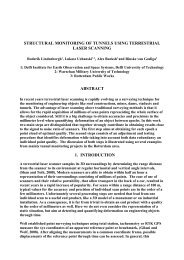
Geostatistics for Earth ObservationLecture 8, April 13, 2005Roderik Lindenbergh and Ramon Hanssen1DEOS, Mathematical Geodesy and PositioningDelft University of Technology

OverviewHandling spatial components. .• Short remark on anisotropy.• Spatial components.• Signal and covariance decomposition.• Range of influence.• Filter method.• Filter example.2DEOS, Mathematical Geodesy and Positioning

Anisotropy revisited.Let h = (x 1 , y 1 ) − (x 2 , y 2 ), that is, h ∈ IR 2 .1D method.• Determine geometric transformation A : IR 2 → IR 2 that convertsiso-variability ellipses into circles.• Use a 1D variogram on the transformed difference vectors, that is considerh→√h∗ · A · h → γ 1D ( √ h ∗ · A · h)2D method.“• Determine a base B = (iso-variability ellipses.uxuy” “,• Express h with respect to B, resulting in h ′ .vxvy”) for the principal axes of the• Use a 2D variogram γ 2D on h ′ = (h ′ x, h ′ y), so considerh → h ′ = B −1 · h → γ 2D (h ′ )3DEOS, Mathematical Geodesy and Positioning

Spatial components.Until now: one scale of spatialvariability modelled by onevariogram.But typically:Signal=Measurement inaccuracy+Short range signal+Long range signal4DEOS, Mathematical Geodesy and Positioning

Signal and covariance decomposition.Signal decomposition:Nested covariance model:H(p) = H 0 (p) + H 1 (p) + H 2 (p), p ∈ IR 2Cov(h) = Cov0(h) + Cov1(h) + Cov2(h),with ranges R 0 = 0 (nugget) and 0 < R 1 < R 2 .h ∈ IRWrite S = {p 1 , . . . , p n } for the observation locations.Consider the distance d(p 0 , S) between the estimation location p 0closest observation from S.and the5DEOS, Mathematical Geodesy and Positioning

Only far away observations: d(p 0 , S) > R 2 .Proximity vector vanishes:d n =0B@Cov 10.Cov n011 0CA = B@Cov0 10.Cov0 n011 0CA + B@Cov1 10.Cov1 n011 0CA + B@Cov2 10.Cov2 n011 0CA = B@0.011CA6DEOS, Mathematical Geodesy and Positioning

No close observations: R 1 < d(p 0 , S) < R 2 .Nugget and short range covariance vector have no influence in proximityvector:d n =0B@Cov 10.Cov n011 0CA = B@Cov0 10.Cov0 n011 0CA + B@Cov1 10.Cov1 n011 0CA + B@Cov2 10.Cov2 n011 0CA = B@Cov2 10.Cov2 n011CA7DEOS, Mathematical Geodesy and Positioning

Close observations: 0 < d(p 0 , S) < R 1 .Nugget has no influence in proximity vector:d n =0B@Cov 10..Cov n01 0CA = B@Cov0 10..Cov0 n01 0CA + B@Cov1 10..Cov1 n01 0CA + B@Cov2 10..Cov2 n01 0CA = B@Cov1 10..Cov1 n01 0CA + B@Cov2 10..Cov2 n01CA1111118DEOS, Mathematical Geodesy and Positioning

Coincidence with observation: d(p 0 , S) = 0.Ordinary Kriging just returns observation and ‘does not interpolate’.Apply this analysis to filter spatial components!DEOS, Mathematical Geodesy and Positioning9

FilteringWish list:• Avoid peaks at observation locations;• Smoothen short range variations;• Or, on the contrary, remove a long range trend.Method:• Filter one or more spatial components (like nugget effect, short or longrange variability) from the signal.• Combine results.How:• Omit the correponding covariance contribution(s) from the proximityvector.• Combine by e.g. subtracting the filtered interpolation from the OKinterpolation.10DEOS, Mathematical Geodesy and Positioning

Some filter results11DEOS, Mathematical Geodesy and Positioning