Adaptive Shadow Maps - Cornell Program of Computer Graphics
Adaptive Shadow Maps - Cornell Program of Computer Graphics
Adaptive Shadow Maps - Cornell Program of Computer Graphics

Create successful ePaper yourself
Turn your PDF publications into a flip-book with our unique Google optimized e-Paper software.
<strong>Adaptive</strong> <strong>Shadow</strong> <strong>Maps</strong><br />
Randima Fernando Sebastian Fernandez Kavita Bala Donald P. Greenberg ∗<br />
<strong>Program</strong> <strong>of</strong> <strong>Computer</strong> <strong>Graphics</strong><br />
<strong>Cornell</strong> University<br />
Abstract<br />
<strong>Shadow</strong> maps provide a fast and convenient method <strong>of</strong> identifying<br />
shadows in scenes but can introduce aliasing. This paper introduces<br />
the <strong>Adaptive</strong> <strong>Shadow</strong> Map (ASM) as a solution to this problem. An<br />
ASM removes aliasing by resolving pixel size mismatches between<br />
the eye view and the light source view. It achieves this goal by storing<br />
the light source view (i.e., the shadow map for the light source)<br />
as a hierarchical grid structure as opposed to the conventional flat<br />
structure. As pixels are transformed from the eye view to the light<br />
source view, the ASM is refined to create higher-resolution pieces<br />
<strong>of</strong> the shadow map when needed. This is done by evaluating the<br />
contributions <strong>of</strong> shadow map pixels to the overall image quality.<br />
The improvement process is view-driven, progressive, and confined<br />
to a user-specifiable memory footprint. We show that ASMs enable<br />
dramatic improvements in shadow quality while maintaining interactive<br />
rates.<br />
CR Categories: I.3.7 [<strong>Computer</strong> <strong>Graphics</strong>]: Three-Dimensional<br />
<strong>Graphics</strong> and Realism—Shading,<strong>Shadow</strong>ing;<br />
Keywords: Rendering, <strong>Shadow</strong> Algorithms<br />
1 Introduction<br />
<strong>Shadow</strong>s provide important information about the spatial relationships<br />
among objects [8]. One commonly used technique for shadow<br />
generation is the shadow map [9]. A shadow map is a depth image<br />
generated from the light source view. When rendering, points in<br />
the eye view are transformed into the light source view. The depths<br />
<strong>of</strong> the transformed points are then compared with the depths in the<br />
shadow map to determine if the transformed points are visible from<br />
the light source. A transformed point is considered lit if it is closer<br />
to the light than the corresponding point in the shadow map. Otherwise,<br />
the point is considered to be in shadow. This information is<br />
then used to shade the eye view image.<br />
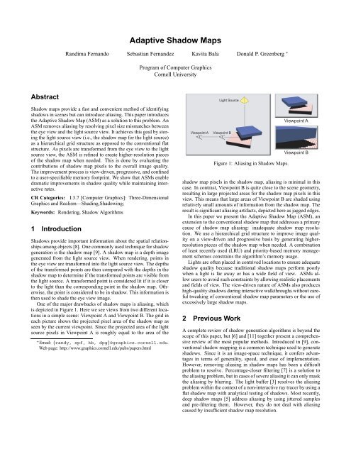
One <strong>of</strong> the major drawbacks <strong>of</strong> shadow maps is aliasing, which<br />
is depicted in Figure 1. Here we see views from two different locations<br />
in a simple scene: Viewpoint A and Viewpoint B. The grid in<br />
each picture shows the projected pixel area <strong>of</strong> the shadow map as<br />
seen by the current viewpoint. Since the projected area <strong>of</strong> the light<br />
source pixels in Viewpoint A is roughly equal to the area <strong>of</strong> the<br />
∗ Email: {randy, spf, kb, dpg}@graphics.cornell.edu.<br />
Web page: http://www.graphics.cornell.edu/pubs/papers.html<br />
Viewpoint A<br />
Light Source<br />
Viewpoint B<br />
Figure 1: Aliasing in <strong>Shadow</strong> <strong>Maps</strong>.<br />
Viewpoint A<br />
Viewpoint B<br />
shadow map pixels in the shadow map, aliasing is minimal in this<br />
case. In contrast, Viewpoint B is quite close to the scene geometry,<br />
resulting in large projected areas for the shadow map pixels in this<br />
view. This means that large areas <strong>of</strong> Viewpoint B are shaded using<br />
relatively small amounts <strong>of</strong> information from the shadow map. The<br />
result is significant aliasing artifacts, depicted here as jagged edges.<br />
In this paper we present the <strong>Adaptive</strong> <strong>Shadow</strong> Map (ASM), an<br />
extension to the conventional shadow map that addresses a primary<br />
cause <strong>of</strong> shadow map aliasing: inadequate shadow map resolution.<br />
We use a hierarchical grid structure to improve image quality<br />
on a view-driven and progressive basis by generating higherresolution<br />
pieces <strong>of</strong> the shadow map when needed. A combination<br />
<strong>of</strong> least recently used (LRU) and priority-based memory management<br />
schemes constrains the algorithm’s memory usage.<br />
Lights are <strong>of</strong>ten placed in contrived locations to ensure adequate<br />
shadow quality because traditional shadow maps perform poorly<br />
when a light is far away or has a wide field <strong>of</strong> view. ASMs allow<br />
users to avoid such constraints by allowing realistic placements<br />
and fields <strong>of</strong> view. The view-driven nature <strong>of</strong> ASMs also produces<br />
high-quality shadows during interactive walkthroughs without careful<br />
tweaking <strong>of</strong> conventional shadow map parameters or the use <strong>of</strong><br />
excessively large shadow maps.<br />
2 Previous Work<br />
A complete review <strong>of</strong> shadow generation algorithms is beyond the<br />
scope <strong>of</strong> this paper, but [6] and [11] together present a comprehensive<br />
review <strong>of</strong> the most popular methods. Introduced in [9], conventional<br />
shadow mapping is a common technique used to generate<br />
shadows. Since it is an image-space technique, it confers advantages<br />
in terms <strong>of</strong> generality, speed, and ease <strong>of</strong> implementation.<br />
However, removing aliasing in shadow maps has been a difficult<br />
problem to resolve. Percentage-closer filtering [7] is a solution to<br />
the aliasing problem, but in cases <strong>of</strong> severe aliasing it can only mask<br />
the aliasing by blurring. The light buffer [3] resolves the aliasing<br />
problem within the context <strong>of</strong> a non-interactive ray tracer by using a<br />
flat shadow map with analytical testing <strong>of</strong> shadows. Most recently,<br />
deep shadow maps [5] address aliasing by using jittered samples<br />
and pre-filtering them. However, they do not deal with aliasing<br />
caused by insufficient shadow map resolution.
3 The <strong>Adaptive</strong> <strong>Shadow</strong> Map<br />
ASMs are based on the observation that a high-quality shadow map<br />
need not be <strong>of</strong> uniform high resolution; only regions that contain<br />
shadow boundaries need to be sampled densely. In those regions,<br />
the resolution <strong>of</strong> the shadow map should be at least as high as the<br />
corresponding region in the eye view to avoid aliasing artifacts.<br />
An ASM hierarchically subdivides an ordinary shadow map,<br />
providing higher resolutions in visually important regions. Like<br />
a conventional shadow map, an ASM takes as input a set <strong>of</strong> transformed<br />
eye view points and allows shadow queries on this set, returning<br />
true if a particular point is lit and false otherwise. In s<strong>of</strong>tware<br />
systems, ASMs can seamlessly replace conventional shadow<br />
maps.<br />
An ASM has three main characteristics:<br />
• It is view-driven, meaning that the hierarchical grid structure<br />
is updated based on the user’s viewpoint.<br />
• It is confined to a user-specifiable memory limit. Memory is<br />
managed efficiently and the ASM avoids the explosive growth<br />
in memory usage that would be required by a conventional<br />
shadow map <strong>of</strong> the same visual quality.<br />
• It is progressive, meaning that once a particular viewpoint is<br />
established, image quality continues to improve until the userprescribed<br />
memory limit is reached.<br />
ASMs are organized as trees. Each node in an ASM tree has a<br />
shadow map <strong>of</strong> a fixed resolution and a partitioning <strong>of</strong> that shadow<br />
map into a fixed number <strong>of</strong> cells. Each <strong>of</strong> these cells may contain<br />
another tree node. Two operations may be performed on a cell in<br />
the tree. An empty cell may have a new node assigned to it when<br />
it is determined that the resolution <strong>of</strong> the shadow map region corresponding<br />
to the cell is not high enough to provide the required<br />
image quality. A cell containing a node may also have that node<br />
and its descendants deleted. This is done in response to the userspecified<br />
restrictions on memory usage.<br />
3.1 Creating Nodes<br />
At any time there are many cells that require new nodes to be assigned<br />
to them. In an interactive application, it is not always possible<br />
to fulfill all <strong>of</strong> these requirements. Therefore, we use a costbenefit<br />
metric to determine which cells to satisfy. It is only beneficial<br />
to create a new node (and hence a higher resolution shadow<br />
map piece) if it causes a perceived improvement in shadow quality.<br />
We quantify this perceived benefit by counting the number <strong>of</strong> transformed<br />
eye pixels within the cell that straddle a depth discontinuity<br />
and whose shadow map resolution is lower than the eye view resolution.<br />
We use the mip-mapping capability <strong>of</strong> commodity graphics<br />
hardware to estimate the resolution in the eye view and in the<br />
shadow map. Section 4.1 explains this in detail.<br />
The cost <strong>of</strong> creating a new node is the amount <strong>of</strong> time required<br />
to generate its new shadow map. Using the ratio <strong>of</strong> eye view pixel<br />
size to shadow map pixel size, the resolution required for the new<br />
shadow map to match the eye view resolution is:<br />
Eye V iew P ixel P rojected Area<br />
N required = N current<br />
<strong>Shadow</strong> Map P ixel P rojected Area<br />
where N is the number <strong>of</strong> pixels in a shadow map cell.<br />
The cost <strong>of</strong> generating a new shadow map can be approximated<br />
by:<br />
cost = aN required + b<br />
This cost model is based on the fact that hardware read-back performance<br />
varies roughly linearly with the size <strong>of</strong> the buffer being read<br />
back, becoming increasingly inefficient as the read-back size gets<br />
very small. We perform a calibration test as a preprocess to evaluate<br />
a (the per-pixel rendering cost) and b (the constant overhead) for a<br />
given hardware setup.<br />
The benefit <strong>of</strong> a new shadow map is the number <strong>of</strong> resolutionmismatched<br />
eye pixels that could be resolved. Once the cost-benefit<br />
ratio is computed for all prospective cells, the cells are sorted according<br />
to this ratio. To maintain consistent frame rates, new<br />
shadow map nodes are only generated for the most pr<strong>of</strong>itable cells<br />
from this list until a given time limit has passed.<br />
3.2 Removing Nodes<br />
Since the ASM only uses a fixed amount <strong>of</strong> memory, a particular<br />
node’s memory might need to be reclaimed. In order to do so, we<br />
use a LRU scheme on all nodes that were not used in the last frame,<br />
removing the least recently used nodes. If there are no such nodes,<br />
then all nodes are currently visible. In this case, we remove an<br />
existing node only if a new node that needs to be created has a<br />
greater benefit than the existing node.<br />
4 Implementation<br />
This section discusses additional techniques and optimizations.<br />
4.1 Mip-mapping<br />
To determine when resolution mismatches occur, the algorithm<br />
must calculate the projected area <strong>of</strong> a pixel (i.e., the area that the<br />
pixel covers in world-space). Performing this calculation in s<strong>of</strong>tware<br />
would be too expensive for interactive rates, so we approximate<br />
this calculation using mip-mapping.<br />
Mip-mapping [10] is traditionally used to avoid aliasing artifacts<br />
associated with texture-mapping. Current graphics hardware implements<br />
perspective-correct mip-mapping, which interpolates between<br />
textures <strong>of</strong> different resolutions based on the projected area<br />
<strong>of</strong> the pixels being rendered. We use this feature to quickly approximate<br />
the projected pixel area as follows: the algorithm places<br />
the resolution <strong>of</strong> each mip-map level in all the texels <strong>of</strong> that level.<br />
Thus, the smallest level has a 1 in every texel, the second smallest<br />
level has a 2, the third smallest level has a 4, and so on. Texture<br />
coordinates are set up so that world-space texel sizes are uniform.<br />
Every polygon is then drawn with this mip-mapped texture. When<br />
the frame is read back, each pixel contains its trilinearly interpolated<br />
mip-map level, which is a reasonable approximation <strong>of</strong> its<br />
projected area. Anisotropic filtering is used to improve the accuracy<br />
<strong>of</strong> the approximation.<br />
As a further optimization, the mip-map level is encoded only<br />
in the alpha channel while the rest <strong>of</strong> the mip-map is white. This<br />
allows the read-back to be done simultaneously with the polygon ID<br />
read-backs described below, eliminating an extra rendering pass.<br />
4.2 Combining ID and Depth Comparisons<br />
Conventional shadow maps commonly use a depth comparison with<br />
a bias factor to check if transformed pixels are lit. However, this approach<br />
exhibits artifacts on surfaces near edge-on to the light and<br />
has difficulties in scenes with varying geometric scale. Using perpolygon<br />
IDs to determine visibility instead <strong>of</strong> depth comparisons<br />
was proposed in [4]. This approach is better in many cases but<br />
results in artifacts along mesh boundaries. Therefore, we use a<br />
combination <strong>of</strong> per-polygon IDs and depth comparisons to perform<br />
the visibility determination for transformed pixels. If the ID test
fails, the conventional depth comparison allows us to avoid artifacts<br />
along polygon boundaries. Our results show that this simple modification<br />
is more robust than using just per-polygon IDs or depth<br />
comparisons, although the bias problem persists.<br />
4.3 Optimizations<br />
It is possible to accelerate ASM queries using a depth culling technique<br />
similar to that described in [2]. A cache storing the most<br />
recently queried leaf node further accelerates ASM lookups. Lowlevel<br />
optimizations such as using Pentium family SSE/SSE2 instructions<br />
could be used to speed up pixel reprojection from the<br />
eye view to the shadow map.<br />
Our approach requires frequent renderings and read-backs as<br />
cells are refined. Since it is inefficient to redraw the whole scene<br />
for each grid cell during refinement, we use frustum culling for<br />
each cell in the topmost level <strong>of</strong> the hierarchy.<br />
Since analysis <strong>of</strong> all pixels in the image can be expensive, our<br />
algorithm performs the cost-benefit analysis only on a fraction <strong>of</strong><br />
the transformed pixels. This choice might result in slower convergence<br />
to an accurate solution. However, in our implementation,<br />
we found that analyzing one-eighth <strong>of</strong> the pixels gives good performance<br />
without significantly affecting the rate <strong>of</strong> convergence.<br />
5 Results<br />
Figures 2, 3, and 4 present our results for an interactive walkthrough<br />
<strong>of</strong> a 31,000-polygon scene at an image resolution <strong>of</strong> 512×512 pixels.<br />
Our timings were performed on a 1 GHz Pentium III with a<br />
NVIDIA GeForce2 Ultra graphics board. The scene features three<br />
different objects designed to test different aspects <strong>of</strong> our algorithm.<br />
The light source is a point light with a 122 ◦ field <strong>of</strong> view. It is<br />
placed on the room ceiling, far from the objects. The first object<br />
is a 20,000-polygon bunny model, which illustrates the algorithm’s<br />
ability to deal with small triangles and frequent variations in polygon<br />
ID. The other two objects are a robot and a sculpture with a fine<br />
mesh, which demonstrate the algorithm’s ability to find and refine<br />
intricate shadow details <strong>of</strong> varying scale.<br />
During the walkthrough, a conventional 2,048×2,048 pixel<br />
shadow map (using 16 MB <strong>of</strong> storage with 32 bits <strong>of</strong> depth per<br />
pixel) averaged 8.5 frames per second, while our algorithm (also<br />
using 16 MB <strong>of</strong> memory) averaged 4.9 frames per second. Figures<br />
2 and 3 illustrate the dramatic improvement in image quality<br />
achieved by the ASM. For close-ups <strong>of</strong> objects, the equivalent conventional<br />
shadow map size is very large (65,536×65,536 pixels in<br />
Figure 2 and 524,288×524,288 pixels in Figure 3). Creating such a<br />
shadow map in practice for an interactive application would be infeasible<br />
not only because <strong>of</strong> the long creation time, but also because<br />
<strong>of</strong> the enormous storage requirements.<br />
Our results also demonstrate the ASM’s ability to accommodate<br />
a wide field <strong>of</strong> view. Because <strong>of</strong> the ASM’s view-driven nature,<br />
the starting shadow map size can be relatively small and its field<br />
<strong>of</strong> view can be relatively large. In our walkthrough, the starting<br />
resolution <strong>of</strong> the ASM was 512×512 pixels.<br />
Figure 4 illustrates the algorithm’s memory management. From<br />
left to right, we show images generated with a 2,048×2,048 pixel<br />
conventional shadow map, an ASM using 8 MB <strong>of</strong> memory, and<br />
an ASM using 16 MB <strong>of</strong> memory. The differences between the two<br />
ASM images are small, but both show considerable improvement in<br />
image quality when compared to the image on the left. To highlight<br />
the improvement in image quality from an 8 MB ASM to a 16 MB<br />
ASM, we have magnified two sections <strong>of</strong> each image.<br />
The ASM used approximately 203 ms per frame, while a conventional<br />
2,048×2,048 pixel shadow map used 117 ms for the same<br />
total memory usage (16 MB). The extra time was spent on costbenefit<br />
analysis (30 ms), node creation (5 ms), traversals through<br />
the hierarchy for queries (35 ms), and an extra rendering and readback<br />
<strong>of</strong> the scene to gather per-polygon ID information (16 ms).<br />
6 Conclusions<br />
This paper presents a new technique, the ASM, which uses adaptive<br />
subdivision to address aliasing in shadow maps caused by insufficient<br />
shadow map resolution. ASMs are view-driven, progressive,<br />
and run in a user-specifiable memory footprint. They interface with<br />
applications in the same way as conventional shadow maps, allowing<br />
them to be easily integrated into existing programs that use s<strong>of</strong>tware<br />
shadow mapping. Since ASMs automatically adapt to produce<br />
high-quality images and do not require experienced user intervention,<br />
they should be useful in interactive modeling applications and<br />
in <strong>of</strong>f-line renderers.<br />
The algorithm presented in this paper can be extended to prefilter<br />
and compress refined shadow map cells using techniques described<br />
in [5]. In addition, perceptual masking [1] can be used to<br />
refine less in heavily masked areas.<br />
7 Acknowledgements<br />
We would like to thank Bruce Walter, Eric Haines, Parag Tole,<br />
Fabio Pellacini, and Reynald Dumont for their insights and comments,<br />
Linda Stephenson for her administrative assistance, and<br />
Rich Levy for his help in making the video. We would also like to<br />
thank the anonymous reviewers for their valuable comments. This<br />
work was supported in part by the National Science Foundation Science<br />
and Technology Center for <strong>Computer</strong> <strong>Graphics</strong> and Scientific<br />
Visualization (ASC-8920219). We also gratefully acknowledge the<br />
generous support <strong>of</strong> the Intel Corporation and the NVIDIA Corporation.<br />
References<br />
[1] J. A. Ferwerda, S. N. Pattanaik, P. Shirley, and D. P. Greenberg. A Model <strong>of</strong> Visual<br />
Masking for <strong>Computer</strong> <strong>Graphics</strong>. In Proceedings <strong>of</strong> SIGGRAPH 97, <strong>Computer</strong><br />
<strong>Graphics</strong> Proceedings, Annual Conference Series, pages 143–152, August<br />
1997. T. Whitted, editor.<br />
[2] N. Greene and M. Kass. Hierarchical Z-Buffer Visibility. In Proceedings <strong>of</strong> SIG-<br />
GRAPH 93, <strong>Computer</strong> <strong>Graphics</strong> Proceedings, Annual Conference Series, pages<br />
231–240, August 1993. J. T. Kajiya, editor.<br />
[3] E. A. Haines and D. P. Greenberg. The Light Buffer: a <strong>Shadow</strong> Testing Accelerator.<br />
IEEE <strong>Computer</strong> <strong>Graphics</strong> and Applications, 6(9):6–16, September 1986.<br />
[4] J. C. Hourcade and A. Nicolas. Algorithms for Antialiased Cast <strong>Shadow</strong>s. <strong>Computer</strong><br />
and <strong>Graphics</strong>, 9(3):259–265, 1985.<br />
[5] T. Lokovic and E. Veach. Deep <strong>Shadow</strong> <strong>Maps</strong>. In Proceedings <strong>of</strong> SIGGRAPH<br />
2000, <strong>Computer</strong> <strong>Graphics</strong> Proceedings, Annual Conference Series, pages 385–<br />
392, July 2000. K. Akeley, editor.<br />
[6] T. Möller and E. A. Haines. Real-Time Rendering. A. K. Peters, Massachusetts,<br />
1999.<br />
[7] W. T. Reeves, D. H. Salesin, and R. L. Cook. Rendering Antialiased <strong>Shadow</strong>s<br />
with Depth <strong>Maps</strong>. <strong>Computer</strong> <strong>Graphics</strong> (Proceedings <strong>of</strong> SIGGRAPH 87),<br />
21(4):283–291, July 1987. M. C. Stone, editor.<br />
[8] L. R. Wanger, J. A. Ferwerda, and D. P. Greenberg. Perceiving Spatial Relationships<br />
in <strong>Computer</strong>-Generated Images. IEEE <strong>Computer</strong> <strong>Graphics</strong> and Applications,<br />
12(3):44–58, May 1992.<br />
[9] L. Williams. Casting Curved <strong>Shadow</strong>s on Curved Surfaces. <strong>Computer</strong> <strong>Graphics</strong><br />
(Proceedings <strong>of</strong> SIGGRAPH 78), 12(3):270–274, August 1978. R. L. Phillips,<br />
editor.<br />
[10] L. Williams. Pyramidal Parametrics. <strong>Computer</strong> <strong>Graphics</strong> (Proceedings <strong>of</strong> SIG-<br />
GRAPH 83), 17(3):1–11, July 1983. P. Tanner, editor.<br />
[11] A. Woo, P. Poulin, and A. Fournier. A Survey <strong>of</strong> <strong>Shadow</strong> Algorithms. IEEE<br />
<strong>Computer</strong> <strong>Graphics</strong> and Applications, 10(6):13–32, November 1990.
Figure 2: A conventional 2,048×2,048 pixel shadow map (left) compared to a 16 MB ASM (right).<br />
EFFECTIVE SHADOW MAP SIZE: 65,536×65,536 PIXELS.<br />
Figure 3: A conventional 2,048×2,048 pixel shadow map (left) compared to a 16 MB ASM (right).<br />
EFFECTIVE SHADOW MAP SIZE: 524,288×524,288 PIXELS.<br />
Figure 4: A conventional 2048×2048 pixel shadow map (left), an 8 MB ASM (center), and a 16 MB ASM (right).