Tunneling

Chemistry 460
Spring 2013
Dr. Jean M. Standard
February 5, 2013
Tunneling
Definition of Tunneling
Tunneling is defined to be penetration of the wavefunction into a classically forbidden region. Since the
wavefunction is non-zero in the classically forbidden region, the probability density ψ *ψ also is non-zero; thus,
there is a finite probability that the particle will exist in a region that it could never be in if it were obeying classical
mechanics. In this situation, we say that the particle has tunneled into the classically forbidden region. [A region is
said to be classically forbidden if the particle’s energy is less than the potential energy in the region, E < V .]
€
Example 1: Half-Infinite Well
€
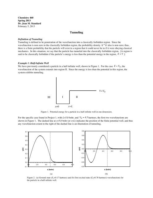
We have previously considered a particle in a half-infinite well, shown in Figure 1. For the case E < V 0 , the
wavefunction of the system extends into region II. Since the energy is less than the potential in this region, the
system exhibits tunneling.
€
III I II
V=V 0
x=0 x=L
Figure 1. Potential energy for a particle in a half-infinite well in one dimension.
For the specific case found in Project 1, with L=5.0 bohr, and V 0 = 4.5 hartrees, the first two wavefunctions are
shown in Figure 1. The dashed line at x=5.0 bohr (or x=L) indicates the position of the finite potential well, and thus
any wavefunction extent to the right of the dashed line is an illustration of tunneling.
0.7
€
0.8
0.6
0.6
0.5
0.4
0.4
0.2
ψ(x)
0.3
0.2
ψ(x)
0.0
0.0 2.0 4.0 6.0 8.0 10.0
-0.2
0.1
-0.4
0.0
0.0 2.0 4.0 6.0 8.0 10.0
-0.1
x (bohr)
-0.6
-0.8
x (bohr)
(a) (b)
Figure 2. (a) Ground state (E 1 =0.17 hartrees) and (b) first excited state (E 2 =0.70 hartrees) wavefunctions for
the particle in a half-infinite well.

2
For energies closer to the top of the well, the tunneling proportion increases. Shown in Figure 3 are the
wavefunctions corresponding to the fourth and fifth energy levels for this system.
0.8
0.8
0.6
0.6
0.4
0.4
0.2
0.2
ψ(x)
0.0
0.0 2.0 4.0 6.0 8.0 10.0
-0.2
ψ(x)
0.0
0.0 2.0 4.0 6.0 8.0 10.0
-0.2
-0.4
-0.4
-0.6
-0.6
-0.8
-0.8
x (bohr)
x (bohr)
(a) (b)
Figure 3. (a) Third excited state (E 4 =2.75 hartrees) and (b) fourth excited state (E 5 =4.16 hartrees)
wavefunctions for the particle in a half-infinite well.
Notice that for the fourth excited state, with an energy very close to the top of the barrier (E 5 =4.16 hartrees
compared to a barrier of 4.5 hartrees), the tunneling is substantial. For this system, we can determine the tunneling
probability by integrating the probability density from x=L to x= ∞. For the 1 st energy level the tunneling probability
is 0.0025, while for the 5 th energy level the tunneling probability is 0.18.
€
Example 2: Tunneling Through a Barrier of Finite Width
Another simple example of tunneling is the case of a barrier of finite width, illustrated in Figure 4.
V=V 0
I II III
x=0 x=L
Figure 4. Potential energy for a particle interacting with a finite barrier in one dimension.
The potential energy of the system may be described by the following equation,
V (x) =
⎧⎧ 0,
⎪⎪
⎨⎨ V 0 ,
⎪⎪
⎩⎩ 0,
x < 0
0 ≤ x ≤ L
x > L
⎫⎫
⎪⎪
⎬⎬ .
⎪⎪
⎭⎭
The method of solution is similar to what we did for the particle in a half-infinite well. However, there are two
degenerate solutions, one in which the particle is initially traveling to the right and one in which the particle is
€
initially traveling to the left. Only one of these degenerate cases needs to be considered. Here, we will assume that
the particle is traveling to the right, so it is initially incident on the barrier from region I.

3
For the case
E < V 0 , the general solutions may be given as
€
ψ I ( x) = A e ik1x + Be −ik 1x
ψ II ( x) = C e k2x + De −k 2x
ψ III ( x) = F e ik 1 x .
The wave vectors
k 1 and
k 2 are defined as
€
€
€
k 1 =
2mE
and k 2 =
2m ( V 0 − E)
.
In region I, and in general for unbounded regions where the potential energy is zero, we use exponentials with
imaginary exponents as the preferred form of the wavefunction. The two parts of the wavefunction written in this
€
form can be related to waves traveling in the positive and negative x directions, respectively.
Notice that in region II, we have used exponentials with real rather than imaginary exponents. This is the preferred
form in regions where the total energy E is less than the potential energy V 0 .
Also notice that in region III, there is no wave traveling to the left. This is because we started with a wave traveling
to the right, and in region III, no wave traveling to the left can form because there is nothing for the wave to reflect
€
from.
Matching the wavefunctions and their first derivatives at the boundaries x=0 and x=L yields conditions among the
arbitrary constants A, B, C, D, and F. Of particular interest is a quantity called the transmission coefficient T. The
transmission coefficient T is related to the ratio of the probability density current that is transmitted through the
barrier to the incident probability density current. The probability density current S is defined as
S = v ψ *ψ ,
where v is the particle velocity. Thus, the transmission coefficient T is
€
T = S tr
S in
,
€
where S tr is the transmitted probability density current and S in is the incident probability density current. For the
specific case here, the transmitted wave in region € III has the form Fe i k 1x . Since this form has a momentum
eigenvalue given by k 1 , the velocity is
€
v € tr = p tr
m = k 1
m .
€
Similarly, the incident wave in region I has the form
k 1 , the velocity is
€
Ae i k 1x . Since this form has a momentum eigenvalue given by
€
€
v in = p in
m = k 1
m .
€

4
Substituting, we can calculate the transmission coefficient T,
T = S tr
S in
= v trψ * tr ψ tr
v in ψ * in ψ in
=
T = F A
k 1
m F * e−ik 1x Fe
ik 1 x
k 1
m A * e−ik 1 x Ae ik 1 x
2
.
Using the relations obtained from matching the wavefunctions and first derivatives at the boundaries, the ratio of
F/A may be determined. For this system, the transmission coefficient is
€
T = F A
2
,
or T =
1 +
1
sinh 2 .
( k 2 L)
4E ⎛⎛
1 − E ⎞⎞
⎜⎜ ⎟⎟
V 0 ⎝⎝ V 0 ⎠⎠
In this equation, the function sinh is the hyperbolic sine function. It is defined
€
sinhbx = ebx − e −bx
.
2
Though not appearing in this expression, the hyperbolic cosine function, cosh, is defined in a similar fashion,
€
coshbx = ebx + e −bx
.
2
For values of the energy less than V 0 , the transmission coefficient only gets large for energies close to the top of the
barrier, as illustrated in Figure 5.
€
€
0.020
0.018
T
0.016
0.014
0.012
0.010
0.008
0.006
0.004
0.002
0.000
0.0 0.2 0.4 0.6 0.8 1.0 1.2
E/V 0
Figure 5. Transmission coefficient for a particle tunneling through a finite barrier in one dimension.

5
Example 3: Double Well Potential
A common model that is used to represent inversion in molecules like ammonia is the double well potential shown
in Figure 6.
V=V 0
L
x=0
x=a x=c x=d
Figure 6. Double well potential.
This potential mimics the inversion of ammonia through its planar form, illustrated in Figure 7.
(a)
(b)
Figure 7. (a) Inversion motion of ammonia through the planar transition state. (b) Potential energy of
inversion of ammonia as a function of the out-of-plane angle.
Classically, the ammonia molecule in its ground state does not have enough energy to go over the barrier.
Therefore, a classical ammonia molecule would not experience inversion. In quantum mechanics, though, the
ammonia molecule experiences tunneling through the barrier and so undergoes inversion.