Derivation of Backpropagation

Derivation of Backpropagation
1 Introduction
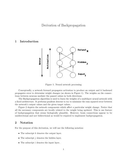
Figure 1: Neural network processing
Conceptually, a network forward propagates activation to produce an output and it backward
propagates error to determine weight changes (as shown in Figure 1). The weights on the connections
between neurons mediate the passed values in both directions.
The Backpropagation algorithm is used to learn the weights of a multilayer neural network with
a fixed architecture. It performs gradient descent to try to minimize the sum squared error between
the network’s output values and the given target values.
Figure 2 depicts the network components which affect a particular weight change. Notice that
all the necessary components are locally related to the weight being updated. This is one feature
of backpropagation that seems biologically plausible. However, brain connections appear to be
unidirectional and not bidirectional as would be required to implement backpropagation.
2 Notation
For the purpose of this derivation, we will use the following notation:
• The subscript k denotes the output layer.
• The subscript j denotes the hidden layer.
• The subscript i denotes the input layer.
1

Figure 2: The change to a hidden to output weight depends on error (depicted as a lined pattern)
at the output node and activation (depicted as a solid pattern) at the hidden node. While the
change to a input to hidden weight depends on error at the hidden node (which in turn depends
on error at all the output nodes) and activation at the input node.
• w kj denotes a weight from the hidden to the output layer.
• w ji denotes a weight from the input to the hidden layer.
• a denotes an activation value.
• t denotes a target value.
• net denotes the net input.
3 Review of Calculus Rules
d(e u )
dx = eudu dx
d(g + h)
dx
= dg
dx + dh
dx
d(g n )
dx
dg
= ngn−1
dx
4 Gradient Descent on Error
We can motivate the backpropagation learning algorithm as gradient descent on sum-squared error
(we square the error because we are interested in its magnitude, not its sign). The total error in a
network is given by the following equation (the 1 2
will simplify things later).
E = 1 ∑
(t k − a k ) 2
2
k
We want to adjust the network’s weights to reduce this overall error.
∆W ∝ − ∂E
∂W
We will begin at the output layer with a particular weight.
2

∆w kj ∝ − ∂E
∂w kj
However error is not directly a function of a weight. We expand this as follows.
∆w kj = −ε ∂E ∂a k ∂net k
∂a k ∂net k ∂w kj
Let’s consider each of these partial derivatives in turn. Note that only one term of the E summation
will have a non-zero derivative: the one associated with the particular weight we are considering.
4.1 Derivative of the error with respect to the activation
Now we see why the 1 2
∂E
= ∂(1 2 (t k − a k ) 2 )
= −(t k − a k )
∂a k ∂a k
in the E term was useful.
4.2 Derivative of the activation with respect to the net input
∂a k
= ∂(1 + e−net k) −1
=
∂net k ∂net k
e −net k
(1 + e −net k ) 2
We’d like to be able to rewrite this result in terms of the activation function. Notice that:
1
1 −
1 + e −net = e−net k
k 1 + e −net k
Using this fact, we can rewrite the result of the partial derivative as:
a k (1 − a k )
4.3 Derivative of the net input with respect to a weight
Note that only one term of the net summation will have a non-zero derivative: again the one
associated with the particular weight we are considering.
∂net k
= ∂(w kja j )
= a j
∂w kj ∂w kj
4.4 Weight change rule for a hidden to output weight
Now substituting these results back into our original equation we have:
δ k
{ }} {
∆w kj = ε(t k − a k )a k (1 − a k ) a j
Notice that this looks very similar to the Perceptron Training Rule. The only difference is the
inclusion of the derivative of the activation function. This equation is typically simplified as shown
below where the δ term repesents the product of the error with the derivative of the activation
function.
∆w kj = εδ k a j
3

4.5 Weight change rule for an input to hidden weight
Now we have to determine the appropriate weight change for an input to hidden weight. This is
more complicated because it depends on the error at all of the nodes this weighted connection can
lead to.
∆w ji ∝ −[ ∑ ∂E ∂a k ∂net k ∂a j ∂net j
]
∂a
k k ∂net k ∂a j ∂net j ∂w ji
= ε[ ∑ k
δ k
{ }} {
(t k − a k )a k (1 − a k )w kj ]a j (1 − a j )a i
δ j
{ }} {
= ε[ ∑ δ k w kj ]a j (1 − a j ) a i
k
∆w ji = εδ j a i
4