Using Excel for Linear Regression Calculations

Chemistry 215
Using Excel for Linear Regression Calculations
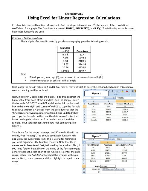
Excel contains several functions allow you to find the slope, intercept, and R 2 (the square of the correlation
coefficient) for a graph. The functions are named SLOPE(), INTERCEPT(), and RSQ(). The following example shows
how these functions are used
Example – Calibration Curve
The analysis of ethanol in wine by gas chromatography gave the following results:
Standard
(vol %) Peak Area
Blank 11.4
4.99 1240.3
9.98 2489.1
14.97 3741.4
20.96 4976.0
Sample 2849.7
Find:
• The slope (m), intercept (b), and square of the correlation coeff. (R 2 )
• The concentration of ethanol in the sample
First, enter the data in columns A and B. You may or may not wish to enter the column headings; in this example
column headings will be included.
Figure 1
Next, in column C correct for the blank. To do this, subtract the
blank value from each of the standards and the sample. Enter
the formula “=B2‐B$2” in cell C2 and double‐click on the small
box in the lower right and corner of cell C2 to copy the formula
to cells C3 through C7. (Recall from the Excel tutorial that the
“$” character prevents a reference from being updated when
you copy the formula. In this case the data in row 2 – i.e. the
blank reading – is subtracted from each standard and the
sample.) Your spreadsheet should now look something like
Figure 1.
Type labels for the slope, intercept, and R 2 in cells A9‐A11. In
cell B9, type “=slope(”. You should see Excel’s function help
pop up by the cursor (Figure 2). This is useful for reminding
you what arguments the function requires. Note that the y
values are to be entered first, followed by the x values. Also, if
you need further help, click on the name of the function to get
a more thorough description of the function. To enter the data
range, either type “A3:A6” or highlight the y values with your
cursor. Next, type a comma and then highlight or type in the x
range.
Figure 2

Figure 3 shows what the screen should look like after entering the x and y ranges. Note that the ranges are colorcoded.
Press ENTER to calculate the slope. (Typing the closing parenthesis is optional; Excel will assume you want
to close the parenthesis if you don’t type it.) Repeat this procedure for the intercept and R 2 . These functions are
INTERCEPT() and RSQ(), respectively, and both require that you enter the y range first. At this point you may wish
to adjust the number of decimal points in each cell.
The screen should now resemble Figure 4.
Figure 3
Figure 4
Finally, compute the concentration of the unknown by entering “=(C7‐B10)/B9” in cell D7 (Figure 5). Adjust the
number of decimal places as necessary.
Final Result!
Figure 5