Quantum Chemistry Exam 1 – Solutions

Chemistry 460
Spring 2013
Dr. Jean M. Standard
February 19, 2013
Quantum Chemistry Exam 1 – Solutions
1.) (16 points) Explain or provide an example illustrating each of the following concepts.
a.) Born probability interpretation
The Born probability interpretation states that the probability of finding a particle in the volume
dτ = dx dy dz between x, y, z x + dx, y + dy, z + dz
ψ * x, y,z
( ) and ( ) is given by
( ) ψ( x, y,z) dτ .
€
b.) Normalization €
€
€
Normalization refers to the scaling of a wavefunction so that the total probability "sums" to 1. Since the
wavefunction is expressed in terms of continuous variables, the sum becomes an integral, and the
normalization requirement is
∫ ψ * ψ dτ = 1 ,
and the integral is over all space.
€
c.) Orthogonal functions
Two functions f and g are said to be orthogonal if the integral of their product (with one function as the
complex conjugate) equals 0,
∫ f * g dτ = 0 .
d.) Tunneling
€
Tunneling is the penetration of the wavefunction into a classically forbidden region (i.e., a region in which
E < V ).
€

2.) (22 points) A system is in a state described by the wavefunction
of x from –∞ to +∞ . (k is a constant).
ψ(x) = e −ikx
for all values
2
a.) Show that this wavefunction is an eigenfunction of the € linear momentum operator for
the x coordinate. What is the eigenvalue
To show that the wavefunction is an eigenfunctions of the momentum operator, we must show that
€
ˆ p x ψ(x) = Pψ(x),
where P is a constant (the eigenvalue). For ψ(x) = e −i kx , application of the momentum operator gives
€
ˆ p x e −i kx = − i d dx (e−i kx )
ˆ p x ψ x
= i 2 −i kx
k e
( ) = − kψ( x) .
So, we see that the wavefunction ψ(x) =e −i kx is an eigenfunction of the momentum operator with
eigenvalue − k . €
€
€
b.) Determine how the energy eigenvalue E of the Schrödinger equation is related to the
constant k for this system if the potential energy equals 0 for all x.
To determine how E and k are related, the wavefunction can be substituted into the Schrödinger equation.
Since the potential energy is zero everywhere, the Schrödinger equation is
− 2
2m
d 2
dx 2 ψ x
( ) = Eψ x
( ).
Substituting the form
€
ψ(x) = e −ikx ,
€
− 2
2m
d 2
dx 2 e−ikx = E e −ikx .
Taking the second derivative on the left and simplifying yields
€
− 2
2m
{ − k 2 e −ikx } = E e −ikx
2 k 2
2m e−ikx = E e −ikx .
€

2 b.) continued
3
Since the function
€
e −i kx is the same on both sides, we can divide this out to give
2 k 2
2m = E .
Solving for the constant k,
€
k =
2mE
.
€

3.) (16 points) Consider two operators A ˆ and B ˆ which are Hermitian. Prove that their
product A ˆ B ˆ is Hermitian only if A ˆ and B ˆ commute; that is, only if A ˆ B ˆ = B ˆ A ˆ . Recall that
for an operator O ˆ to be Hermitian, it must satisfy the relation
€
€
€ €
∞
€ ψ * ( x) € O ˆ φ ( x
∞
∫ ) dx = O ˆ
∫ ψ( x)
( ) € dx ,
−∞
−∞
( ) * φ x
4
or in Dirac notation,
€
ψ
O ˆ φ = O ˆ ψ φ .
We must show that the product operator €
€
A ˆ B ˆ satisfies the Hermitian relation,
( ) * φ x
∞
ψ * ( x) ˆ
€
A B ˆ φ ( x
∞
∫ ) dx = A ˆ
∫ B ˆ ψ ( x ) ( ) dx .
−∞
−∞
To begin, we can start with the left side of the Hermitian relation,
∞
∫ ψ * ( x) A ˆ B ˆ φ ( x ) dx ,
−∞
and then manipulate it to try to produce the right side of the Hermitian relation. In the integral above, recall
that the operator nearest the function € operates first to produce a new function. Therefore, B ˆ operates on φ x
produce the new function B ˆ φ( x). Grouping terms, the integral above becomes
€
( ) dx
∞
ψ * ( x) A ˆ B ˆ
∫ φ ( x ) .
This looks like the left side of the Hermitian relation for the operator
Using the Hermitian character of € A ˆ gives
−∞
€
€
ˆ A if the function on the right is
( ) to
ˆ B φ x ( ).
€
( ) dx
( ) * ˆ
( ) dx
( ) * ˆ
∞
ψ * x
€
( ) A ˆ B ˆ φ ( x
∞
∫ ) = A ˆ
∫ ψ( x)
B φ( x)
−∞
−∞
∞
= A ˆ
∫ ψ( x)
B φ( x) dx .
−∞
€
The right side integral now looks like an integral with one function on the left, A ˆ ψ( x), the operator
middle, and another € function, φ( x), on the right. Using the Hermitian property of B ˆ , we have
ˆ B in the
€
( ) * ˆ
( ) * φ x
∞
A ˆ ψ x
∞
( ) B φ( x) dx
€
∫ = ˆ
∫ B A ˆ ψ ( x ) ( ) dx .
−∞
−∞
€
€
Equating the integral we started with to the right side of the equation above gives
€
∞
ψ * ( x) A ˆ B ˆ φ ( x
∞
∫ ) dx = B ˆ
∫ A ˆ ψ ( x ) ( ) dx .
−∞
−∞
( ) * φ x
€

3. continued
5
The relation for the product operator
A ˆ B ˆ to be Hermitian is
€
∞
ψ * ( x) A ˆ B ˆ φ ( x
∞
∫ ) dx = A ˆ
∫ B ˆ ψ ( x ) ( ) dx .
−∞
−∞
( ) * φ x
From this, we see that the left sides of the previous two equations are the same; however, the right sides are the
same only if A ˆ B ˆ = € B ˆ A ˆ ; thus, the product operator A ˆ B ˆ is Hermitian only if A ˆ B ˆ = B ˆ A ˆ .
€
€
* * € * *
Carrying out the same proof using Dirac notation, for the product operator
€
ψ A ˆ B ˆ φ = A ˆ B ˆ ψ φ .
€
A ˆ B ˆ to be Hermitian the relation is
We may again start with the left side, manipulate it, and try to get the right side. The left side is
€
ψ
A ˆ B ˆ φ = ψ A ˆ
ˆ B φ ,
where the only thing done on the right is to group terms. Using the Hermitian character of
Then, using the Hermitian property of
€
€
The relation for the product operator
€
€
ψ
ˆ B , we have
ψ
A ˆ B ˆ φ = A ˆ ψ
A ˆ B ˆ φ = A ˆ ψ
A ˆ B ˆ to be Hermitian is
ψ
ˆ B φ .
ˆ B φ
= ˆ B ˆ A ψ φ .
A ˆ B ˆ φ = A ˆ B ˆ ψ φ .
€
ˆ A gives
From this, we see that the left sides of the previous two equations are the same; however, the right sides are the
same only if A ˆ B ˆ = B ˆ A ˆ ; thus, the € product operator A ˆ B ˆ is Hermitian only if A ˆ B ˆ = B ˆ A ˆ .
€
€
€

4.) (22 points) Determine the average value of the kinetic energy T for the one-dimensional
particle in an infinite box. Recall that the wavefunctions of the one-dimensional particle
in an infinite box have the form
6
ψ n ( x) =
⎧⎧
⎪⎪
⎪⎪
⎨⎨
⎪⎪
⎩⎩ ⎪⎪
2
L
⎛⎛ nπ x ⎞⎞
⎫⎫
sin⎜⎜
⎟⎟ , 0 ≤ x ≤ L
⎝⎝ L ⎠⎠
⎪⎪
⎪⎪
⎬⎬
⎪⎪
0, x < 0, x > L⎭⎭
⎪⎪
,
where n is the quantum number and L is the width of the box.
€
The average (or expectation) value of the kinetic energy T for the particle in an infinite box is defined as
L
T = ∫ ψ * n ( x) T ˆ ψ n ( x) dx .
0
Note that the integration limits are 0 to L since the wavefunction for the particle in an infinite box is zero
outside that range. We have also € used the fact that the particle in a box wavefunction is normalized.
Substituting the wavefunction into the expression for the average value yields
€
L 2 ⎛⎛ nπ x ⎞⎞
T = sin⎜⎜
⎟⎟
ˆ 2 ⎛⎛ nπ x ⎞⎞
∫
T sin⎜⎜
⎟⎟ dx
0 L ⎝⎝ L ⎠⎠ L ⎝⎝ L ⎠⎠
= 2 L ⎛⎛
sin nπ x ⎞⎞ ⎛⎛
⎜⎜ ⎟⎟ − 2 d 2 ⎞⎞ ⎛⎛
⎜⎜
L ⎝⎝ L ⎠⎠ ⎝⎝ 2m dx 2 ⎟⎟ sin nπ x ⎞⎞
∫
⎜⎜ ⎟⎟ dx
0
⎠⎠ ⎝⎝ L ⎠⎠
= − 2
2m ⋅ 2 L ⎛⎛
sin nπ x ⎞⎞ ⎛⎛ d 2 ⎞⎞ ⎛⎛
⎜⎜ ⎟⎟ ⎜⎜
L ⎝⎝ L ⎠⎠ ⎝⎝ dx 2 ⎟⎟ sin nπ x ⎞⎞
∫
⎜⎜ ⎟⎟ dx
0
⎠⎠ ⎝⎝ L ⎠⎠
= − 2 L ⎛⎛
sin nπ x ⎞⎞ ⎛⎛
⎜⎜ ⎟⎟ ⋅ − n 2 π 2 ⎛⎛
mL ⎝⎝ L ⎠⎠ L 2 sin⎜⎜
nπ x ⎞⎞ ⎞⎞
∫
⎜⎜
⎟⎟ ⎟⎟ dx
0
⎝⎝ ⎝⎝ L ⎠⎠ ⎠⎠
T = 2 n 2 π 2 L
mL 3 sin 2 ⎛⎛ nπ x ⎞⎞
∫ ⎜⎜ ⎟⎟ dx .
0 ⎝⎝ L ⎠⎠
To evaluate the integral, we can look it up in a table. From the integral handout,
∫
sin 2 bx dx = x 2 − sin2bx .
4b
By making the substitution
€
b = nπ €
L
, the integral becomes
∫ sin 2 bx dx = x 2 − L ⎛⎛ 2nπx ⎞⎞
sin⎜⎜
⎟⎟ .
4nπ ⎝⎝ L ⎠⎠
Substituting, the average value expression becomes
€
T = 2 n 2 π 2 ⎡⎡ x
mL 3 2 − L ⎛⎛ 2nπx ⎞⎞ ⎤⎤
⎢⎢ sin⎜⎜
⎟⎟ ⎥⎥
⎣⎣ 4nπ ⎝⎝ L ⎠⎠ ⎦⎦
L
0
.
€

4. continued
7
Evaluating at the limits yields
T = 2 n 2 π 2 ⎡⎡ ⎛⎛ L
mL 3 ⎜⎜
2 − L sin 2nπ
⎝⎝ 4nπ ( )
⎞⎞ ⎛⎛
⎢⎢
⎟⎟ − ⎜⎜ 0 −
⎣⎣
⎠⎠ ⎝⎝
= 2 n 2 π 2
mL 3
T = 2 n 2 π 2
2mL 2 .
⎡⎡ L
⎣⎣
⎢⎢
2 − 0 − 0 + 0 ⎤⎤
⎦⎦
⎥⎥
L
4nπ sin( 0)
This result is the same as the energy eigenvalue. Since the potential energy inside the box equals 0, and the
total energy is € just the sum of the kinetic and potential energies, it makes sense that the average kinetic energy
would equal the total energy.
⎞⎞ ⎤⎤
⎟⎟ ⎥⎥
⎠⎠ ⎦⎦

5.) (24 points) In this problem, you will consider a particle trapped between an infinite wall
(at x=0) and a finite potential barrier, shown below and defined by
8
V (x) =
⎧⎧
⎪⎪
⎪⎪
⎨⎨
⎪⎪
⎩⎩ ⎪⎪
∞, x < 0
0, 0 ≤ x ≤ L
V 0 , L < x ≤ Q
0, x > Q
⎫⎫
⎪⎪
⎪⎪
⎬⎬ .
⎪⎪
⎭⎭ ⎪⎪
€
V=V 0
I
II
III
IV
x=0 x=L
x=Q
a.) Write down appropriate solutions for the Schrödinger equation in regions I, II, III, and
IV for E < V 0 . Assume that the particle starts in the trapped region (II); that is, it is
impinging on the barrier (region III) from the left. If necessary, eliminate any terms
in the solutions that would lead to unacceptable wavefunctions in the limit that
€ x → ±∞. Make sure that you define any constants that you use in defining your
solutions.
€
The general solutions for the wavefunctions in regions I-IV for the case
ψ I
ψ II
ψ III
ψ IV
( ) = 0
x
( x) = A sin kx + B€
cos kx
( x) = Ce λx + De −λx
( x) = Fe ikx ,
E < V 0 are
where k for both regions II and IV and λ for region III are defined as
€
k
€
=
2mE
,
In region I, the wavefunction must equal 0 because the potential is infinite. None of the terms in these
solutions need to € be eliminated because they go to € infinity as x → ±∞.
λ =
2m( V 0 − E)
.
€

5.) continued
9
b.) Apply the boundary conditions for the wavefunction at x = 0.
the solution for the wavefunction in region II
How does this simplify
The boundary condition at x = 0 is
€
ψ I ( 0) = ψ II ( 0) .
Substituting the forms of the wavefunctions leads to the equation
0 = A sin 0 + B cos 0 .
€
Since sin 0 = 0 and cos 0 = 1, the equation becomes
€
0 = B .
€
Therefore, the solution for the wavefunction in region II simplifies to
€
ψ II
( x) = A sin kx .
€
c.) Apply the boundary conditions for the wavefunction and the first derivative at both x
= L and x = Q . You should then take the ratio of the derivative and wavefunction
equations at x = L and x = Q . This leads to two equations. Report the two
equations, making sure to eliminate any constants that cancel, but do not do anything
further with them.
The boundary conditions at x = L are
ψ II
( L) = ψ III L
( ) and ʹ′
ψ II
( L) = ʹ′
ψ III
( L) .
Substituting the forms of the wavefunctions and their first derivatives leads to the equations
€
ψ II
( L) = ψ III L
ψ ʹ′ II L
( ) ⇒ A sin kL = Ce λL + De −λL
( ) = ʹ′ ( L) ⇒ Ak cos kL = λCe λL − λDe −λL .
ψ III
Taking the ratio of these equations yields
€
( )
( )
ψ ʹ′ II L
L
ψ II
=
( )
( )
ψ ʹ′ III L
L
ψ III
.
€

5 c.) continued
10
Substituting,
kA cos kL
A sin kL
= λ ( CeλL − De −λL
)
Ce λL + De −λL ,
or k cot kL = λ ( CeλL − De −λL
)
Ce λL + De −λL .
€
The boundary conditions at x = Q are
€
ψ III ( Q) = ψ IV ( Q) and ʹ′
ψ III
( Q) = ʹ′
ψ IV
( Q) .
Substituting the forms of the wavefunctions and their first derivatives leads to the equations
ψ III ( Q) = ψ IV ( Q) ⇒ Ce λQ + De −λQ = Fe ikQ
ψ ʹ′ III ( Q) = ʹ′ ( Q) ⇒ λCe λQ − λDe −λQ = ikFe ikQ .
ψ IV
Taking the ratio of these equations gives
€
( )
( )
ψ ʹ′ III Q
ψ III Q
=
( )
( )
ψ ʹ′ IV Q
Q
ψ IV
.
Substituting,
€
λ( Ce λQ − De −λQ
)
Ce λQ + De −λQ = ikFeiλQ
Fe iλQ ,
or
λ( Ce λQ − De −λQ
)
Ce λQ + De −λQ = ik .
€
Summary
The two equations found from matching at x = L and x = Q are
€
€
k cot kL = λ ( CeλL − De −λL
)
Ce λL + De −λL ,
λ( Ce λQ − De −λQ
)
Ce λQ + De −λQ = ik .
These equations or their inverses are acceptable solutions.

5.) continued
11
d.) Explain, without solving the equations, how you would go about calculating the
transmission coefficient T for this system. In this case, the transmission coefficient
may be defined as
T =
Coefficient of wave in region IV
Coefficient of wave in region II
2
.
In this case, the transmission coefficient is defined as
€
T =
F
A
2
.
Therefore an expression for the ratio of coefficients F/A must be obtained. The two matching equations
involving ratios from part (c) do not contain € the coefficients F or A; therefore those equations may not be
used directly to determine the transmission coefficient.
Looking at the matching equations without taking ratios, we see that the wavefunction matching equation
at x = L includes the coefficient A,
€
A sin kL = Ce λL + De −λL ,
or A = CeλL + De −λL
sin kL
In addition, the wavefunction matching equation at x = Q includes the coefficient F,
Ce λQ + De −λQ = Fe ikQ ,
or F = CeλQ + De −λQ
e ikQ .
.
These two equations may be combined to obtain the ratio F/A,
€
F
A
( )
( )
=
sin kL CeλQ + De −λQ
e ikQ Ce λL + De −λL
.
This equation includes the constants C and D. These may be determined using the ratios of the matching
equations determined in part € (c) by solving the two equations for the two unknowns C and D. Once the
constants C and D are determined, they may be used to calculate the ratio F/A and thus the transmission
coefficient.

5.) continued
12
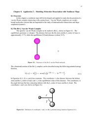
e.) Without solving any equations, sketch the expected form of the ground state
wavefunction for the system given above for E < V 0 . Qualitatively compare and
contrast this wavefunction with the ground state wavefunction for the particle in a
half-infinite well of the same width. Pay particular attention to the shape of the
wavefunctions in the various regions. €
Example graphs are shown below for the ground state wavefunctions for the system given in this problem
(with a finite width barrier) and the particle in a half-infinite well. These wavefunctions were constructed
using a box width of L=3 bohr for both systems, and a barrier width of 1.5 bohr for the finite barrier (i.e.,
L=3 and Q=4.5 bohr). In both cases the barrier height V 0 is 4.5 hartrees.
ψ(x)
0.006
0.005
0.004
0.003
0.002
Ground State (n=1)
This Problem €
Half-Infinite Well
ψ1(x)
0.9
0.8
0.7
0.6
0.5
0.4
0.3
0.001
0.000
0.0 2.0 4.0 6.0 8.0 10.0
-0.001
x (bohr)
0.2
0.1
0.0
0.0 2.0 4.0 6.0 8.0 10.0
-0.1
x (bohr)
In general, the shapes of the wavefunctions for the two systems are similar (note that the wavefunctions are
not normalized, so the scale on the y-axis for each is arbitrary). Since the wavefunctions correspond to
ground states, there are no nodes in the wavefunctions within the well or barrier regions. In addition, both
wavefunctions exhibit similar tunneling behavior in classically forbidden region III.
The differences between the two functions are most distinct in region IV. Here, the barrier in the halfinfinite
well continues to infinity, whereas in this problem the finite width of the barrier means that the
potential drops to 0 in region IV (for x>4.5 bohr in the example, or x>Q in general). The particle in the
half-infinite well has a wavefunction that continues to die off monotonically to 0 as x increases. On the
other hand, the particle trapped behind the finite barrier becomes free in region IV, and the wavefunction
therefore exhibits free particle-like behavior in this region. The oscillations of the free particle-like
wavefunction in region IV are low amplitude as a result of the small probability density for tunneling
through the barrier. However, the oscillations in the wavefunction continue undamped with wavelength
2π
k
for all x>Q.
€