Fuzzy c-means

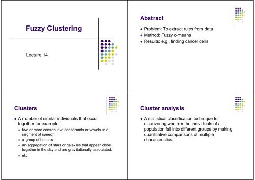
Abstract 

Fuzzy Clustering 

• Problem: To extract rules from data 

• Method: Fuzzy c-means 

• Results: e.g., finding cancer cells 

Lecture 14 

Clusters 

• A number of similar individuals that occur 

together for example: 

• two or more consecutive consonants or vowels in a 

segment of speech 

• a group of houses 

• an aggregation of stars or galaxies that appear close 

together in the sky and are gravitationally associated. 

• etc. 

Cluster analysis 

• A statistical classification technique for 

discovering whether the individuals of a 

population fall into different groups by making 

quantitative comparisons of multiple 

characteristics.

Vehicle Example 

Vehicle Clusters 

Vehicle Top speed 

km/h 

Colour Air 

resistance 

Weight 

Kg 

V1 220 red 0.30 1300 

V2 230 black 0.32 1400 

V3 260 red 0.29 1500 

V4 140 gray 0.35 800 

V5 155 blue 0.33 950 

V6 130 white 0.40 600 

V7 100 black 0.50 3000 

V8 105 red 0.60 2500 

V9 110 gray 0.55 3500 

Weight [kg] 

3500 

3000 

2500 

2000 

1500 

1000 

Lorries 

Medium market cars 

Sports cars 

500 

100 150 200 250 300 

Top speed [km/h] 

Terminology 

feature 

Weight [kg] 

3500 

3000 

2500 

2000 

1500 

1000 

Object or data point 

Lorries 

Medium market cars 

Sports cars 

500 

100 150 200 250 300 

Top speed [km/h] 

feature 

cluster 

label 

feature space 

Classify cracked tiles 

475Hz 557Hz Ok 

-----+-----+--- 

0.958 0.003 Yes 

1.043 0.001 Yes 

1.907 0.003 Yes 

0.780 0.002 Yes 

0.579 0.001 Yes 

0.003 0.105 No 

0.001 1.748 No 

0.014 1.839 No 

0.007 1.021 No 

0.004 0.214 No 

Table 1: frequency 

intensities for ten 

tiles. 

Tiles are made from clay moulded into the right shape, brushed, glazed, and baked. 

Unfortunately, the baking may produce invisible cracks. Operators can detect the 

cracks by hitting the tiles with a hammer, and in an automated system the response is 

recorded with a microphone, filtered, Fourier transformed, and normalised. A small set 

of data is given in TABLE 1 (adapted from MIT, 1997).

hard c-means (HCM) 

(also known as k means) 

2 

Tiles data: o = whole tiles, * = cracked tiles, x = centres 

2 


1 

1 

0 

0 

log(intensity) 557 Hz 

-1 

-2 

-3 

-4 

-5 


-1 

-2 

-3 

-4 

-5 

-6 

-6 

-7 

-7 

-8 

-8 -6 -4 -2 0 2 


Plot of tiles by frequencies (logarithms). The whole tiles (o) seem well separated 

from the cracked tiles (*). The objective is to find the two clusters. 

-8 

-8 -6 -4 -2 0 2 


1. Place two cluster centres (x) at random. 

2. Assign each data point (* and o) to the nearest cluster centre (x) 

2 


2 


1 

1 

0 

0 


-1 

-2 

-3 

-4 

-5 


-1 

-2 

-3 

-4 

-5 

-6 

-6 

-7 

-7 

-8 

-8 -6 -4 -2 0 2 


1. Compute the new centre of each class 

2. Move the crosses (x) 

-8 

-8 -6 -4 -2 0 2 


Iteration 2


2 

1 

0 

-1 

-2 

-3 

-4 

-5 

-6 

-7 


-8 

-8 -6 -4 -2 0 2 


Iteration 3 


2 

1 

0 

-1 

-2 

-3 

-4 

-5 

-6 

-7 


-8 

-8 -6 -4 -2 0 2 


Iteration 4 (then stop, because no visible change) 

Each data point belongs to the cluster defined by the nearest centre 

M = 

0.0000 1.0000 

0.0000 1.0000 

0.0000 1.0000 

0.0000 1.0000 

0.0000 1.0000 

1.0000 0.0000 

1.0000 0.0000 

1.0000 0.0000 

1.0000 0.0000 

1.0000 0.0000 

Membership matrix M 

m 

ik 

data point k cluster centre i 

⎧⎪ 

1 if u −c ≤ u −c 

= ⎨ 

⎪ ⎩0 

otherwise 

2 

k i k j 

distance 

2 

cluster centre j 

The membership matrix M: 

1. The last five data points (rows) belong to the first cluster (column) 

2. The first five data points (rows) belong to the second cluster (column)

c-partition 

Objective function 

All clusters C 

together fills the 

whole universe U 

Clusters do not 

overlap 

Minimise the total sum of 

all distances 

A cluster C is never 

empty and it is 

smaller than the 


c 

∪ 

i= 

1 

C = U 

C ∩ C = Ø 

i 

i 

Ø ⊂ C ⊂ U 

2 ≤ c ≤ K 

i 

j 

for all i ≠ j 

for all i 

There must be at least 2 

clusters in a c-partition and 

at most as many as the 

number of data points K 

J = 

c 

∑ 

J 

= 

c 

⎛ 

⎜ 

⎝ 

∑⎜ 

∑ 

i 

k 

i= 

1 i= 1 k , uk∈Ci 

u − c 

i 

2 

⎞ 

⎟ 

⎠ 

Fuzzy c-means 

One of the problems of the k-means algorithm is that it 

gives a hard partitioning of the data, that is to say that 

each point is attributed to one and only one cluster. 

But points on the edge of the cluster, or near another 

cluster, may not be as much in the cluster as points in 

the center of cluster. 


Therefore, in fuzzy clustering, each point does not pertain 

to a given cluster, but has a degree of belonging to a 

certain cluster, as in fuzzy logic. For each point x we have a 

coefficient giving the degree of being in the k-th cluster 

u k (x). Usually, the sum of those coefficients has to be one, 

so that u k (x) denotes a probability of belonging to a certain 

cluster:



The degree of being in a certain cluster is related to the 

inverse of the distance to the cluster 

With fuzzy c-means, the centroid of a cluster is computed as 

being the mean of all points, weighted by their degree of 

belonging to the cluster, that is: 

then the coefficients are normalized and fuzzyfied with a 

real parameter m > 1 so that their sum is 1. So : 


For m equal to 2, this is equivalent to normalising the 

coefficient linearly to make their sum 1. When m is close to 

1, then cluster center closest to the point is given much 

more weight than the others, and the algorithm is similar to 

k-means. 


The fuzzy c-means algorithm is greatly similar to the k- 

means algorithm :


•Choose a number of clusters 

•Assign randomly to each point coefficients for being in the 

clusters 

•Repeat until the algorithm has converged (that is, the 

coefficients' change between two iterations is no more than ε, 

the given sensitivity threshold) : 

•Compute the centroid for each cluster, using the formula 

above 

•For each point, compute its coefficients of being in the 

clusters, using the formula above 

Fuzzy C-means 

uij is membership of sample i to custer j 

ck is centroid of custer i 

while changes in cluster Ck 

% compute new memberships 

for k=1,…,K do 

for i=1,…,N do 

ujk = f(xj – ck) 

end 

end 

% compute new cluster centroids 

for k=1,…,K do 

% weighted mean 

ck = SUMj jkxk xj /SUMj ujk 

end 

end 


Fuzzy c-means (FCM) 

The fuzzy c-means algorithm minimizes intra-cluster 

variance as well, but has the same problems as k-means, 

the minimum is local minimum, and the results depend on 

the initial choice of weights. 


2 

1 

0 

-1 

-2 

-3 

-4 

-5 

-6 

-7 


-8 

-8 -6 -4 -2 0 2 


Each data point belongs to two clusters to different degrees

2 


2 


1 

1 

0 

0 


-1 

-2 

-3 

-4 

-5 


-1 

-2 

-3 

-4 

-5 

-6 

-6 

-7 

-7 

-8 

-8 -6 -4 -2 0 2 


-8 

-8 -6 -4 -2 0 2 


1. Place two cluster centres 

2. Assign a fuzzy membership to each data point depending on 

distance 

1. Compute the new centre of each class 

2. Move the crosses (x) 

2 


2 


1 

1 

0 

0 


-1 

-2 

-3 

-4 

-5 


-1 

-2 

-3 

-4 

-5 

-6 

-6 

-7 

-7 

-8 

-8 -6 -4 -2 0 2 


-8 

-8 -6 -4 -2 0 2 


Iteration 2 

Iteration 5

2 


2 


1 

1 

0 

0 


-1 

-2 

-3 

-4 

-5 


-1 

-2 

-3 

-4 

-5 

-6 

-6 

-7 

-7 

-8 

-8 -6 -4 -2 0 2 


-8 

-8 -6 -4 -2 0 2 


Iteration 10 

Iteration 13 (then stop, because no visible change) 

Each data point belongs to the two clusters to a degree 

M = 

0.0025 0.9975 

0.0091 0.9909 

0.0129 0.9871 

0.0001 0.9999 

0.0107 0.9893 

0.9393 0.0607 

0.9638 0.0362 

0.9574 0.0426 

0.9906 0.0094 

0.9807 0.0193 

Fuzzy membership matrix M 

Point k’s membership 

of cluster i 

m 

ik 

dik 

= 

c 

∑ 

j= 

1 

k 

1 

⎛ ⎞ 

⎜ 

dik 

⎟ 

⎝ d 

jk ⎠ 

= u − c 

i 

2 / 

( q−1) 

Fuzziness 

exponent 

Distance from point k to 

current cluster centre i 

Distance from point k to 

other cluster centres j 

The membership matrix M: 

1. The last five data points (rows) belong mostly to the first cluster (column) 

2. The first five data points (rows) belong mostly to the second cluster (column)

Fuzzy membership matrix M 

m ik = 

2 / ( q−1 

⎛ ⎞ 

) 

c 

dik 

= 

∑ 

j= 

1 

= 

⎛ d 

⎜ 

⎝ d 

d 

⎜ 

⎝ d 

ik 

1k 

1 

1 

jk 

2 /( q−1) 2 /( q−1) 2 /( q−1) 

⎞ 

⎟ 

⎠ 

⎟ 

⎠ 

⎛ d ⎞ ⎛ 

ik 

d 

+ ⎜ ⎟ + + 

⎜ 

⎝ d2k 

⎠ ⎝ d 

1 

2 /( q−1) 

dik 

1 

1 

+ + + 

2 /( q−1) 2 /( q−1) 2 /( q−1) 

1k 

d2k 

dck 

1 

ik 

ck 

⎞ 

⎟ 

⎠ 

Gravitation to 

cluster i relative 

to total gravitation 

Fuzzy Membership 

Membership of test point 

1 

0.5 

o is with q = 1.1, * is with q = 2 

0 

1 2 3 4 5 

Data point 

Cluster centres 

Fuzzy c-partition 

Example: Classify cancer cells 

All clusters C together fill the 

whole universe U. 

Remark: The sum of 

memberships for a data point 

is 1, and the total for all 

points is K 

A cluster C is never 

empty and it is 

smaller than the 


c 

∪ 

i= 

1 

C = U 

C ∩ C = Ø 

i 

i 

Ø ⊂ C ⊂ U 

2 ≤ c ≤ K 

i 

j 

for all i ≠ j 

for all i 

Not valid: Clusters 

do overlap 

There must be at least 2 

clusters in a c-partition and 

at most as many as the 

number of data points K 

Normal smear 

Using a small brush, cotton stick, or wooden 

stick, a specimen is taken from the uterin cervix 

and smeared onto a thin, rectangular glass plate, 

a slide. The purpose of the smear screening is to 

diagnose pre-malignant cell changes before they 

progress to cancer. The smear is stained using 

the Papanicolau method, hence the name Pap 

smear. Different characteristics have different 

colours, easy to distinguish in a microscope. A 

cyto-technician performs the screening in a 

microscope. It is time consuming and prone to 

error, as each slide may contain up to 300.000 

cells. 

Severely dysplastic smear 

Dysplastic cells have undergone precancerous changes. 

They generally have longer and darker nuclei, and they 

have a tendency to cling together in large clusters. Mildly 

dysplastic cels have enlarged and bright nuclei. 

Moderately dysplastic cells have larger and darker 

nuclei. Severely dysplastic cells have large, dark, and 

often oddly shaped nuclei. The cytoplasm is dark, and it 

is relatively small.

Possible Features 

Classes are nonseparable 

• Nucleus and cytoplasm area 

• Nucleus and cyto brightness 

• Nucleus shortest and longest diameter 

• Cyto shortest and longest diameter 

• Nucleus and cyto perimeter 

• Nucleus and cyto no of maxima 

• (...) 

Hard Classifier (HCM) 

Fuzzy Classifier (FCM) 

moderate 

moderate 

Ok 

light 

Ok 

severe 

A cell is either one 

or the other class 

defined by a colour. 

Ok 

light 

Ok 

severe 

A cell can belong to 

several classes to a 

Degree, i.e., one column 

may have several colours.

Function approximation 

Approximation by fuzzy sets 

Output1 

1.5 

1 

0.5 

0 

-0.5 

2 

1 

0 

-1 

-2 

0 0.1 0.2 0.3 0.4 0.5 0.6 0.7 0.8 0.9 1 

-1 

-1.5 

0 0.1 0.2 0.3 0.4 0.5 0.6 0.7 0.8 0.9 1 

Input 

Curve fitting in a multi-dimensional space is also called function 

approximation. Learning is equivalent to finding a function that best 

fits the training data. 

1 

0.8 

0.6 

0.4 

0.2 

0 

0 0.1 0.2 0.3 0.4 0.5 0.6 0.7 0.8 0.9 1 

Procedure to find a model 

1. Acquire data 

2. Select structure 

3. Find clusters, generate model 

4. Validate model 

Conclusions 

• Compared to neural networks, fuzzy models can 

be interpreted by human beings 

• Applications: system identification, adaptive 

systems

Fuzzy c-means

You also want an ePaper? Increase the reach of your titles

Delete template?

Save as template?