Homework 1: State Space Realization - Kckong.info
Homework 1: State Space Realization - Kckong.info
Homework 1: State Space Realization - Kckong.info

Create successful ePaper yourself
Turn your PDF publications into a flip-book with our unique Google optimized e-Paper software.
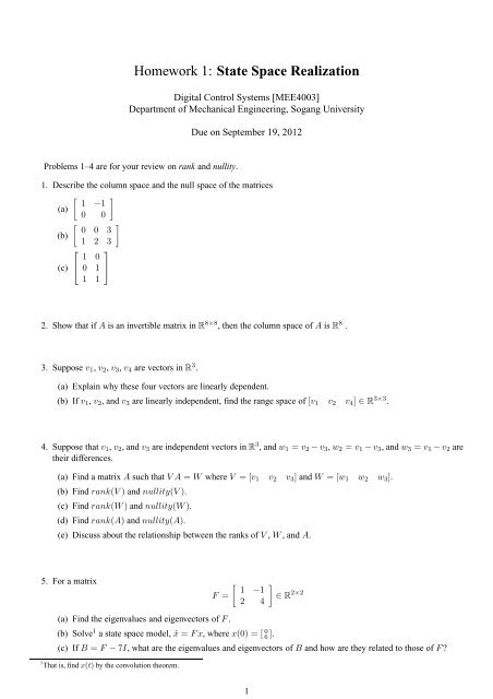
<strong>Homework</strong> 1: <strong>State</strong> <strong>Space</strong> <strong>Realization</strong><br />
Digital Control Systems [MEE4003]<br />
Department of Mechanical Engineering, Sogang University<br />
Due on September 19, 2012<br />
Problems 1–4 are for your review on rank and nullity.<br />
1. Describe the column space and the null space of the matrices<br />
[ ] 1 −1<br />
(a)<br />
0 0<br />
[ ] 0 0 3<br />
(b)<br />
1 2 3<br />
⎡ ⎤<br />
1 0<br />
(c) ⎣ 0 1 ⎦<br />
1 1<br />
2. Show that if A is an invertible matrix in R 8×8 , then the column space ofAisR 8 .<br />
3. Suppose v 1 ,v 2 ,v 3 ,v 4 are vectors inR 3 .<br />
(a) Explain why these four vectors are linearly dependent.<br />
(b) If v 1 , v 2 , and v 3 are linearly independent, find the range space of[v 1 v 2 v 4 ] ∈ R 3×3 .<br />
4. Suppose that v 1 ,v 2 , andv 3 are independent vectors inR 3 , andw 1 = v 2 −v 3 ,w 2 = v 1 −v 3 , andw 3 = v 1 −v 2 are<br />
their differences.<br />
(a) Find a matrix A such that VA = W where V = [v 1 v 2 v 3 ] and W = [w 1 w 2 w 3 ].<br />
(b) Find rank(V) and nullity(V).<br />
(c) Find rank(W) and nullity(W).<br />
(d) Find rank(A) and nullity(A).<br />
(e) Discuss about the relationship between the ranks of V , W , and A.<br />
5. For a matrix<br />
F =<br />
[ 1 −1<br />
2 4<br />
]<br />
∈ R 2×2<br />
(a) Find the eigenvalues and eigenvectors of F .<br />
(b) Solve 1 a state space model, ẋ = Fx, wherex(0) = [ 0 6 ].<br />
(c) If B = F −7I, what are the eigenvalues and eigenvectors ofB and how are they related to those of F <br />
1 That is, findx(t) by the convolution theorem.<br />
1
6. Calculate e Ft and F k , where k is an integer, for the matrices:<br />
[ ] 0 0<br />
(a) F =<br />
1 0<br />
[ ] 4 3<br />
(b) F =<br />
1 2<br />
[ ]<br />
0 1<br />
(c) F =<br />
−3 −2<br />
7. Consider a matrix<br />
⎡<br />
F =<br />
⎢<br />
⎣<br />
0 1 0 0 0<br />
0 0 1 0 0<br />
0 0 0 1 0<br />
0 0 0 0 1<br />
−45 −111 −104 −48 −11<br />
⎤<br />
⎥<br />
⎦<br />
(a) Using the Matlab function eig.m, show that the eigenvalues of F are−1, −2±j, −3, and −3.<br />
(b) Find V ∈ R 5×5 such that 2<br />
where<br />
⎡<br />
A =<br />
⎢<br />
⎣<br />
F = VAV −1<br />
−1 0 0 0 0<br />
0 −2 1 0 0<br />
0 −1 −2 0 0<br />
0 0 0 3 1<br />
0 0 0 0 3<br />
(c) Noting that the matrix A consists of three block matrices, solve e Ft .<br />
(d) For a state space equation, ẋ = Fx, findx(1) for x(0) = [ 1 1 1 1 1 ] T .<br />
⎤<br />
⎥<br />
⎦<br />
8. Suppose a state space model is given byẋ = Fx, where F ∈ R 2×2 . Suppose it is known that<br />
[ ] [ ] [ ] [<br />
4 1 5 1<br />
x(1) = for x(0) = and x(1) = for x(0) =<br />
−2 1<br />
−2 2<br />
]<br />
(a) Find e Ft .<br />
(b) Find x(10) for x(0) = [ 1 0 ].<br />
9. Consider a quarter vehicle model shown in Fig. 1a, where u is the force (input) applied to the vehicle.<br />
(a) Find the equation of motion of the simplified model shown in the figure.<br />
(b) Defining x 1 as the output of the system, find a state space model corresponding to the equation of motion. 3<br />
In other words, find the matrices F ,G, and H with appropriate dimensions:<br />
ẋ = Fx+Gu<br />
y = Hx<br />
(c) Assuming M 1 = 1000, M 2 = 100, k 1 = 20000, k 2 = 15000, c 1 = 10000, and c 2 = 40000, find the<br />
eigenvalues and eigenvectors of the state matrix F by the Matlab function, eig.m.<br />
2 Since V ∈ R 5×5 , all the elements of V should be real.<br />
3 Hint: you may define the statexas [ x 1 x 2 ẋ 1 ẋ 2<br />
] T<br />
∈ R 4 .<br />
2
0.09<br />
0.08<br />
The ¼ mass of a car M 1<br />
The mass of<br />
a tire M 2<br />
u<br />
c , k 1 1<br />
c1<br />
u<br />
M 1<br />
k 1<br />
x 1<br />
Position of M 1<br />
0.07<br />
0.06<br />
0.05<br />
0.04<br />
0.03<br />
0.02<br />
M 2<br />
x 2<br />
0.01<br />
c 2<br />
, k 2<br />
c 2<br />
k 2<br />
0<br />
0 5 10 15 20<br />
Time(sec)<br />
(a) A quarter vehicle model.<br />
(b) A simulation result.<br />
Figure 1: Settings for Problem 5.<br />
(d) Find V and Λ such that F = VΛV −1 and Λ is a diagonal matrix with the eigenvalues of F .<br />
(e) Calculate the position of M 1 (i.e., x 1 (t)), right after a driver of 70kg (approximately 700N) gets on the<br />
vehicle. That is,<br />
{<br />
700 for t ≥ 0<br />
u(t) =<br />
0 for t < 0<br />
You may use the Matlab function, lsim.m.<br />
(f) The driver left the vehicle at t = 10, i.e.<br />
⎧<br />
⎪⎨ 0 for t < 0<br />
u(t) = 700 for 0 ≤ t < 10<br />
⎪⎩<br />
0 for 10 ≤ t<br />
Calculate the position ofM 1 using lsim.m and plot y(t) versus t. 4 The graph should look like Fig. 1b.<br />
10. Given the system<br />
ẋ =<br />
[ −4 1<br />
−2 −1<br />
] [ 0<br />
x+<br />
1<br />
with zero initial conditions, find the steady-state value 5 of x for a unit step input u.<br />
]<br />
u<br />
4 Hint: you may define<br />
t = [0:0.001:20]; and<br />
u = zeros(1,20001); u(1:10000)=700*ones(1,10000);<br />
5 Hint: notice thatẋis zero at the steady state.<br />
3
![Digital Control Systems [MEE 4003] - Kckong.info](https://img.yumpu.com/40221932/1/184x260/digital-control-systems-mee-4003-kckonginfo.jpg?quality=85)
![Digital Control Systems [MEE 4003] - Kckong.info](https://img.yumpu.com/32606446/1/184x260/digital-control-systems-mee-4003-kckonginfo.jpg?quality=85)