paper (pdf) - Mathematics Archives

AN INTERESTING PROBLEM FROM CALCULUS
AND MUCH MORE
Robert Kreczner
University of Wisconsin Stevens Point
Stevens Point WI54481
Email: rkreczne@uwspmail.uwsp.edu
1. INTRODUCTION. In the latest Calculus; by J. Stewart, we can notice many new
problems which can be solved by using modern mathematical technologies, for example,
Mathematica and Geometer's Sketchpad. Solving these problems with the help of these
programs is not only more enjoyable, but in some cases may lead to profound
generalizations and discoveries.
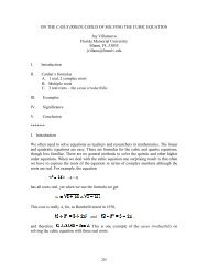
In this paper we will concentrate on one of such problems, the problem #78, on page 70.
This problem is stated there as follows: The figure shows a fixed circle C 1 with equation
2 2
(x 1) € y œ
1 and a shrinking circle C 2 with radius r and center the origin.
P is the point (0, r), Q is the upper point of intersection of the two circles, and R is the
point of intersection of the line PQ and the x-axis. What happens to R as C 2 shrinks,
that is, as r p 0 €
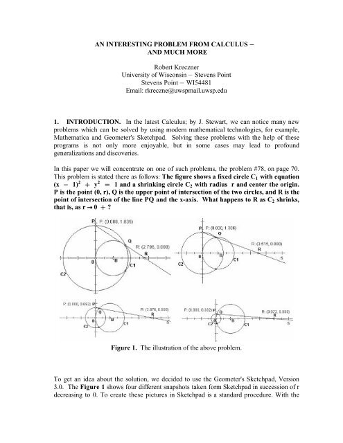
Figure 1. The illustration of the above problem.
To get an idea about the solution, we decided to use the Geometer's Sketchpad, Version
3.0. The Figure 1 shows four different snapshots taken form Sketchpad in succession of r
decreasing to 0. To create these pictures in Sketchpad is a standard procedure. With the

Sketchpad, we can keep shrinking continuously the circle C 2 by dragging with mouse the
point P towards origin, and at the same time observing that the point R approaches the
number 4. Furthermore, by taking advantage that the drawings in the Sketchpad are
dynamic, we can easily change the circle C 1 to a circle of any radius r, and make an
observation that the point R approaches the number 4 † r.
A similar exercise can be carry out for the problem in which the circle C 1 is
replaced be a straight line with positive slope passing through origin. This time we will
observe that the point R approaches 0.
2. GENERALIZATION. The described above problem can be easily generalized by
replacing the fixed circle C1 by any curve. In the Figure 2 below, this curve is denoted
again by C 1 . Since we are going to shrink the circle C 2 , the only important part of the
curve is the part that is immediately close to origin. Therefore, naturally we can assume
that the curve C 1 passes through the origin, is smooth enough; and for positive x close to
origin, it lies in the first quadrant, and is increasing there.
Figure 2.
Thus our problem, with these assumptions, is to find limit of the point R as radius r of
circle C approaches 0
2 .
3. SETTING UP FOR GENERAL SOLUTION. In this paragraph, We will refer to the
notation of the Figure 2. If the curve C 1 is given by an equation F(x, y) œ 0, then the
coordinates of the point Q œ (x, y), the point of intersection of the circle C 2 and the
curve C 1, can be found by solving system of equations,
2 2 2
F(x, y) œ 0 and x € y œ r (3.1)

Then, the equation of the line through the points P and Q is
Y r X . (3.2)
x
Setting Y œ 0 in the equation (3.2), we get the x-coordinate of the point R,
Thus, our problem is to find
œ Y r
rx
y r
X œ . (3.3)
rx
lim , (3.4)
y r
rp0+
which we denote by limtR.
However, this problem as simple as it might seem at the first sight, to carry out this
computation, even for simple equations F(x, y) œ 0, is very laborious and tedious, or
even impossible to do especially for most students. There are three main reasons for these,
the system of equations (3.1) is to difficult or impossible to solve, the expression (3.3) is
lengthy, and thus the computation of limit (3.4) is not clear. In contrast, with the
Mathematica all these difficulties might be avoided, especially if the equation F(x,y) œ 0 is
relatively simple. In this paper we decided restrict ourselves to the cases when the equation
F(x,y) œ 0 represents conics. We also must remember that our goal is not to do the
computations, but make a discovery.
4. MATHEMATICA IN ACTION. We will apply the Mathematica to do all the
computations described in the paragraph 3. To do these we can use the following program.
# # #
pointQ:=Solve[{x € y œ =r , F(x,y) œ
=0}, {(x, y}]
pointR:=(r*x)/(r
y)/. {pointQ[[4]][[1]], pointQ[[4]][2]]}
limitR= Limit[ pointR, r >0}
Warning: For some reason, if the equation F(x,y) œ 0 have a parameter, the Limit
command produces incorrect output. For example, for parabola given by equation y
# œ 2 a
x, the output is 0, which is incorrect. However, if we define the parameter a to be the
number E or Pi, the Limit is computed correctly, and at the same time we can see the
answer in general form since E and Pi being transcendental numbers will not cancel out
during symbolic computation. Thus, in the above program we can line a: œ Pi, and so on.
The intermediate results of this computation we will illustrate for parabola
y # œ 2ax only, the final results for the other curves are included in Table 1, the middle
column.

In[1]:=
PointQ=Solve[{x^2 € y^2==r^2, y^2==2 a x},{x,y}]
Out[1]=
# % # #
2 a 2 Sqrt[a € a r ]
# % # #
2 a
{{x > , y > Sqrt[ 2 a 2 Sqrt[a € a r ]},
# % # #
2 a 2 Sqrt[a € a r ]
# % # #
2 a
{x > , y > Sqrt[ 2 a 2 Sqrt[a € a r ]},
# % # #
2 a € 2 Sqrt[a € a r ]
# % # #
2 a
{x > , y > Sqrt[ 2 a € 2 Sqrt[a € a r ]},
# % # #
2 a +2 Sqrt[a € a r ]
# % # #
2 a
{x > , y > Sqrt[ 2 a € 2 Sqrt[a € a r ]}}
In[2]:=
pointR=(r x)/(r
y)/ { pointQ[[4]][[1]], pointQ[[4]][[2]]}
†
Out[3]=
# % # #
r( 2 a € 2 Sqrt[a € a r ])
2a (r Sqrt[ 2 a# € 2 Sqrt[a% € a
#
r
#]])
In[4]:=
a:=Pi
In[5]:=
limitR=Limit[pointR, r >0]
Out[5]=
4 Pi
5. LITTLE DISCUSSION. Before we show the results of our computation, we would
like to discuss the possible solutions. Our first guess is that limit of R depends on the
tangent line to the curve C 1 at origin. However, this assertion has to be rejected since for
any line passing through the origin the point R tends to the origin. The second guess is that
this limit should depend on the curvature of curve C 1 at origin, since the curvature fully

characterizes a curve. Keeping these remarks in our mind, the analysis of the Table 1
should bring the desired discovery
Figure 3. Illustration of the main Theorem.
Curve Limit of R Curvature at Origin
Line y œ ax 0 0
Circle (x
2 2
r) € y œ
2
r 4r
1
r
(x
2
a)
2
y
2
4b a
a2 b2 a b
2
2
(x € a)
2
y
2
4b a
a
2
b
2
a b
2
2 2 2 2 1
a € b
Ellipse € œ 1
Hyperbola œ 1
Circle (x a) € (y b) œ a € b 0
È
Table 1.
6. MAIN DISCOVERY. Under the assumptions of Paragraph 2, observations made out
of the Table 1, and notations of Figure 3, we can state the following
THEOREM. If the curvature circle C 3 of a curve C 1 at origin has radius 3and its center
lies on x-axis, then the point R approaches number 4 3. Otherwise, the point R approaches
origin.
Proof. We will give only the proof for the case when the center of curvature lies on x-
axis, this is illustrated by Figure 3. For the other case the proof is the same.
Let % ž 0 be any real number, and C 4 be the circle with radius 3 € % and center
( 3 € %, 0). The points S and T are the x-intercepts of the lines passing through the point P
and the intersection points of the circle C 2 with the circles C 3 and C 4, respectively. Then,
since we assumed that the curve C1is concave down in the first quadrant, close to origin,
we observe that the point R is between the points S and T. From the Table 1, we know that
S and T tend to 43 and 4( 3 € %) respectively, as r >0 . Therefore, limit of R is also
between 43and 4( 3 € %). Since % is any real positive number, limit of R must be 43.
2 2

REFERENCES
1. James Stewart, Calculus; Early Transcendentals, 3rd edition, Brooks/Cole, 1994.