using excel solver in optimization problems - Mathematics Archives

USING EXCEL SOLVER IN OPTIMIZATION PROBLEMS
Leslie Chandrakantha
John Jay College of Criminal Justice of CUNY
Mathematics and Computer Science Department
445 West 59 th Street, New York, NY 10019
lchandra@jjay.cuny.edu
Abstract
We illustrate the use of spreadsheet modeling and Excel Solver in solving linear and
nonlinear programming problems in an introductory Operations Research course. This is
especially useful for interdisciplinary courses involving optimization problems. We work
through examples from different areas such as manufacturing, transportation, financial
planning, and scheduling to demonstrate the use of Solver.
Introduction
Optimization problems are real world problems we encounter in many areas such as
mathematics, engineering, science, business and economics. In these problems, we find
the optimal, or most efficient, way of using limited resources to achieve the objective of
the situation. This may be maximizing the profit, minimizing the cost, minimizing the
total distance travelled or minimizing the total time to complete a project. For the given
problem, we formulate a mathematical description called a mathematical model to
represent the situation. The model consists of following components:
• Decision variables: The decisions of the problem are represented using symbols
such as X 1 , X 2 , X 3 ,…..X n . These variables represent unknown quantities (number
of items to produce, amounts of money to invest in and so on).
• Objective function: The objective of the problem is expressed as a mathematical
expression in decision variables. The objective may be maximizing the profit,
minimizing the cost, distance, time, etc.,
• Constraints: The limitations or requirements of the problem are expressed as
inequalities or equations in decision variables.
If the model consists of a linear objective function and linear constraints in decision
variables, it is called a linear programming model. A nonlinear programming model
consists of a nonlinear objective function and nonlinear constraints. Linear programming
is a technique used to solve models with linear objective function and linear constraints.
The Simplex Algorithm developed by Dantzig (1963) is used to solve linear programming
problems. This technique can be used to solve problems in two or higher dimensions.
42

In this paper we show how to use spreadsheet modeling and Excel Solver for solving
linear and nonlinear programming problems.
Spreadsheet Modeling and Excel Solver
A mathematical model implemented in a spreadsheet is called a spreadsheet model.
Major spreadsheet packages come with a built-in optimization tool called Solver. Now
we demonstrate how to use Excel spreadsheet modeling and Solver to find the optimal
solution of optimization problems.
If the model has two variables, the graphical method can be used to solve the model.
Very few real world problems involve only two variables. For problems with more than
two variables, we need to use complex techniques and tedious calculations to find the
optimal solution. The spreadsheet and solver approach makes solving optimization
problems a fairly simple task and it is more useful for students who do not have strong
mathematics background.
The first step is to organize the spreadsheet to represent the model. We use separate
cells to represent decision variables, create a formula in a cell to represent the objective
function and create a formula in a cell for each constraint left hand side. Once the
model is implemented in a spreadsheet, next step is to use the Solver to find the
solution. In the Solver, we need to identify the locations (cells) of objective function,
decision variables, nature of the objective function (maximize/minimize) and
constraints.
Example One (Linear model): Investment Problem
Our first example illustrates how to allocate money to different bonds to maximize the
total return (Ragsdale 2011, p. 121).
A trust office at the Blacksburg National Bank needs to determine how to invest
$100,000 in following collection of bonds to maximize the annual return.
Bond
Annual Maturity Risk Tax-Free
Return
A 9.5% Long High Yes
B 8.0% Short Low Yes
C 9.0% Long Low No
D 9.0% Long High Yes
E 9.0% Short High No
The officer wants to invest at least 50% of the money in short term issues and no more
than 50% in high-risk issues. At least 30% of the funds should go in tax-free investments,
and at least 40% of the total return should be tax free.
Creating the Linear Programming model to represent the problem:
Decision variables are the amounts of money should be invested in each bond.
X 1 = Amount of money to invest in Bond A
43

X 2 = Amount of money to invest in Bond B
X 3 = Amount of money to invest in Bond C
X 4 = Amount of money to invest in Bond D
X 5 = Amount of money to invest in Bond E
Objective Function:
Objective is to maximize the total annual return.
Maximize f(X 1 , X 2 , X 3 , X 4 , X 5 ) = 9.5%X 1 + 8%X 2 + 9%X 3 + 9%X 4 + 9%X 5
Constraints:
Total investment:
X 1 + X 2 + X 3 + X 4 + X 5 = 100,000.
At least 50% of the money goes to short term issues:
X 2 + X 5 >= 50,000.
No more than 50% of the money should go to high risk issues:
X 1 + X 4 + X 5 = 30,000.
At least 40% of the total annual return should be tax free:
9.5%X 1 + 8%X 2 + 9%X 4 >= 40%(9.5%X 1 + 8%X 2 + 9%X 3 + 9%X 4 + 9%X 5 )
Nonnegativity constraints (all the variables should be nonnegative):
X 1 , X 2 , X 3 , X 4 , X 5 >= 0.
Complete linear programming model:
Max: .095X 1 + .08X 2 + .09X 3 +.09X 4 + .09X 5
Subject to:
X 1 + X 2 + X 3 + X 4 + X 5 = 100,000.
X 2 + X 5 >= 50,000.
X 1 + X 4 + X 5 = 30,000.
9.5%X 1 + 8%X 2 + 9%X 4 >= 40%(9.5%X 1 + 8%X 2 + 9%X 3 + 9%X 4 + 9%X 5 )
X 1 , X 2 , X 3 , X 4 , X 5 >= 0.
Spreadsheet model and Solver implementation:
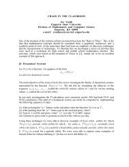
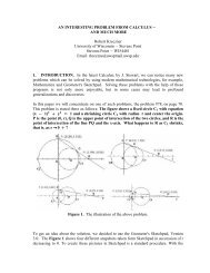
Implementing the problem in an Excel spreadsheet and Solver formulation produces the
following spreadsheet and Solver parameters. The cells B6 through B10 represent the
five decision variables. The cell C13 represents the objective function. The cells B11,
E11, G11, I11, B14, and B15 represent the constraint left hand sides. The nonnegativity
constraint is not implemented in the spreadsheet and it can be implemented in the
Solver. The complete set of constraints, target cell (objective function cell), variable cells
(changing cells) and whether to maximize or minimize the objective function are
identified in the Solver parameters box.
44

Figure 1: Spreadsheet implementation of example one
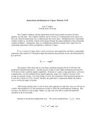
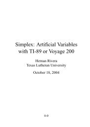
Figure 2: Solver implementation of example one
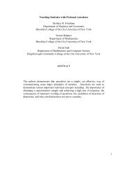
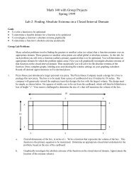
Figure 3: Spreadsheet with optimal solution of example one
45

Optimal money allocation:
Amount invested in Bond A = X 1 = $20, 339.
Amount invested in Bond B = X 2 = $20, 339.
Amount invested in Bond C = X 3 = $29, 661.
Amount invested in Bond D = X 4 = $0.
Amount invested in Bond E = X 5 = $29, 661.
The Maximum annual return is $8,898.00
Example Two (Nonlinear model): Network Flow Problem
This example illustrates how to find the optimal path to transport hazardous material (
Ragsdale, 2011, p.367)
Safety Trans is a trucking company that specializes transporting extremely valuable and
extremely hazardous materials. Due to the nature of the business, the company places
great importance on maintaining a clean driving safety record. This not only helps keep
their reputation up but also helps keep their insurance premium down. The company is
also conscious of the fact that when carrying hazardous materials, the environmental
consequences of even a minor accident could be disastrous.
Safety Trans likes to ensure that it selects routes that are least likely to result in an
accident. The company is currently trying to identify the safest routes for carrying a load
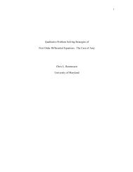
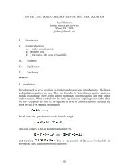
of hazardous materials from Los Angeles to Amarillo, Texas. The following network
summarizes the routes under consideration. The numbers on each arc represent the
probability of having an accident on each potential leg of the journey.
Las Vegas
0.003
Los Angeles
1
3
2
0.004 0.002
0.006
0.010 0.006
4
6
5
7
Figure 4: Network diagram of example two
8
0.001
Amarillo
0.002
0.010 0.004
0.006
0.009
Phoenix
San Diego
0.010
Tucson
Flagstaff
0.001
Albuquerque
10
0.005
0.002
0.003
Las Cruces
9
0.003
Lubbock
46

The objective is to find the route that minimizes the probability of having an accident, or
equivalently, the route that maximizes the probability of not having an accident.
Creating the mathematical model to represent the problem:
Each decision variable indicates whether or not a particular route is taken (they are
known as binary variables). We will define these variables in following way:
X ij = 1 , if the route from node i to node j is selected, and X ij = 0 otherwise.
Let P ij be the probability of having an accident while travelling from node i to node j
(1- P ij is the probability of not having an accident).
Objective function:
Minimize the probability of having an accident or equivalently, maximize the probability
of not having an accident. Note that this objective function is nonlinear.
Maximize f(X 12 , X 13 ,….) = (1-P 12 *X 12 ) (1-P 13 *X 13 ) (1 – P 14 *X 14 ) (1 – P 24 *X 24 ) ………. (1 -
P 9.10 *X 9,10 )
Constraints:
We use the following strategy to construct constraints: That is, supply one unit at the
starting node and demand one unit at the ending node, and for every other node,
demand or supply is zero. We find the route in which the one unit travels.
Total supply = 1, and total demand = 1, so for each node,
Net flow (Inflow – Outflow) = demand or supply for that node (Balance of flow rule).
Then we have following set of constraints:
Node 1: - X 12 – X 13 – X 14 = -1
Node 2: + X 12 – X 24 – X 26 = 0
Node 3: + X 13 – X 34 – X 35 = 0
Node 4: + X 14 + X 24 + X 34 – X 45 – X 46 – X 48 = 0
Node 5: + X 35 + X 45 – X 57 = 0
Node 6: + X 26 + X 46 - X 67 – X 68 = 0
Node 7: + X 57 + X 67 – X 78 – X 7,10 = 0
Node 8: + X 48 + X 68 + X 78 – X 8,10 = 0
Node 9: + X 79 – X 9,10 = 0
Node 10: + X 7,10 + X 8,10 + X 9,10 = 1
Complete nonlinear Programming model:
Maximize: (1-P 12 *X 12 ) (1-P 13 *X 13 ) (1 – P 14 *X 14 ) (1 – P 24 *X 24 ) ………. (1-P 9.10 *X 9,10 )
Subject to:
- X 12 – X 13 – X 14 = -1
+ X 12 – X 24 – X 26 = 0
+ X 13 – X 34 – X 35 = 0
47

+ X 14 + X 24 + X 34 – X 45 – X 46 – X 48 = 0
+ X 35 + X 45 – X 57 = 0
+ X 26 + X 46 - X 67 – X 68 = 0
+ X 57 + X 67 – X 78 – X 7,10 = 0
+ X 48 + X 68 + X 78 – X 8,10 = 0
+ X 79 – X 9,10 = 0
+ X 7,10 + X 8,10 + X 9,10 = 1
All X ij are binary.
Spreadsheet model and Solver implementation:
Figure 5: Spreadsheet implementation of example Two
Figure 6: Solver implementation of example two
48

Figure 7: Spreadsheet with optimal solution of example two
The optimal path:
The route that minimizes the probability of having an accident is given below:
Los Angeles to Phoenix
Phoenix to Flagstaff
Flagstaff to Albuquerque
Albuquerque to Amarillo.
Conclusion:
Optimization problems in many fields can be modeled and solved using Excel Solver. It
does not require knowledge of complex mathematical concepts behind the solution
algorithms. This way is particularly helpful for students who are non math majors and
still want to take theses courses.
References:
1) Cliff T. Ragsdale, 2011, Spreadsheet Modeling and Decision Analysis, 6 th Edition.
SOUTH-WESTERN, Cengage Learning.
2) Dantzig, G. B. 1963, Linear Programming and Extensions, Princeton University
Press, Princeton, NJ.
3) John Walkenbach, 2007, Excel 2007 Formulas, John Wiley and Sons.
49