Problem Set 2 solutions - MIT Database Group
Problem Set 2 solutions - MIT Database Group
Problem Set 2 solutions - MIT Database Group

Create successful ePaper yourself
Turn your PDF publications into a flip-book with our unique Google optimized e-Paper software.
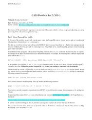
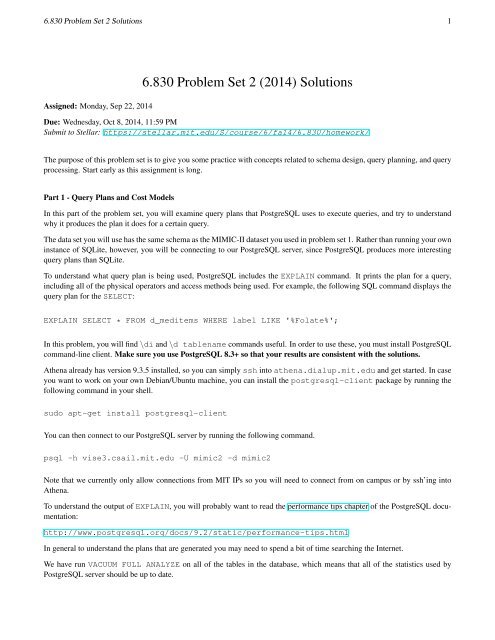
6.830 <strong>Problem</strong> <strong>Set</strong> 2 Solutions 1<br />
Assigned: Monday, Sep 22, 2014<br />
6.830 <strong>Problem</strong> <strong>Set</strong> 2 (2014) Solutions<br />
Due: Wednesday, Oct 8, 2014, 11:59 PM<br />
Submit to Stellar: https://stellar.mit.edu/S/course/6/fa14/6.830/homework/<br />
The purpose of this problem set is to give you some practice with concepts related to schema design, query planning, and query<br />
processing. Start early as this assignment is long.<br />
Part 1 - Query Plans and Cost Models<br />
In this part of the problem set, you will examine query plans that PostgreSQL uses to execute queries, and try to understand<br />
why it produces the plan it does for a certain query.<br />
The data set you will use has the same schema as the MIMIC-II dataset you used in problem set 1. Rather than running your own<br />
instance of SQLite, however, you will be connecting to our PostgreSQL server, since PostgreSQL produces more interesting<br />
query plans than SQLite.<br />
To understand what query plan is being used, PostgreSQL includes the EXPLAIN command. It prints the plan for a query,<br />
including all of the physical operators and access methods being used. For example, the following SQL command displays the<br />
query plan for the SELECT:<br />
EXPLAIN SELECT * FROM d_meditems WHERE label LIKE '%Folate%';<br />
In this problem, you will find \di and \d tablename commands useful. In order to use these, you must install PostgreSQL<br />
command-line client. Make sure you use PostgreSQL 8.3+ so that your results are consistent with the <strong>solutions</strong>.<br />
Athena already has version 9.3.5 installed, so you can simply ssh into athena.dialup.mit.edu and get started. In case<br />
you want to work on your own Debian/Ubuntu machine, you can install the postgresql-client package by running the<br />
following command in your shell.<br />
sudo apt-get install postgresql-client<br />
You can then connect to our PostgreSQL server by running the following command.<br />
psql -h vise3.csail.mit.edu -U mimic2 -d mimic2<br />
Note that we currently only allow connections from <strong>MIT</strong> IPs so you will need to connect from on campus or by ssh’ing into<br />
Athena.<br />
To understand the output of EXPLAIN, you will probably want to read the performance tips chapter of the PostgreSQL documentation:<br />
http://www.postgresql.org/docs/9.2/static/performance-tips.html<br />
In general to understand the plans that are generated you may need to spend a bit of time searching the Internet.<br />
We have run VACUUM FULL ANALYZE on all of the tables in the database, which means that all of the statistics used by<br />
PostgreSQL server should be up to date.
6.830 <strong>Problem</strong> <strong>Set</strong> 2 Solutions 2<br />
1. [15 points]: Query Plans<br />
Run the following query (using EXPLAIN) in PostgreSQL and answer questions (a) – (f) below:<br />
EXPLAIN SELECT ci.itemid, ci.label, count(*)<br />
FROM d_chartitems ci,<br />
chartevents ce,<br />
d_patients p,<br />
demographic_detail d<br />
WHERE ci.itemid = ce.itemid<br />
AND d.subject_id = p.subject_id<br />
AND ce.subject_id = p.subject_id<br />
AND d.overall_payor_group_descr = 'MEDICAID'<br />
AND p.sex = 'F'<br />
AND ce.icustay_id IS NOT NULL<br />
GROUP BY ci.itemid, ci.label<br />
ORDER BY ci.itemid, ci.label;<br />
a. What physical plan does PostgreSQL use Your answer should consist of a drawing of a query tree annotated with<br />
the access method types and join algorithms (note that you can use the pgadmin3 tool shown in class to draw plans,<br />
but will need to annotate them by hand.)<br />
b. Why do you think PostgreSQL selected this particular plan<br />
Choice of access methods:<br />
– Postgres does a sequential scan of demographic detail, d patients, and d chartitems because there<br />
are no indexes on those tables.<br />
– Postgres does an index scan on chartevents as part of an index nested loops join because it does not<br />
expect many tuples to be output from the previous join between demographic detail and d patients.<br />
Therefore, it expects that the small amount of random I/O required to seek for each record in the<br />
B-tree will cost less than the sequential I/O required to scan the entire table<br />
Choice of join algorithms:<br />
– Postgres performs a nested loops join between demographic detail and d patients because it expects<br />
so few rows from each table that it’s not worth the overhead to build an in-memory hash table.<br />
– See above for the reasoning behind the index nested loops join with chartevents
6.830 <strong>Problem</strong> <strong>Set</strong> 2 Solutions 3<br />
– Postgres performs a hash join with d chartitems because there are too many rows for a nested loops<br />
join to be practical.<br />
Join ordering:<br />
– Postgres chose this join ordering because it’s left-deep, it avoids any cross-products, and the first<br />
tables joined are most selective.<br />
c. What does PostgreSQL estimate the size of the result set to be<br />
Postgres estimates the size of the result set to be 4832 rows, with an average width of 17 bytes.<br />
d. When you actually run the query, how big is the result set<br />
It actually returns 674 rows.<br />
e. Run some queries to compute the sizes of the intermediate results in the query. Where do PostgreSQL’s estimates<br />
differ from the actual intermediate result cardinalities<br />
Postgres accurately predicts the number of rows for each sequential scan, but otherwise its estimates<br />
are incorrect:<br />
f. Given the tables and indices we have created, do you think PostgreSQL selected the best plan You can list all<br />
indices with \di, or list the indices for a particular table with \d tablename. If not, what would be a better<br />
plan Why<br />
Even though Postgres’ statistics were not always accurate, they were close enough (within an order of<br />
magnitude). The access methods, join ordering, and choice of join algorithms still make sense for the<br />
same reasons as described in part b.
6.830 <strong>Problem</strong> <strong>Set</strong> 2 Solutions 4<br />
2. [15 points]: Estimating Cost of Query Plans<br />
Use EXPLAIN to find the query plans for the following two queries and answer question (a).<br />
1. EXPLAIN SELECT m.label<br />
FROM d_chartitems AS c,<br />
chartevents AS ce,<br />
medevents AS me,<br />
d_meditems AS m<br />
WHERE c.itemid=ce.itemid<br />
AND ce.subject_id=me.subject_id<br />
AND me.itemid=m.itemid<br />
AND ce.subject_id > 100<br />
AND m.itemid>370;<br />
2. EXPLAIN SELECT m.label<br />
FROM d_chartitems AS c,<br />
chartevents AS ce,<br />
medevents AS me,<br />
d_meditems AS m<br />
WHERE c.itemid=ce.itemid<br />
AND ce.subject_id=me.subject_id<br />
AND me.itemid=m.itemid<br />
AND ce.subject_id > 27000<br />
AND m.itemid>370;<br />
a. Notice that the query plans for the two queries above are different, even though they have the same general form.<br />
Explain the difference in the query plan that PostgreSQL chooses, and explain why you think the plans are different.<br />
The first query has a much less selective filter condition on subject id than the second query. As a result,<br />
Postgres produces different plans for each query.<br />
Access methods: Since Postgres predicts it will scan many rows in the first query, it does not perform any index<br />
scans. The second query scans many fewer rows, however, so it makes sense to perform an index scan on<br />
chartevents and medevents.<br />
Join algorithms: The first query only uses hash joins and merge joins, since any other algorithm would be way<br />
too expensive. The second query uses an index nested loops join since it does not expect many tuples to be<br />
returned from the join between d chartitems and chartevents.<br />
Join order: The second query has a traditional left-deep plan with the most selective join first. The first query<br />
has a “bushy” plan, which Postgres determined through complex cost analysis to be the best plan.<br />
Now use EXPLAIN to find the query plan for the following query, and answer questions (b) – (g).<br />
3. EXPLAIN SELECT m.label<br />
FROM d_chartitems AS c,<br />
chartevents AS ce,<br />
medevents AS me,<br />
d_meditems AS m<br />
WHERE c.itemid=ce.itemid<br />
AND ce.subject_id=me.subject_id<br />
AND me.itemid=m.itemid<br />
AND ce.subject_id > 26300<br />
AND m.itemid>370;
6.830 <strong>Problem</strong> <strong>Set</strong> 2 Solutions 5<br />
b. What is PostgreSQL doing for this query How is it different from the previous two plans that are generated You<br />
may find it useful to draw out the plans (or use pgadmin3) to get a visual representation of the differences, though<br />
you are not required to submit drawings of the plans in your answer.<br />
This query is has a slightly less selective filter condition than query 2, but still much more selective than<br />
query 1. The only difference between this plan and the plan for query 1 is that there is an index scan<br />
on chartevents rather than a sequential scan. This is due to the fact that there are many fewer expected<br />
rows from chartevents after filtering.<br />
c. Run some more EXPLAIN commands using this query, sweeping the constant after the ’>’ sign from 100 to 27000.<br />
For what value of subject id does PostgreSQL switch plans<br />
Note: There might be additional plans other than these three. If you find this to be the case, please write the<br />
estimated last value of subject id for which PostgreSQL switches query plans.<br />
Switch 1: 14854 → 14855<br />
Switch 2: 26319 → 26320<br />
d. Why do you think it decides to switch plans at the values you found Please be as quantitative as possible in your<br />
explanation.<br />
Switch 1: According to EXPLAIN, Postgres expects 5971620 rows to be returned from scanning chartevents<br />
with ce.subject id > 14854. With ce.subject id > 14855, it expects 5930164 rows. Postgres likely estimates<br />
that the cost of random I/O for 5971620 seeks is higher than the cost to scan the entire table, while<br />
the cost of random I/O for 5930164 seeks is less than the cost to scan the entire table.<br />
Switch 2: When ce.subject id > 26319, Postgres expects 56224 rows to be returned from scanning<br />
chartevents. When ce.subject id > 26320, however, Postgres only expects 1 row to be returned from<br />
scanning chartevents. This drastic difference in expected rows explains the drastic difference between<br />
the plans.<br />
e. Suppose the crossover point (from the previous question) between queries 2 and 3 is subject id 23 . Compare the<br />
actual running times corresponding to the two alternative query plans at the crossover point. How much do they<br />
differ Do the same for all switch points.<br />
Inside psql, you can measure the query time by using the \timing command to turn timing on for all queries. To<br />
get accurate timing, you may also wish to redirect output to /dev/null, using the command \o /dev/null;<br />
later on you can stop redirection just by issuing the \o command without any file name. You may also wish to run<br />
each query several times, throwing out the first time (which may be longer if the data is not resident in the buffer<br />
pool) and averaging the remaining runs.<br />
Switch 1: Before the crossover point, the query takes about 65.3 ms. After, it takes about 64.9 ms.<br />
Switch 2: Before the crossover point, the query takes about 63.2 ms. After, it takes about 1.6 ms.<br />
f. Based on your answers to the previous two problems, are those switch points actually the best place to switch<br />
plans, or are they overestimate/underestimate of the best crossover points If they are not the actual crossover point,<br />
can you estimate the actual best crossover points without running queries against the database State assumptions<br />
underlying your answer, if any.<br />
Based on the runtimes calculated in part e, the first switch point seems like a good place to switch. Since<br />
the times are nearly equal, Postgres must have accurately calculated the tradeoff between random I/O<br />
in the index scan and sequential I/O in the sequential scan. Based on the answer to part d, the second<br />
switch point also seems like a good place to switch since the number of expected rows is so drastically<br />
different.
6.830 <strong>Problem</strong> <strong>Set</strong> 2 Solutions 6<br />
Part 2 – Query Plans and Access Methods<br />
In this problem, your goal is to estimate the cost of different query plans and think about the best physical query plan for a SQL<br />
expression.<br />
Suppose you are running a web service, “sickerthanyou.com”, where users can upload their genome data, and that uses genome<br />
processing algorithms to provide reports to users about their genetic disorders.<br />
Data is uploaded as files, with metadata about those files stored in a database table. Each file is passed through one or more<br />
fixed processing pipelines, which produce information about the disorders a patient has. These results are stored in another<br />
database table.<br />
The database contains the following tables:<br />
// user u_uid with a name, gender, age, and race<br />
CREATE TABLE users(u_uid int PRIMARY KEY,<br />
u_name char(50),<br />
u_gender char,<br />
u_age int,<br />
u_race int)<br />
// relatives table records familial relationships between users<br />
// relationships are not symmetric, so e.g., if A is B's child, then<br />
// there will be two entries: (A,B,child) and (B,A,parent)<br />
CREATE TABLE relatives(rl_uid1 int,<br />
rl_uid2 int,<br />
rel_type int,<br />
PRIMARY KEY (rl_uid1, rl_uid2));<br />
// data set collected about a specific user on a specific<br />
// genome sequencing platform,<br />
// with results stored in a specified file<br />
CREATE TABLE datasets(d_did int PRIMARY KEY,<br />
d_time timestamp,<br />
d_platform char(20),<br />
d_uid int REFERENCES users(u_uid),<br />
d_file char(100));<br />
// results produced by processing pipeline<br />
// each disorder column represents a specific condition<br />
// (e.g., disorder1 might be diabetes, disorder2 might be a type of cancer, etc.)<br />
CREATE TABLE results(r_rid int PRIMARY KEY,<br />
r_did int REFERENCES datasets(d_did),<br />
r_uid int REFERENCES users(u_uid),<br />
r_pipeline_version int,<br />
r_timestamp int,<br />
r_disorder1probability float,<br />
...<br />
r_disorder50probability float)<br />
In this database, int, timestamp, and float values are 8 bytes each and characters are 1 byte. All tuples have an additional<br />
8 byte header. This means, that, for example, the size of a single results record is 8 + 8 × 5 + 8 × 50 = 448 bytes.<br />
You create these tables in a row-oriented database. The system supports heap files and B+-trees (clustered and unclustered).<br />
B+-tree leaf pages point to records in the heap file. Assume that you can have at most one clustered index per file, and that
6.830 <strong>Problem</strong> <strong>Set</strong> 2 Solutions 7<br />
the database system has up-to-date statistics on the cardinality of the tables, and can accurately estimate the selectivity of every<br />
predicate. Assume B+-tree pages are 50% full, on average. Assume disk seeks take 10 ms, and the disk can sequentially read<br />
100 MB/sec. In your calculations, you can assume that I/O time dominates CPU time (i.e., you do not need to account for CPU<br />
time.)<br />
For the queries below, you are given the following statistics:<br />
Statistic<br />
Value<br />
Number of users 10 6<br />
Number of datasets 10 7<br />
Number of results 10 8<br />
Number of relatives 10 7<br />
In the absence of other information, assume that attribute values are uniformly distributed (e.g., that there are approximately<br />
the same number of relatives per user, datasets per user, results per dataset, etc).<br />
Suppose you are running the query SELECT COUNT(*) FROM results WHERE d uid = 1. Answer the following:<br />
3. [1 points]: In one sentence, what would be the best plan for the DBMS to use assuming no indexes Approximately<br />
how long would this plan take to run, using the costs and table sizes given above<br />
The best plan is a sequential scan of results.<br />
448 bytes×10 8<br />
10 8 bytes scanned/sec<br />
= 448 seconds<br />
4. [2 points]: In one sentence, what would be the best plan for the DBMS to use assuming a clustered B+tree index on<br />
d uid Approximately how long would this plan take<br />
Assuming that there is one user per d uid, the best plan is a index lookup on the B+Tree. The cost will be<br />
the cost to read the inner pages of the B+Tree, the time to read the leaf page of the B+Tree, and the time to<br />
read the record from the heap file. Assuming 4K disk pages, and 8 byte pointers and 8 byte keys, we can<br />
fit 4096/16 = 256 entries per B+Tree page. Since pages are half full, we have approximately 128 entries per<br />
page. log 128 10 8 = 3.80, so we will need to read 4 B+Tree pages, plus the heap page, for a total of 50 ms. The<br />
total time to scan the record will be negligible.<br />
5. [2 points]: In one sentence, what would be the best plan for the DBMS to use assuming an unclustered B+tree index<br />
on d uid Approximately how long would this plan take<br />
Because each d uid is unique, there will be no difference between a clustered an unclustered index in this<br />
case.<br />
Now consider the following query that finds genome files of people who have female relatives with a high likelihood of having<br />
a particular disorder:<br />
SELECT d_file<br />
FROM users as u, relatives as rl, datasets as d, results as r<br />
WHERE d_uid = rl_uid1<br />
AND rl_uid2 = u_uid<br />
AND r_uid = u_uid<br />
AND u_gender = 'F'<br />
AND r_disorder1probability > .85<br />
AND r_timestamp = (SELECT MAX(r_timestamp) FROM results WHERE r_uid = u_uid)
6.830 <strong>Problem</strong> <strong>Set</strong> 2 Solutions 8<br />
Note that most database systems will execute the subquery as a join node where the right hand (inner) side of the join is the<br />
aggregate query, parameterized by u uid, and the left hand is a table or intermediate result that contains u uid.<br />
6. [3 points]: Suppose only heap files are available (i.e., there are no indexes), and that the system has grace (hybrid)<br />
hash, merge join, and nested loops joins. For each node in your query plan indicate (on the drawing, if you wish), the<br />
approximate output cardinality (number of tuples produced.)<br />
The key to this question is understanding what the query computes. Note that the two predicates on the<br />
results table will only allow tuples that are BOTH the maximum timestamp record and where the disorder-<br />
1probability is > .85. The predicate on disorder1probability cannot be pushed into the subquery.<br />
The best plan is shown below:<br />
∏" !d_File<br />
7.5x10^7<br />
grace hash<br />
⨝" d_uid!=!rl_uid1<br />
7.5x10^6<br />
grace hash<br />
⨝" rl_uid2!=!u_uid<br />
10^7<br />
.15 x (5x10^5) = 7.5x10^4)<br />
scan(relatives)<br />
grace hash<br />
⨝" !!r_uid!=!u_uid!AND!r.timestamp!=!subquery_result<br />
scan(datasets)<br />
nested loops<br />
5x10^5<br />
1.5x10^7<br />
⨝" !!subquery_result!=!…<br />
max(timestamp)<br />
1 per invocation<br />
5x10^5<br />
σ r_disorder1probability!>!.85<br />
10^8<br />
σ u_gender!=!‘F’<br />
10^6<br />
scan(users)<br />
σ r_uid!=!u_uid<br />
subquery<br />
run!once!<br />
per!u_uid<br />
scan(results)<br />
scan(results)<br />
Since we don’t have information about how much memory the system has, it is likely that the best option is to<br />
just use grace hash for each join, assuming sufficient memory to do it in 3 passes over the two relations. We<br />
have to do a nested loops join for the subquery because we need to evaluate it once per u uid.<br />
Since users is the smallest table, it makes sense to filter it first, and then perform the subquery on it (to<br />
minimize the number of subquery invocations, as other joins will increase the number of results output.) The<br />
join with results won’t increase the number of records output at all, because each user joins with at most<br />
one result (actually only 15% of the users will join, due to the filter on disorder1probability.) The join<br />
will relatives increases the output size by a factor of 100, since each user appears to have 100 relatives (on<br />
average). The join with datasets further increases the output by a factor of 10. This is a bit surprising<br />
because the total number of outputs is almost equal to the number of datasets – in fact it is quite likely that<br />
there are a number of duplicate datasets here because relatives are duplicated across users.<br />
Note that there is a semantically equivalent rewrite of the query that would likely result in much better performance<br />
because it eliminates the correlated subquery that has to be run once per uid:<br />
SELECT d_file<br />
FROM relatives as rl, datasets as d, results as r,<br />
(SELECT u_uid, MAX(r_timestamp) as timestamp FROM users, results<br />
WHERE u_uid = r_uid AND u_gender = 'F') as t<br />
WHERE d_uid = rl_uid1
6.830 <strong>Problem</strong> <strong>Set</strong> 2 Solutions 9<br />
AND rl_uid2 = t.u_uid<br />
AND r_uid = t.u_uid<br />
AND r_disorder1probability > .85<br />
AND r_timestamp = t.timestamp<br />
It’s unlikely the database system will be able to find this, but we would accept answers that assumed this<br />
transformation was applied first. Note that in this case the filter on disorder1probability still can’t be<br />
pushed into the subquery because we don’t want to consider any results that aren’t the most recent for a<br />
user.<br />
7. [2 points]: Estimate the runtime of the plan you drew, in seconds.<br />
The runtime will be dominated by the time to repeatedly scan results as a part of the subquery (once per<br />
user). Since a scan of results takes 448 seconds, the entire plan will be 10 5 x448 = 4.48 × 10 7 seconds.<br />
None of the other joins will require anything within a factor of 1000 of this, so they are negligible.<br />
8. [2 points]: Now, suppose that there are clustered B+Trees on u uid, d uid, rl uid1, r uid, and an unclustered<br />
B+Tree on rl uid2. Draw the new plan you think the database would use and estimate its runtime methods<br />
available to it.<br />
The index on r uid really helps, since we can use it in the repeated invocations of the subquery to eliminate<br />
the sequential scans. There will be several timestamps per result, but they should all fit in one page. We can<br />
also replace the first grace hash join with a merge join, because we can use the indexes results and users<br />
to scan the tables in uid order. This index scan is (hopefully) fast since the indexes are clustered. The plan is<br />
shown below:<br />
∏" !d_File<br />
7.5x10^7<br />
grace hash<br />
⨝" d_uid!=!rl_uid1<br />
7.5x10^6<br />
grace hash<br />
⨝" rl_uid2!=!u_uid<br />
10^7<br />
.15 x (5x10^5) = 7.5x10^4)<br />
scan(relatives)<br />
merge join<br />
⨝" !!r_uid!=!u_uid!AND!r.timestamp!=!subquery_result<br />
scan(datasets)<br />
index nested loops<br />
5x10^5<br />
1.5x10^7<br />
⨝" !!subquery_result!=!…<br />
max(timestamp)<br />
1 per invocation<br />
5x10^5<br />
σ r_disorder1probability!>!.85<br />
10^8<br />
σ u_gender!=!‘F’<br />
10^6<br />
index"scan"(users)<br />
(produce)results)in)u_uid)order)<br />
index<br />
σ r_uid!=!u_uid<br />
subquery<br />
run!once!<br />
per!u_uid<br />
index"scan"(results)<br />
(produce)results)in)r_uid)order)<br />
The overall runtime is no longer dominated by the subquery. The breakdown is as follows:<br />
– Assuming each subquery invocation takes 50 ms, we have .05 × 5 times10 5 = 2500 seconds for the first<br />
join with the subquery.<br />
– The scan of users takes 83 bytes per user × 10 6 users/100 MB/sec = .83 seconds; we don’t need to go<br />
through the index at all since the table is clustered in u uid order.
6.830 <strong>Problem</strong> <strong>Set</strong> 2 Solutions 10<br />
– The scan of results takes 448 seconds. The join takes no additional I/O since both inputs are already<br />
sorted.<br />
– A scan of relatives takes 32 bytes per record × 10 7 records/100 MB/sec = 3.2 seconds. Since we are<br />
doing grace hash we also have to write out the left input, which is 7.5 × 10 4 records. We have omitted<br />
projections in the plan, but we only need u uid at this point so records are only 16 bytes (including<br />
header), so the total time to write out will be 7.5 × 10 4 × 16/100 MB/sec = .012seconds. We have to do<br />
3 passes over relatives (one to read in, one to write out hashes, and one to read hashes back in),<br />
and two over the left input (just one to write out hashes and one to read back in). So the total time is<br />
3.2 × 3 + .012 × 2 = 9.6 seconds. (Note that since the left input is so small we might well have been able<br />
to fit it into memory, allow using to use a plain hash join!)<br />
– Finally, we have to do the grace hash with datasets. We have 100 times as many records on the left<br />
input, so writing these out / reading in will now take 1.2 seconds each. Each pass of datasets will take<br />
145 bytes per record×10 7 datasets/100 MB/sec = 14.5 seconds. The total time is 14.5×3+1.2×2 = 45.9<br />
seconds.<br />
The total is 2500 + .83 + 448 + 9.6 + 45.9 = 3004.33 seconds.<br />
Note that you might be able to do slightly better by scanning relatives in rl uid1 order, if you could<br />
preserve that order through the grace hash on rl uid2 = u uid, since you could then use the index on<br />
d uid to do a merge join for the last join, avoiding the extra 45.9 seconds of I/O.<br />
9. [2 points]: Suppose you could choose your own indexes (assuming at most one clustered index per table) for this<br />
plan; what would you choose, and why Justify your answer quantitatively.<br />
Clustering users on u gender or results on r disorder1probability probably won’t help, since we<br />
have to pay the extra cost of doing the grace hash in this case. A clustered index on rl uid2 would allow us to<br />
replace the rl uid2 = u uid with a merge join without sorting, avoiding 9.6 seconds of I/O. This would only<br />
be a good idea if the optimization to scan relatives in rl uid1 order mentioned above was not applied.<br />
10. [3 points]: Now suppose you load the same data into a column-store. Suppose there are no unclustered indexes, but<br />
that you can sort each table in some specific key, and that the database can quickly lookup records according to the sort key<br />
(e.g., if you sort results on r disorderprobability1, you can quickly find all r disorderprobability1<br />
records with value > .85. Further assume that the column-store has 1 byte of overhead per column (instead of the 8 bytes<br />
of overhead per record in the row-store.) For each table, list the sort key you would choose, and estimate the runtime of<br />
the above query in the column store (you don’t need to draw out the query plan – just estimate the I/O costs.)<br />
The basic approach is going to be pretty similar to that given above. We can sort users on u uid order and<br />
results on r uid to make the 2nd join a merge join (as above.) The subquery is still going to be painfully<br />
slow, but this sorting should make each subquery require just a few I/Os each. The exact implementation will<br />
affect the performance here – one option is to perform binary search, which will give performance that scales<br />
with log 2 of the number of pages required to store the r uid column. If each entry requires 9 bytes, and<br />
pages are 4 KB, this is log 2 (9 × 10 8 /4096) = 18 I/Os, plus 1 to read the corresponding page of the timestamp<br />
column (more efficient implementations are possible). Sorting relatives in rl uid1 order will allow us to make<br />
the last join into a merge join as well, if we also sort datasets on d uid. So the only joins we have to do I/O<br />
for are the first one (the subquery) and the 3rd one rl uid2 = u uid. We also have to scan the needed<br />
columns of the datasets. The costs are as follows:<br />
– Time to scan gender and u uid: 18 bytes per user × 10 6 users/100 MB/sec = .18 seconds.<br />
– Time to perform 5 × 10 5 subqueries: .190 seconds per subquery × 5 × 10 5 = 9500 seconds<br />
– Time to perform rl uid2 = u uid join: 9.6 seconds (as above)<br />
– Time to scan r disorder1probability, r uid and r timestamp columns from results table:<br />
27 bytes per results × 10 8 results/100 MB/sec = 27 seconds.
6.830 <strong>Problem</strong> <strong>Set</strong> 2 Solutions 11<br />
– Time to scan rl uid1 and rl uid2 columns from relatives table: 18 bytes per relative×10 7 relatives/100 MB/sec<br />
= 1.8 seconds.<br />
– Time to scan d uid and d file columns from datasets table: 110 bytes per dataset×10 7 datasets/100 MB/sec<br />
= 11.1 seconds.<br />
So the total in this case is 9540 seconds, dominated by the time to perform binary search as a part of the<br />
subquery.
6.830 <strong>Problem</strong> <strong>Set</strong> 2 Solutions 12<br />
Part 3 – Schema Design and Query Execution<br />
An online-shopping company has its own delivery system including several warehouses. Your job in this problem set is to<br />
design a schema for keeping track of the warehouses, orders and the logistics.<br />
Specifically, you will need to keep track of:<br />
1. The address, city, state, manager (unique), employees of every warehouse<br />
2. The name, phone-number, salary of every employee and manager<br />
3. The order ID, product ID, custumer ID of every order<br />
4. The shipping information of an order, which may include several records about shipping from one warehouse to another,<br />
with shipping time, delivery time, and processors information (one at each end)<br />
5. The maximum numbers of orders that can be delivered between each two warehouses everyday<br />
11. [2 points]: Write out a list of functional dependencies for this schema. Not every fact listed above may be<br />
expressible as a functional dependency.<br />
Solution:<br />
(wid) --> (addr, city, state, manager)<br />
(eid) --> (name, number, salary)<br />
(oid) --> (pid, cid)<br />
(sid) --> (wid1, wid2, starttime, endtime, eid)<br />
(wid1, wid2) --> (capacity)<br />
12. [3 points]: Draw an ER diagram representing your database. Include a few sentences of justification for why you<br />
drew it the way you did.<br />
Solution:
6.830 <strong>Problem</strong> <strong>Set</strong> 2 Solutions 13<br />
13. [2 points]: Write out a schema for your database in BCNF. You may include views. Include a few sentences of<br />
justification for why you chose the tables you did.<br />
Solution:<br />
Warehouses(wid, addr, city, state, manager references Employees.eid)<br />
Employees(eid, name, number, salary)<br />
Orders(oid, pid, cid)<br />
Shipping(sid, wid1 references Warehouses.wid, wid2 references Warehouses.wid, starttime, endti<br />
DeliveryTo(wid1 references Warehouses.wid, wid2 references Warehouses.wid, capacity)<br />
14. [2 points]: Is you schema redundancy and anomaly free Justify your answer.<br />
Solution:<br />
Yes. This schema is redundancy free and anomaly free.<br />
For every functional dependency X->A, the X is a superkey in the schema.<br />
15. [3 points]: Suppose you wanted to ensure that on each day, the number of orders that are shipped is less than 95%<br />
of the maximum delivering capability between two warehouses. Can you think of a way to enforce that via the schema<br />
(i.e., by creating a table or modifying one of your existing tables) How else might you enforce this<br />
Solution:<br />
There’s no way to enforce this with the schema.<br />
One solution would be to use an assertion or trigger that many database systems provide.<br />
The DBMS will verify this constraint after a each modification transaction. Here is an example of the CREATE<br />
ASSERTION syntax that could be used to provide this (we didn’t necessarily expect you to provide this level of detail<br />
in your answer):<br />
CREATE ASSERTION assert<br />
CHECK (NOT EXISTS (<br />
SELECT s.wid1, s.wid2, julianday(s.starttime) as day, COUNT(*) as ct<br />
FROM Shipping AS s<br />
GROUP BY s.wid1, s.wid2, day<br />
HAVING ct >= 0.95* (SELECT capacity<br />
FROM DeliveryTo AS dt<br />
WHERE s.wid1 = dt.wid1 AND s.wid2 = dt.wid2)<br />
));<br />
You could also create a helper table ShippingCollectiveByDay(wid1, wid2, day, count) and use triggers<br />
to update this helper table, checking the integrity constraint after inserting or updating the Shipping.