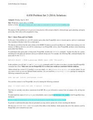
6.830 Problem Set 2 (2009) - MIT Database Group

6.830 Problem Set 2 Solutions 16.830 Problem Set 2 (2009)The purpose of this problem set is to give you some practice with concepts related to schema design, query planning, and queryprocessing.Part 1 - Query PlansWe show two SQL queries over the NSF database used in Problem Set 1 below. For these two queries, you will examine thequery plan that Postgres uses to answer the query, and try to understand why it produces the plan it does.To understand what query plan is being used, PostgreSQL includes the EXPLAIN command. It prints the plan for a query,including all of the physical operators and access methods being used. For example, the following SQL command displays thequery plan for the SELECT:EXPLAIN SELECT name FROM researchers WHERE researchers.name like ’%Madden%’ ;You can run this by first connecting to hancock’s PostgreSQL server withpsql -h hancock.csail.mit.edu -p 5433 6.830-2009 usernameTo understand the output of EXPLAIN, you will probably want to read the performance tips chapter of the PostgreSQL documentation:http://www.postgresql.org/docs/8.3/static/performance-tips.htmlWe have run VACUUM FULL ANALYZE on all of the tables in the database, which means that all of the statistics used byPostgreSQL should be up to date.For the following two queries, answer these questions:a. What physical plan does Postgres use? Your answer should consist of a drawing of a query tree annotated with the accessmethod types and join algorithms.b. Why do you think Postgres selected this particular plan?c. What does Postgres estimate the size of the result set to be?d. When you actually run the query, how big is the result set?e. Run some queries to compute the sizes of the intermediate results in the query. Where do Postgres’s estimates differ fromthe actual intermediate result cardinalities?f. Given the tables and indices we have created, do you think Postgres has selected the best plan? You can list all indiceswith \di, or list the indices for a particular table with \d tablename. If not, what would be a better plan? Why?

6.830 Problem Set 2 Solutions 21. [5 points]: Query 1:SELECT r1.nameFROM researchers AS r1, researchers AS r2, grants, grant_researchers AS grWHERE grants.pi = r2.idAND grants.id = gr.grantidAND gr.researcherid = r1.idAND r1.org = 10AND r1.org != r2.org;Answer:hashindexnested loopsindex scangrants.idseq scan r2hashseq scan grfilter org=10a.seq scan r1b. Working from the bottom up, the query scans/filters r1 because using the index on r1.id would require lots of randomseeks into r1 to test org=10. There’s no predicate on grant researchers so the only choice is to sequentially scan it.Hash join is in general the best choice when there isn’t a need for output in sorted order or an obvious index-basedplan.It is somewhat unclear why it chooses to do an index-nested loops join with the joined ri/gr table and grants – itestimates that it will do 1929 index lookups which sounds expensive relative to building a hash table on the grantstable. This appears to be a bad plan choice.Again, it chooses a hash join for the top-most join, because that’s faster than the random seeks that would berequired to use r2’s index, and a large fraction of r2’s pages will be examined.c. 1586d. 28e. The counts are only wrong in the top-most join (e.g., in the check of r1.org r2.org).f. The plan looks reasonable, except for the choice of index-nested-loops for the middle join.

6.830 Problem Set 2 Solutions 32. [10 points]: Query 2:SELECT r.name, gr.grantidFROM grant_researchers AS gr, grant_programs AS gp, grant_fields AS gf, researchers as rWHERE gr.grantid = gp.grantidAND gr.grantid = gf.grantidAND gr.researcherid = r.idAND gf.fieldid < 200AND gp.programid < 200ORDER BY gr.grantid;Answer:sort on grantidmergehashmergeon gp.grantid = gf.grantida.seq scanresearchersseq scangrindex scangpindex scangfb. This is a very interesting plan. First, it is a bushy plan, which joins gp and gf (using a merge join), gr and r (usinga hash join) and then joins those two results (using a merge join.) Merge joins are selected because they producedata in grantid order. Note that it joins gp and gf, which don’t actually have a join predicate in the above query;surprisingly, the join condition is on gp.grantid = gf.grantid, which is a predicate the system is able to infer fromforeign key relationships and the conditions gr.grantid = gf.grantid and gr.grantid = gp.grantid.Hash join is used between r and gr because hash join is generally the best way to combine two large tables withouta selective predicate between them (as above.) There’s no way to use a sort-merge join for this join to produce thatdata in grantid order. It is somewhat unusual that it chooses to perform this join first – it seems that first producing arestricted version of gr joined with gf and gp and then joining that with r might be more efficient. The sort is neededto get the data in grantid order for the outer merge join.c. 20514d. 14606e. Its estimate of the hash join size is perfect. It slightly overestimates the size of the middle merge join (actual=9986,estimated = 11894.) This probably accounts for the error in its over all estimate of the final join size. In general,this is not a bad estimate of the total cost.f. As noted above, this is a surprisingly sophisticated plan. A better plan might be to first join gf and gp with gr, andthen join that result with r, using a sort merge join, since that would have produced an intermediate table with anestimated 11894 results, instead of the 13496 rows in the original gr table. However, the plan that is chosen seemsreasonable given that this reduction isn’t particularly significant.

6.830 Problem Set 2 Solutions 43. [10 points]:Use EXPLAIN to find the query plans (including access methods types and join algorithms) for the following threequeries, draw the query tree for each of them, and answer the questions below.a. SELECT researchers.orgFROM researchers, grantsWHERE researchers.id = grants.piAND grants.amount > 40000000;Answer:Nested Loop (cost=0.00..16.55 rows=1 width=4)-> Index Scan using gamt on grants (cost=0.00..8.27 rows=1 width=4)Index Cond: (amount > 40000000::double precision)-> Index Scan using researchers_pkey on researchers (cost=0.00..8.27 rows=1 widthIndex Cond: (researchers.id = grants.pi)nested loops joinindex scanon grants.amount > 40000000index scanon reseachers.pkeyb. SELECT researchers.orgFROM researchers, grantsWHERE researchers.id = grants.piAND grants.amount > 3500000;Answer:Hash Join (cost=155.20..1577.00 rows=794 width=4)Hash Cond: (grants.pi = researchers.id)-> Bitmap Heap Scan on grants (cost=18.40..1425.32 rows=794 width=4)Recheck Cond: (amount > 3500000::double precision)-> Bitmap Index Scan on gamt (cost=0.00..18.21 rows=794 width=0)Index Cond: (amount > 3500000::double precision)-> Hash (cost=78.02..78.02 rows=4702 width=8)-> Seq Scan on researchers (cost=0.00..78.02 rows=4702 width=8)hash joinheap scan filtered by bitmap on grantsseq scan onresearchersbitmap index scanon grants.amount > 3500000c. SELECT researchers.orgFROM researchers, grantsWHERE researchers.id = grants.piAND grants.amount > 35000;Answer:

6.830 Problem Set 2 Solutions 5Hash Join (cost=136.79..2134.09 rows=8267 width=4)Hash Cond: (grants.pi = researchers.id)-> Seq Scan on grants (cost=0.00..1842.29 rows=8267 width=4)Filter: (amount > 35000::double precision)-> Hash (cost=78.02..78.02 rows=4702 width=8)-> Seq Scan on researchers (cost=0.00..78.02 rows=4702 width=8)hash joinfilter on grants.amount > 35000seq scan onresearchersseq scan ongrantsa. You may notice that the query plans for the three queries above are different, even though the all have the samegeneral form. Explain in a sentence or two why the plans are different.As the selectivity of the grants predicate changes, different plans become better or worse. For a veryselective predicate, an index scan makes sense since it returns fo sfew results. For a very non-selectivepredicate (in the third case), a hash join is the best choice. In the middle case, Postgres uses somethingcalled a “bitmap heap scan”, which uses the indices to produce a bitmap of records that satisfy thequery without doing a lookup on the heapfile to retrieve the tuples, and then scans the bitmap to retrievesatisfying records. This has better I/O performance than a pure index scan because the accesses to theheapfile are in sequential order rather than being randomly scattered through it.b. More generally, if we’re running the queries above where we vary the constant s after the ’>’, for what value ofs does Postgres switch between the three plans? Why does it decide to switch plans at that value? Please be asquantitative as possible in your explanation.Note that there are actually four plans that the system uses; the one that is missing is an index nestedloops join that also uses the bitmap heap scan. It is only used for a small range of s values between31597642 and 32440920 (plans that are estimated to produce between 27 and 4 tuples.) Its performanceis very similar to the first plan. We’ll call this plan 1a, and the plans above plan 1,2, and 3.It switches from plan 1a to plan 2 at s = 31597641. It is at this point that the estimated number of rowsproduced goes from 27 up to 28, and the cost of the hash join join is estimated to be faster than indexnested loops with an bitmap index scan on grants. The cost of the index nested loops join gets higheras more grants tuples satisfy the condition, leading to more index lookups (and more random I/Os) beingperformed. In constrast, the cost of the building the hash on grants is insensitive to the number of lookups.It switches from the plan 2 to plan 3 at s = 499999. It is at this point that the total cost of the bitmap heapscan exceeds the cost of doing a regular sequential scan (i.e., for s = 500000, the cost of the bitmapheap scan is estimated to be 1810; the cost of the sequential scan is estimated at 1846.) Larger s valuesare estimated to have a lower selectivity and reduced cost when using the bitmap heap scan. Smaller svalues are estimated perform better with a pure hash scan because the cost estimate of using the indexto do the lookup on the outer relation exceeds the cost estimate of sequentially scanning the otuer.

6.830 Problem Set 2 Solutions 6c. Suppose the crossover point (from the previous question) between queries 1 and 2 is s 0 . Compare the actualrunning times corresponding to the two alternative query plans at the crossover point. How much do they differ?Inside psql, you can measure the query time by using the \timing command to turn timing on for all queries. Toget accurate timing, you may also wish to redirect output to /dev/null, using the command \o /dev/null;you can stop redirection just by issuing the \o command without a file name. You may also wish to run each queryseveral times, throwing out the first time (which may be longer as data is loaded into the buffer pool) and averagingthe remaining runs.AnswerSELECT researchers.orgFROM researchers, grantsWHERE researchers.id = grants.piAND grants.amount > 31597642;Time: .816 msSELECT researchers.orgFROM researchers, grantsWHERE researchers.id = grants.piAND grants.amount > 31597641;Time: 3.552 msSELECT researchers.orgFROM researchers, grantsWHERE researchers.id = grants.piAND grants.amount > 500000;Time: 9.48 msSELECT researchers.orgFROM researchers, grantsWHERE researchers.id = grants.piAND grants.amount > 499999;Time: 13.61 msd. Based on your answers to the previous two problems, is s 0 actually the best place to switch plans, or is it anoverestimate/underestimate of the best crossover point? If s 0 is not the actual crossover point, can you estimatethe actual best crossover point without running queries against the database? State assumptions underlying youranswer, if any.The crossover between the two plans appears to be incorrect. The index nested loops based join wouldstill have been a better choice (this is probably because, although the query is estimated to produce 27or 28 results, it only produces 4, resulting in fewer index lookups than estimated.)It is hard to accurately estimate the actual crossover point without knowing the number of index lookupsperformed on researchers at various points, but the crossover point will occur when the cost of buildingthe hash table on researchers is less than the cost of this number of lookups.

6.830 Problem Set 2 Solutions 7Part 2 - Access MethodsBen Bitdiddle is building a database to catalog his extensive wardrobe. Being a computer scientist, he records each item ofclothing, as well as compatible “outfits” which look good together.Ben creates four tables:• A table of clothes called C, with schema and |C| records init,• A table with metadata about outfits in it O, with schema and |O| records init, and• A many-to-many mapping table specifying which clothes are in a particular outfit CO, with schema and |CO| records in it.• A table containing a list of events and the outfit he wore to each E, with schema and |E| records in it.You may assume ints, floats, and timestamps are 4 bytes, and characters are 1 byte. Disk pages are 10 kilobytes. In the followingthree questions, we provide you with a physical database design and a query workload, and ask you to explain why the databasesystem chooses a particular plan or what plan you think the database would select.Ben’s database supports heap files and B+Trees (clustered and unclustered.) Assume that you can have at most one clusteredindex per file, and that the database system has up-to-date statistics on the cardinality of the tables, and can accurately estimatethe selectivity of every predicate. Assume B+Tree pages are 50% full, on average. Assume disk seeks take 10 ms, and the diskcan sequentially read 100 MB/sec.For the queries below, you are given the following statistics:StatisticValueClothing Items Per Outfit 5Outfits Per Clothing Item 20Distinct Types of Clothing 10Distinct Types of Outfits 5Number of Clothing Items |C| 10 6Number of Outfits |O| 4 × 10 6Number of Events |E| 1000First Event 1/1/1990In the absence of other information, assume that attributes values are uniformly distributed (e.g., that there are approximatelythe same number of each type of clothing, etc.)Ben creates an unclustered B+Tree over C.type. He then runs the query SELECT * FROM C WHERE type = ’sock’.He finds that when he runs this query using the EXPLAIN command, the database does not use the B+Tree he just created.

6.830 Problem Set 2 Solutions 84. [5 points]: Why not? What does the database probably do instead? How much more expensive would it be to usethe B+Tree, in terms of total disk I/Os and disk seeks?It most likely does a sequential scan. This is because the selectivity of the ’sock’ predicate is only .2 and theindex is unclustered, so every page will be read multiple times in random order, incurring many seeks.The C table is 158 bytes per record, so each page contains 10000/158 = 64 tuples, and there are a total of15625 pages required to represent 10 6 clothing items.The seqscan will perform 1 random I/O and read all of these pages.The index scan will retrieve 2 × 10 5 tuples, performing that many index lookups. Since the index pages are50% full and each index page holds 10000 / (50 + 4) = 185 keys plus pointers, this will result in scanning of1081 index leaf pages, with a random I/O between each page. We assume top levels of the index fit in RAM.Each of these 2 × 10 5 index lookups results in a random I/O and a page read from the heap file.It is possible that pages of the heap file might all fit in the buffer pool, in which case these heap-file lookupswould only result at most 15625 seeks plus I/Os (it is likely that every page of the heap file will contain at leaston tuple that satisfies the query).So the index-based plan uses 1081 + 15625 =16706 seeks and I/Os in the best case, while the seq scan uses1 seek and 15625 I/Os.

6.830 Problem Set 2 Solutions 9He now runs the following query to find the value of all of his formalwear outfits worn to events since 1999 (note that this querymay include the value of some items of clothing multiple times.)SELECT SUM(value) FROM C,O,CO,EWHERE co cid = cid AND co oid = oidAND e oid = oid AND outfittype = ’formalwear’AND t >= ’1/1/1999’.5. [5 points]: Draw the query plan you think the database would use for this query given that Ben had created a clusteredB+Tree over oid, a clustered B+Tree over cid, a clustered B+Tree over co oid, co cid, and a clustered B+Treeover e oid.These questions turned out to be hard to answer without making some assumption about how much memoryand the types of joins that are available. Here we assume that there is at least enough RAM to build an inmemory hash or to sort a few thousand tuples, and that both merge and hash jons are available.Total seeks (assuming left branch of 500–2500 tuples can fit into memory): 4Total I/Os = 12 + 29412 + 16000 + 16706 = 62132Runtime ~= 6.2sChoose merge because cost of INL would becost of 2500 random I/Os into C or 25 swhereas seq scan of C takes only 1.67 s2500 tuplesMerge joinsort into cid order(assume in memory)158 bytes per record10000/158 = 64 records per pageC10^6 tuples10^6/64 = 16706 pagesSeq scan on CO takes 1.67 sChoose merge because cost of INL would becost of 500 random I/Os into CO or 5 s,whereas seq scan of CO takes only 1.6 s500 tuplesin oid orderMerge joinoid,cid orderCO8 bytes per record10000/8 = 1250 records per page4x10^6 x 5 = 2x10^7 tuples2x10^7/1250 = 16000 pagesSeq scan on CO takes 1.6 s500 tuplesin oid orderfilter on date > 1/1/1999Merge joinoid orderfilter on type = 'formalwear'Choose merge because costof INL would be cost of 500random I/Os into O, or 5 s,whereas seq scan of O takesonly 2.94 soid orderE112 bytes per record10000/112 = 90 records per page1000 records / 90 = 12 pagesSec scan on E accesses .12 MB, taking.0012 sO74 bytes per record,10000/74 = 136 records per page,4x10^6 records / 136 = 29412 pagesSeq scan on O would access 294 MB,taking 2.94 sIt could be preferable to use a hash at the top rather than a sort and a merge.

6.830 Problem Set 2 Solutions 106. [5 points]: Draw the query plan you think the database would use for this query, supposing that only heap files wereavailable. Estimate the cost difference (in terms of total seeks and I/Os) between this plan and the plan above based onB+Trees.Total seeks (assuming left branch of 500–2500 tuples can fit into memory): 4Total I/Os = 12 + 29412 + 16000 + 16706 = 62132Runtime ~= 6.2sHash joinbuild in memorytable on E-O-CO2500 tuples158 bytes per record10000/158 = 64 records per pageC 10^6 tuples10^6/64 = 16706 pagesSeq scan on CO takes 1.67 sHash joinbuild in memorytable on E-O500 tuplesCO8 bytes per record10000/8 = 1250 records per page4x10^6 x 5 = 2x10^7 tuples2x10^7/1250 = 16000 pagesSeq scan on CO takes 1.6 s500 tuplesHash joinbuild in memorytable on EHash joins are best choicewhen tables are unsorted andno indices are availablefilter on date > 1/1/1999filter on type = 'formalwear'oid orderE112 bytes per record10000/112 = 90 records per page1000 records / 90 = 12 pagesSec scan on E accesses .12 MB, taking.0012 sO74 bytes per record,10000/74 = 136 records per page,4x10^6 records / 136 = 29412 pagesSeq scan on O would access 294 MB,taking 2.94 sBoth plans use the same number of I/Os. The cost of the first plan might be slightly less as merge joins should be abit cheaper than hash lookups, and we save the (small) cost of building hash tables on the left branch, but overall it isprobably a wash.7. [5 points]: Now suppose that the indices were not clustered (assume the keys are randomly distributed throughoutthe heap file.) Estimate the cost (in terms of total seeks and I/Os) of a query plan using these indices as the access methodfor each of the tables. Compare this cost to the one for using the clustered indices described in Q5 as the access methodsfor each of the tables.The best plan is the same as the one given in Q6; the unclustered indices are not useful as they require manyI/Os to produce data in sorted order.

6.830 Problem Set 2 Solutions 11Part 3 – Schema Design and Query ExecutionBetty Butcher is building a database to store data about patients she’s treated in her roadside surgery shack. She wants to recordinformation about her patients, their visits to her shack, the treatments she has available, and the treatments her patients havereceived. Specifically, her database has the following requirements:a. It must record each patient’s name, address, and date of birth, and the date of death (something that happens a bit toooften in Betty’s shack.)b. It must record dates that each patient visited the shack, and the treatments they received on each visit. Each patient mayreceive multiple treatments per visit.c. It must record names (e.g., “hacksaw”), types (e.g., “amputation”) , descriptions (e.g., “cut that sucker off”), and perunitcost (e.g., “$100”) of different treatments. Different patients may receive different numbers of each treatment (e.g.,two amputations would be recorded as two-units of ’hacksaw’) and each patient may receive different amounts of eachtreatment on different visits.8. [5 points]: Suggest a set of non-trivial functional dependencies for this database from Betty’s requirements givenabove. You may make additional assumptions when deriving these FDs (e.g., that patients only die or are born once, oraddresses don’t change.)We assume patients only die or are born once, and only live at one address.patientid → patient-name,address,birthday,deathdayTreatments have a constant cost.treatmentid → treatment-name,type,description,costPatients visit once per date.visitid → patientid,dateOn each visit, different amounts of different treatments are given.visitid, treatmentid → amountNot having taken 6.830, Betty isn’t sure how to use FDs to generate a schema, so she decides to make something up. Specifically,she represents her database with two tables; a “patientvisits” table which includes information about a patient and his or hervisits, and a table of “treatments” in which the treatments that were administered are recorded.patientvisits : {pv id | p name | p addr | p bday | p diedon | pv visitdate }treatments : {t id | t visitid REFS patientvisits.pv id| t name | t type | t description | t cost | t amount }In the patientvisits table, a given patient may appear multiple times if he or she has visited the shack repeatedly. Similarlytreatments table includes one row for each treatment a patient receives on each visit.This representation works fine for a few months, but as Betty’s database grows, she finds it is very hard to maintain, particularlyas the popularity of her service grows.9. [5 points]: Based on your functional dependencies, list three problems that Betty’s schema may cause as her databasegrows and is subject to lots of inserts and deletes.1. If a patient dies, the value of died on may need to be changed in multiple records in patientvisits.2. If a treatments cost or description changes, it may need to be updated in many records in treatment.3. If a new patient hasn’t visited yet, pv visitdate would have to be null. After that patient visits for the firsttime, this old entry must be updated to indicate the date of the first visit, or the old entry must be deleted anda new one added.

6.830 Problem Set 2 Solutions 1210. [10 points]: Draw an ER diagram for the data Betty wants to store.amountnamereceiveddescriptionNNdatevisittreatmentNcostvisiteddday1patientbdayaddrname11. [5 points]: Use your ER diagram to derive a normalized schema for Betty’s database. You may want to introducedifferent or additional attributes (e.g., id fields) than those Betty chose to use in her initial schema.patient : {patientid, dday, bday, addr, name}received : {visitid, treatmentid, amount}visited : {visitid, patientid, date}treatment : {treatmentid, name, description, cost}12. [5 points]: Use your functional dependencies to derive a schema in BCNF for Betty’s database.Step 1: We have the relation:R: patientid, patient-name,addres,bday,dday,treatmentid,treatment-name,type,description,cost,visitid,patientid,date,amountUsing FDpatientid → patient-name,address,birthday,deathdaywe decompose R to get:A: patientid, patient-name,address,birthday,deathday (this is in BCNF)andB: patientid,treatmentid,treatment-name,type,description,cost,visitid,patientid,date,amount (not in BCNF)Step 2: We decompose B using FD:treatmentid → treatment-name,type,description,costto get:C: treatmentid,treatment-name,type,description,cost (in BCNF)andD: patientid,treatmentid,visitid,patientid,date,amount (not in BCNF)

6.830 Problem Set 2 Solutions 13Step 3: We decompose D using FD:visitid → patientid,dateto get:E: visitid,patientid,date (in BCNF)andF: treatmentid,visitid,amount (also in BCNF)F is in BCNF because it is implied by the FD visitid, treatmentid → amountIn the end, we have four relations:A: {patientid, patient-name,address,birthday,deathday}C: {treatmentid,treatment-name,type,description,cost}E: {visitid,patientid,date}F: {treatmentid,visitid,amount}13. [2 points]: Are the two representations you derived equivalent? If not, in what way do they differ?Both representations are equivalent.14. [3 points]: Do both schemas address the three problems you listed above? Do they both preserve all of the functionaldependencies you gave?Both address all three problems. Both preserve all functional depedencies.