Calibration

Calibration 

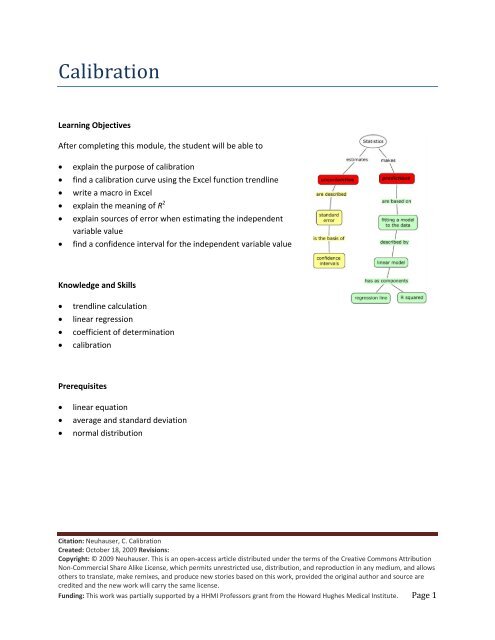
Learning Objectives 

After completing this module, the student will be able to 

• explain the purpose of calibration 

• find a calibration curve using the Excel function trendline 

• write a macro in Excel 

• explain the meaning of R 2 

• explain sources of error when estimating the independent 

variable value 

• find a confidence interval for the independent variable value 

Knowledge and Skills 

• trendline calculation 

• linear regression 

• coefficient of determination 

• calibration 

Prerequisites 

• linear equation 

• average and standard deviation 

• normal distribution 

Citation: Neuhauser, C. Calibration 

Created: October 18, 2009 Revisions: 

Copyright: © 2009 Neuhauser. This is an open‐access article distributed under the terms of the Creative Commons Attribution 

Non‐Commercial Share Alike License, which permits unrestricted use, distribution, and reproduction in any medium, and allows 

others to translate, make remixes, and produce new stories based on this work, provided the original author and source are 

credited and the new work will carry the same license. 

Funding: This work was partially supported by a HHMI Professors grant from the Howard Hughes Medical Institute. Page 1

Pre‐assessment 

Before completing the module test whether you master the prerequisites. Linear Equation 

1. Find the equation of a horizontal line that goes through the point (2,4). 

2. Find the equation of a vertical line that goes through the point (‐1,3). 

3. Determine the equation of the line passing through (‐2,1) and (3,‐1/2). 

4. Determine the equation of the line passing through (1,‐2) and (‐2,4). 

5. Determine the equation of the line with slope 3 and vertical intercept (0,2). 

6. Determine the equation of the line passing through (‐1,‐1) and parallel to the line passing through 

(0,1) and (3,0). 

7. Graph of the line given by the equation y= 2x + 1. 

8. Graph the line given by the equation 3x − 4y + 1= 

0. 

Average and Standard Deviation 

9. Find the average and sample standard deviation of the following data set: 2,4,5,6,6,7,8 

10. Write down the equation for calculating the average and the sample standard deviation of a data set 

of size n: x1, x2,..., x 

n 

Normal Distribution 

11. Suppose X is normally distributed with mean 2 and standard deviation 1. Find (a) the 75 th percentile, 

(b) the 95 th percentile, and (c) the 99 th percentile. 

12. Suppose X is normally distributed with mean 3 and variance 4. Find the probability that X is between 

1 and 4, that is, find P(1 ≤ X ≤4) 

. 

13. Suppose X is normally distributed with mean ‐1 and standard deviation 4. Find an interval centered 

about the mean so that with probability 0.95 X is contained in that interval. 

14. Suppose that the number of seeds a plant produces is normally distributed with mean 142 and 

standard deviation 31. Find the probability that a randomly sampled plant will produce more than 

200 seeds. 








Calibration 

According to the NIST handbook 

(http://www.itl.nist.gov/div898/handbook/pmd/section1/pmd133.htm), “[t]he goal of calibration is to 

quantitatively convert measurements made on one of two measurement scales to the other 

measurement scale.” The relationship between two measurements is used to convert one measurement 

into the other measurement. You saw one such example in your chemistry lab where you measured 

absorbance to find the concentration of an unknown sample. In this case, the relationship between 

absorbance and concentration was linear. You derived the relationship by measuring absorbance of 

standard samples of known concentration. The resulting line is called calibration curve. The basis for the 

calibration curve is Beer’s Law, which states that there is a direct linear relationship between 

absorbance (A) and concentration (c): When if we graph absorbance as a function of concentration, a 

straight line with positive slope provides a good fit. To illustrate this, we provide in the following table 

absorption measurements of standard samples: 

Concentration Absorbance 

[μmole L ‐1 ] 

0 0 

20 0.2356 

40 0.4725 

60 0.7127 

80 0.9507 

If we graph the data points and fit a straight line through the points (Figure 1), we find that the equation 

of the straight line is A= 0.0119c− 0.0014 . 

Figure 1: Straight line fit 








This curve is called a standard curve and is used to infer the unknown concentration of a solution. For 

instance, if we find that the absorbance A of an unknown solution is 0.6386, we find for the 

concentration c 

0.6386 −− ( 0.0014) 

c = = 53.8 

0.0119 

The data in our example fits Beer’s Law extremely well. The data was generated using a Virtual Lab on 

Spectrophotometry (http://www.chm.davidson.edu/vce/Spectrophotometry/UnknownSolution.html). 

When data are obtained in actual lab experiments, measurement errors need to be taken into account. 

A Model for Linear Calibration 

We assume in the following that we measure a signal y that depends linearly on a quantity x. We call the 

quantity x the independent variable and the quantity y the dependent variable. We assume that we 

measure x without error and that the quantity y is measured with an error ε that is normally distributed 

with mean 0 and standard deviation σ. The relationship between the two quantities is then 

y= a+ bx+ 

ε 

To get a sense for the measurement uncertainty when inferring the quantity x from the measurement y, 

we begin with simulating an experiment in which we have a set of n standard samples and for each 

sample we measure the signal m times. 

In‐class Activity 1 

In the spreadsheet CalibrationWorkbook under the tab “Simulation,” you will find the simulation of 

standard samples with values x = 10,20,40,60,80 and 90 and where the intercept a = 0 and the slope 

b = 1. Each signal is measured 3 times. The simulated data are in the gray‐colored box. The input 

parameters for the slope, the intercept, and the standard deviation s.d. for the error are in the yellowcolored 

box. The trendline is calculated using the Excel function LINEST. (This function is difficult to use 

and you will not need to learn how at this point.) 

To investigate how the estimated value of the independent variable x depends on the error ε, we 

proceed as follows. We assume that the (unknown) value of the independent variable x is equal to 50 








(Cell F11). Using the equation y= ax+ b+ ε with a = 1 and b = 0 with s.d. 1, we can calculate the 

measured value of the quantity y (Cell F12). We can then use the estimated trendline to find the 

estimate for x (Cell F13) . The graph displays the simulated data from the calibration experiment, the 

trendline, and the data point corresponding to the unknown sample. 

When you press F9, you will see that Excel runs another simulation. By repeatedly pressing F9, you can 

get a sense for the variability of the estimated value of x in our simulation experiment. It is tedious to 

record manually the values of repeated simulations. Excel has a feature, called Macro, that records 

repeated key strokes. Let’s write a macro to record the outcome of repeated simulations for the 

estimate of x. 

(a) To write a macro to simulate values of x, proceed as follows: 

1. Open the Developer tab and click on Record Macro in the Code group. 

2. Give the macro a name and select a key, for instance, Ctrl‐a works. 

3. Select the Home tab. 

4. Copy the value of x from Cell F13. 

5. Paste the value of x into Cell Q3 as Paste Value. 

6. Click on Insert in the Cells group and click on Shift cells down in the Insert window. 

7. Go to the Developer tab and click on Stop Recording in the Code group. 

If you press Ctrl‐a, the simulated values will be copied into your spreadsheet in Column Q. Repeat the 

simulation 100 times. (The numbers in Column P help you keep track of the simulations.)Sort the 

simulated values from Smallest to Largest. Find the middle 90%. 

(b) Repeat the simulation when x = 15 . Are the inferred values of x more or less spread out compared 

to when x = 50 

(c) Change the standard deviation to see how an increase/decrease in the measurement error affects 

the uncertainty in the calculation of x. 








Figure 2: Screenshot of the simulation. The input parameters are listed in the yellow box; the simulated data are 

listed in the gray box; the estimated values of the slope and vertical intercept are listed in the green box together 

with the calculation of the unknown quantity x based on the measurement of the unknown sample y. The graph 

displays the simulated data (blue symbols), the trendline (black line), and the unknown measurement (red data 

point). 

Linear Regression 

When two quantities are linearly related, such as absorbance and concentration, a straight line provides 

a good fit. In Excel, a straight line can be fitted using the Trendline option. The Trendline option is under 

the Layout in the Chart Tools. When clicking on the blue triangle under Trendline and choosing More 

Trendline Options, a window opens that offers additional options, such as Display Equation on chart 

and Display R‐squared value on chart. We already know the meaning of the Equation. We will now look 

at the meaning of R‐squared. 

Assume a linear model y= a+ bx+ ε where the error has mean 0 and standard deviation σ . We 

obtained data points ( x , y ), j= 1,2,..., n, and used the Trendline option to fit a straight line. This results 

j 

j 

in estimates for the slope and the intercept. We denote the estimated value of the intercept by â and 

the estimated value of the slope by ˆb. 








How does Excel estimate the slope and the intercept 

The method that Excel uses to estimate the slope and the intercept is called method of least squares. 

The method says: Find â and ˆb so that the expression 

n 

∑ 

j= 

1 

⎡y ( ˆ ˆ 

j 

− a+ 

bxj) 

⎤ 

⎣ ⎦ 

2 

is as small as possible. We say that the sum of the squared deviations is minimized. Expressions for the 

estimated intercept and slope can be given. It is not important to memorize the expressions. 

The least square line (or linear regression line) is given by 

with 

bˆ 

= 

∑ 

y= aˆ 

+ bx ˆ 

n 

j= 

1 j 

n 

∑ j= 

1 

aˆ 

= y −bx 

ˆ 

( x − x)( y − y) 

2 

( x − x) 

j 

j 

To measure how good the fit is we calculate a quantity called the coefficient of determination, which is 

abbreviated as R 2 . For each data point ( x , y ), we can define y = aˆ 

+ bx ˆ . We introduce the deviation of 

the measured y‐values from their mean, 

j 

yj 

j 

− y 

ˆ j 

, which we can write as 

y − y = ( y − yˆ 

) + ( yˆ 

− y) 

j j j j 

n 

2 

A somewhat lengthy calculation shows that the total sum of squared deviations ∑ ( y ) 

j 1 j 

− y can be 

= 

written as a part that is explained by the linear model (Explained) and a part that reflects the stochastic 

errors (Unexplained) 

j 

n n n 

2 2 2 

( y ) ( ˆ ) ( ˆ 

j 

− y = yj − y + yj −yj) 

j= 1 j= 1 j= 

1 

∑ ∑ ∑ 

 

Total Explained Unexplained 

The ratio between the explained variation and the total variation is the coefficient of determination 








R 

2 

∑ 

∑ 

2 

Explained ( yˆ 

) 

1 j 

− y 

j= 

= = 

n 

Total 2 

( y − y) 

n 

j= 

1 

j 

The coefficient of determination 

2 

R is the proportion of variation that is explained by the model. 

In‐class Activity 2 

Return to the spreadsheet CalibrationWorkbook. Under the tab “Simulation,” you have already worked 

on the simulation of standard samples with values x = 10,20,40,60,80 and 90 and where the intercept 

a = 0 and the slope b = 1. Each signal is measured 3 times. The simulated data are in the gray‐colored 

box. The graph has a small textbox where the equation of the trendline and the coefficient of 

determination is listed. You will see that when you increase the standard deviation, the coefficient of 

determination decreases. Give a verbal explanation as to why you would expect this. 

The Chemistry Calibration Lab 

In your Calibration Lab, you were asked to prepare a calibration curve. The spreadsheet 

CalibrationLab.xlsx will help you do the analysis. Open the spreadsheet. The Calibration Lab Analysis 

sheet is set up so that you can enter your data into the yellow cells. To calculate the calibration curve, 

enter the data from the absorbance measurements of the standard samples into C4:C21 (Step 2). The 

spreadsheet will calculate the slope and intercept in the cells I19 and I20, respectively, (see blue cells 

and Step 3). In Step 4, the spreadsheet calculates the coefficient of determination. Compare the values 

in the cell to the textbox in the figure that has the same information. 

(a) To include the uncertainty of the calibration curve in your lab report, record the coefficient of 

determination together with the equation of the trendline. Explain in words the meaning of the 

coefficient of determination. 

(b) In the chemistry lab, you then determined the concentration of an unknown sample based on the 

calibration curve. Enter the three measurements into cells B25‐B27 (Step 5). The spreadsheet is set up 

so that it calculates the estimated concentration. Use paper and pencil to verify the result in Cell B 31 

(estimated concentration) the spreadsheet. 

(c) While the theory is beyond this course, the spreadsheet is set up to calculate a confidence interval 

for the estimated concentration * x . In Cell K25, you can set the confidence level, for instance 95%. The 

lower and upper limits of the confidence interval are listed in Cells K27 and K28, respectively. Record the 








confidence interval. The Cell K26 contains the value of half the length of the confidence interval, which 

we denote by C 

x . We can thus report the result also as x* ± Cx 

. 

If you want to read more about Linear Calibration, consult the statistics and data analysis paper by 

Burke, S. Regression and Calibration. LC GC Europe Online Supplement. 

Homework 

1. Find a linear regression line through the given points and compute the coefficient of determination 

x ‐3.0 ‐2.0 ‐1.0 0.0 1.0 2.0 

y ‐6.3 ‐5.6 ‐3.3 0.1 1.7 2.1 

2. To determine whether the frequency of chirping crickets depends on temperature, the following 

data were obtained by Pierce, 1949 (The Songs of Insects. Cambridge, Mass. Harvard University 

Press): 

Temperature (F) 69 70 72 75 81 82 83 84 89 93 

Chirps/sec 15 15 16 16 17 17 16 18 20 29 

Fit a linear trendline and find the coefficient of determination. 

3. To determine the glucose in a wine sample an enzyme spectroscopy method is used. The calibration 

curve is obtained from the following data 

Added glucose, 0.000 0.050 0.100 0.200 0.300 0.400 

[glucose] (mM) 

Absorbance 0.231 0.279 0.314 0.423 0.540 0.665 

(a) Find the equation of the calibration curve and the coefficient of determination. 

(b) Suppose the absorbance of an unknown sample is measured as 0.356. Use the calibration curve 

to estimate the glucose level.

Calibration

Create successful ePaper yourself

Delete template?

Save as template?