Detecting the long-term impacts from climate variability and ... - HAL

Hydrol. Earth Syst. Sci., 10, 703–713, 2006
www.hydrol-earth-syst-sci.net/10/703/2006/
© Author(s) 2006. This work is licensed
under a Creative Commons License.
Hydrology and
Earth System
Sciences
Detecting the long-term impacts from climate variability and
increasing water consumption on runoff in the Krishna river basin
(India)
L. M. Bouwer 1 , J. C. J. H. Aerts 1 , P. Droogers 2 , and A. J. Dolman 3
1 Institute for Environmental Studies, Faculty of Earth and Life Sciences, Vrije Universiteit, Amsterdam, The Netherlands
2 FutureWater, Wageningen, The Netherlands
3 Department of Hydrology and Geo-environmental Sciences, Faculty of Earth and Life Sciences, Vrije Universiteit,
Amsterdam, The Netherlands
Received: 6 March 2006 – Published in Hydrol. Earth Syst. Sci. Discuss.: 4 July 2006
Revised: 5 September 2006 – Accepted: 26 September 2006 – Published: 4 October 2006
Abstract. Variations in climate, land-use and water consumption
can have profound effects on river runoff. There
is an increasing demand to study these factors at the regional
to river basin-scale since these effects will particularly
affect water resources management at this level. This
paper presents a method that can help to differentiate between
the effects of man-made hydrological developments
and climate variability (including both natural variability and
anthropogenic climate change) at the basin scale. We show
and explain the relation between climate, water consumption
and changes in runoff for the Krishna river basin in central
India. River runoff variability due to observed climate variability
and increased water consumption for irrigation and
hydropower is simulated for the last 100 years (1901–2000)
using the STREAM water balance model. Annual runoff under
climate variability is shown to vary only by about 14–34
millimetres (6–15%). It appears that reservoir construction
after 1960 and increasing water consumption has caused a
persistent decrease in annual river runoff of up to approximately
123 mm (61%). Variation in runoff under climate
variability only would have decreased over the period under
study, but we estimate that increasing water consumption has
caused runoff variability that is three times higher.
1 Introduction
Human induced climate change, as well as natural climate
variability, may have profound impacts on freshwater resources
in many areas (Arnell et al., 2001). However, these
impacts may be obscured by non-climatic factors, often an-
Correspondence to: L. M. Bouwer
(laurens.bouwer@ivm.falw.vu.nl)
thropogenic in origin. Therefore, the relative impact of climate
compared to non-climatic factors is important when
studying the relation between climate and water resources
availability. Non-climatic factors may be land use and land
cover change. In particular developments in water storage in
reservoirs and consumption for irrigation and industry cause
increased evaporation and substantial effects on river runoff
(e.g. Döll and Siebert, 2002; De Rosnay et al., 2003; Haddeland
et al., 2006). Water consumption may affect the annual
water budget, while the structures that capture water such as
dams and reservoirs may change the patterns of the annual
hydrological cycle. The global amount of water consumed
for agriculture has been estimated to have roughly doubled
between 1900 and 1980 (Falkenmark and Lannerstad, 2005).
Water has therefore been identified a critical factor for reaching
the Millennium Development Goals (Rockström et al.,
2005), and further assessment of shifts in water availability
is needed.
Several studies have been devoted to either the impact of
climate conditions or environmental and human use of water
availability. Using hydrological models, it is possible
to make a distinction between pristine catchment conditions
and the effects of environmental changes (e.g. Letcher et al.,
2001). Recent global studies on the effects of water storage
and consumption have shown dramatic effects on the frequency
of low flows and downstream water resources and
services (Syvitski et al., 2005; Nilsson et al., 2005). Examples
include the reduction of the amount of total river
runoff, the reduction in peak flow intensity, reduction in sediment
transport, and changes in water quality, with consequences
for downstream river morphology and ecology. Regional
studies show similar trends. For instance, Magilligan
et al. (2003) estimated that the peak discharges occurring every
two years have decreased by about 60% for a number
Published by Copernicus GmbH on behalf of the European Geosciences Union.

704 L. M. Bouwer et al.: Long-term impacts from climate and water consumption
Mumbai
Pune
Hidkal
Koyna
Manikdoh
Ujjani
Krishna river
Tungabhadra
Bhima river
Bhadra
Mangalore
Hyderabad
Nagarjuna Sagar
Sri Sailam
Tungabhadra river
0 100 Kilometers
Bangalore
Vijayawada
India
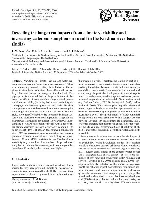
Fig. 1. Map of the Krishna river basin with its main tributaries, major
cities (squares) and the discharge gauging station at Vijayawada
(triangle) at the lower end of the river. The open circles indicate the
locations of the eight largest reservoirs in the basin.
of river basins in the United States. Schreider et al. (2002)
showed that due to the construction of small farm dams in
Australia small but detectable changes can occur in the daily
discharges. It has thus been argued that natural processes are
no longer the sole influence on river systems: anthropogenic
influences currently dominate (Meybeck, 2003).
Some researchers have approached these anthropogenic
influences by using the green- and blue water concept. Green
water refers to the amount of available freshwater that is used
for evaporation in natural or agricultural vegetation, which is
consumptive use, whereas blue water refers to the amount
of water that is unaffected or remains as return flow. The
blue water flow is important for downstream water availability,
and it has been proposed that a certain requirement for
minimum flow exists for ecological sustainability (Tharme,
2003). However, while an assessment of “green” and “blue”
water flows is important for proper decisions in water resources
management, the total amount of available freshwater
from which allocations can be made is not constant over
time, mostly because of variations in climate. It appears,
however, that very few studies pay attention to the combined
effect of natural climate variability, climate change and anthropogenic
impacts (e.g. Changnon and Demissie, 1996). It
also happens that studies on water availability have used relatively
short time intervals or concentrate on the average climate
state and effects at the global or regional scale (e.g. Alcamo
et al., 1997). Vörösmarty et al. (2000) compared the
impacts from climate change and population growth and concluded
that average climate change is likely to have a minor
impact on water resources. However, they ignored the potential
impacts that changes in year-to-year variability of climate
may have. Most climate trend detection analyses so
far have focussed on the analysis of the mean river runoff
and not on changes in runoff variability (for an overview see
Kundzewicz and Robson, 2004). The assessment of historic
high and low flows as demonstrated by Burn and Hag Elnur
(2002), or statistical analyses applied to climate change scenarios
as demonstrated for low flows by Arnell (2003), have
shown the impact of climate variability on the variability of
river runoff. Studies of runoff effects caused by both climate
variability and basin developments should consider long and
discrete periods, preferably more than 50 years in order to
capture multi-decadal variability of climate and river runoff.
The main goal of the present research was to develop and
test a method to separate the relative impact of observed climate
variability (which in this study is defined to include
both natural variability and anthropogenic climate change)
versus human water use on river runoff variability at the
river basin scale. We have limited ourselves to studying the
impacts of increasing water consumption for irrigation and
evaporation losses from water storage for hydropower production
on the annual and seasonal river runoff over a period
of 100 years. These factors were studied in the arid region
of the Krishna river basin, which is located in central India.
The objectives of this study were to:
– Assess and present statistics of the variation in climate
and river discharges, in particular changes in precipitation
and annual river runoff;
– Calibrate and validate a spatial hydrological model in
order to simulate monthly river runoff over a 100-year
period under climate variability, with and without accounting
for changes in water consumption;
– Quantify changes in annual and seasonal river runoff
and runoff variability over 100 years by comparing observed
and modelled monthly river runoff;
– Determine the relative influence of variation in climate
versus increasing water consumption on annual basin
river runoff and runoff variability.
2 Study area and data
2.1 The Krishna river basin
The Krishna river basin is the second largest river
in peninsular India and stretches over an area of
258 948 km 2 . The basin is located in the states of Karnataka
(113 271 km 2 ), Andhra Pradesh (76 252 km 2 ) and Maharashtra
(69 425 km 2 ). The basin represents almost 8% of surface
area of the country of India and is currently inhabited
by 67 million people. The major tributaries of the river include
the Bhima River in the north and the Tungabhadra
River in the south (Fig. 1). The river terminates at the Krishna
delta in the Bay of Bengal. The climate in the basin
is characterised by sub-tropical conditions with considerable
Hydrol. Earth Syst. Sci., 10, 703–713, 2006
www.hydrol-earth-syst-sci.net/10/703/2006/

L. M. Bouwer et al.: Long-term impacts from climate and water consumption 705
rainfall in the mountains of the Western Ghatts and arid conditions
in the basin interior. Total annual rainfall today averages
835 mm, while the annual average temperature reaches
26.7 ◦ C. Rainfall over India is highly variable due to the intraseasonal
and inter-annual variability of the South-West monsoon
(June to September) and the North-East monsoon (October
to November), leading to alternating drier and wetter
conditions on the Indian continent (Krishnamurthy and
Shukla, 2000; Munot and Kothawale, 2000). A dry season
occurs during the period December–May.
Failing monsoons have often resulted in considerable declines
in water availability and consequently led to increasing
political tensions between the states. One of the driest recent
episodes in Central India occurred in 1972 (see Fig. 2).
Over 100 million people in India were affected as crops failed
(http://www.em-dat.net). In 1973 the water allocation between
the three riparian states of Maharashtra, Karnataka and
Andhra Pradesh was settled in a water disputes act. Declines
in water availability also impact on water quality. Chloride
concentrations in the Krishna River, for instance, are highly
correlated to total amounts of river runoff (Sekhar and Indira,
2003). It has also been shown that sediment loads of the Krishna
River have decreased over time (Ramesh and Subramania,
1988).
For many centuries small reservoirs, locally known as
tanks, have been constructed to conserve and utilise water,
and under British rule new canals were created, old tanks restored
and new tanks built (Wallach, 1985). But the major
reservoirs and canal systems now present in the basin were
constructed during the second half of the 20th century for
irrigation purposes and hydropower generation. Since the independence
of India in 1947 the construction of reservoirs
started to take off rapidly (Wallach, 1984). All large reservoirs
with a storage capacity of more than 10 9 m 3 were built
after 1953. The locations of the eight largest reservoirs in
the basin are depicted in Fig. 1. These reservoirs were constructed
between 1953 and 1988, and together they account
for 26.6 10 9 m 3 or 80% of the capacity of large reservoirs
in the basin. The storage capacity in the Krishna river basin
is exceeded in India only by the capacity in the Ganges river
basin. The benefits of water storage and redirection are clear:
the current area of land that is being irrigated amounts to
about 3.2×10 6 ha and a total of 1947 MW of electricity is
produced annually.
2.2 Climate and river runoff data
Climate data were retrieved from the global TS 2.0 dataset
from the Climatic Research Unit, which covers the entire
world for the period 1901–2000 on a 0.5 by 0.5 degree grid
(Mitchell and Jones, 2005). Although this climate data has
not been corrected for ambient factors, such as urban development
or land use change, it is the most comprehensive climate
dataset presently available and previous versions have
often been used for studying the hydrological cycle.
anomaly [ C]
º
anomaly [mm]
1.5
1.0
0.5
0.0
-0.5
-1.0
1901 1911 1921 1931 1941 1951 1961 1971 1981 1991 2000
400
300
200
100
0
-100
-200
a
-300
1901 1911 1921 1931 1941 1951 1961 1971 1981 1991 2000
Fig. 2. Temperature (top) and precipitation (bottom) anomalies and
their seven-year moving averages in the Krishna River Basin, relative
to the period 1901–1915. In the lower graph, a and b designate
a dry and a wet year, for which the spatial patterns of effective precipitation
are plotted in Fig. 5.
Data on average monthly river discharges were taken from
the RivDIS database available at http://www-eosdis.ornl.
gov/rivdis/STATIONS.HTM (Vörösmarty et al., 1998) for
the downstream station at the city of Vijayawada (Global
Runoff Data Centre station number 2854300) close to the
mouth of the river; see Fig. 1. The data covers the period
1901–1979, with no data during the period 1961–1964 and
for the year 1975. Additional discharge data for the period
1989–1999 were collected from yearbooks of the Indian Central
Water Commission.
3 Trends in climate, peak runoff and reservoir development
The climate data, discharge data and data on reservoir construction
were investigated in order to assess what determines
the runoff of the Krishna river basin. We considered periods
of 15 years in order to be able to determine changes between
a number of coherent climatic periods.
In Fig. 2 the temperature and precipitation anomalies in the
Krishna river basin are given as deviations from the 15-year
period of 1901–1915. During this period the average annual
total amount of precipitation was 765 mm, while the average
annual temperature was equal to 26.0 ◦ C. Variations between
years and decades can clearly be observed. The data indicates
that the average annual temperature increased by about
0.7 ◦ C, from 26.0 ◦ C over the period 1901–1915 to 26.7 ◦ C
b
www.hydrol-earth-syst-sci.net/10/703/2006/ Hydrol. Earth Syst. Sci., 10, 703–713, 2006

3
reservoir storage [10 m]
9 3
706 L. M. Bouwer et al.: Long-term impacts from climate and water consumption
40
35
500
discharge [10 m s ]
3 -1
30
20
10
30
25
20
15
10
5
total annual runoff [mm]
400
300
200
100
observed
simulated
0
0
1894 1904 1914 1924 1934 1944 1954 1964 1974 1984 1994 2000
Fig. 3. Annual downstream peak discharge values (daily) over the
period 1894–1999 (line), its seven-year moving average and the
cumulative reservoir storage capacity (shaded area) of reservoirs
larger than 10 9 m 3 in the Krishna river basin over the period 1894–
2000. Peak discharge data were obtained from Rodier and Roche,
1984; Herschy, 2003; updated with CWC data for 1996–1999.
over the period 1986–2000. Average total annual precipitation
increased slightly, by 9% between the same periods,
from 765 to 835 mm.
Observed discharge data were converted from cubic metre
per second into runoff in millimetres per month, using the
basin size as reported by Vörösmarty et al. (1998). The storage
capacity of reservoirs larger than 10 6 m 3 has increased
considerably after 1953, as can be seen from Fig. 3. The
major reservoirs in the basin account for a storage capacity
of 34.5×10 9 m 3 . An additional volume is present in numerous
smaller tanks and barrages spread out over the area. The
height of the annual peak discharge has decreased from about
1969 onward; when the seven-year moving average of the
peak discharge drops below the long-term minimum (Fig. 3).
The decreased downstream river runoff coincides with the
rapid increase in reservoir storage capacity during the 1950s
and 1960s.
4 Estimating changes in monthly runoff
From Figs. 2 and 3, the question arises of how much water
would have been available without reservoir development,
and what difference between present and a hypothetical pristine
situation in monthly and seasonal river runoff can be
detected. For these purposes, a water balance model was
developed to simulate monthly river runoff under observed
climate variability and changes in water consumption. Variations
of monthly and seasonal river runoff are important for
the planning and management of agriculture, irrigation and
hydropower production.
4.1 The STREAM model
The STREAM model (Aerts et al., 1999) is a spatial water
balance model based on the formulation of the RHINE-
FLOW model (Van Deursen and Kwadijk, 1993). This model
maximum monthly runoff [mm]
0
1901 1911 1921 1931 1941 1951 1961 1971 1981 1991 2000
150
100
50
observed
simulated
0
1901 1911 1921 1931 1941 1951 1961 1971 1981 1991 2000
Fig. 4. Simulation model results for the period 1901–2000 compared
to the observed total annual river runoff (top) and maximum
monthly river runoff (bottom).
calculates water availability and river runoff on the basis of
temperature and precipitation data and a number of land surface
characteristics. Other factors that may influence in particular
evaporation, such as radiation, wind speed and humidity,
are not included in the model. Radiation is included
indirectly through temperature. The STREAM model for
the Krishna river basin uses geographical information system
(GIS) data at a spatial resolution of 3 by 3 km and at a
monthly time-step. Although the climate data has a lower
spatial resolution, some of the other input data has a finer
resolution (soil water holding capacity and land-use types;
see Appendix A). The water balance is calculated for each
grid-cell using a direct runoff, soil water and groundwater
component (see Appendix A). The STREAM model has been
successfully applied in various forms for climate and hydrology
studies in a number of river basins with similar size and
characteristics as the Krishna river basin (Van Deursen and
Kwadijk, 1994; Aerts et al., 1999; Aerts et al., 2000; Middelkoop
et al., 2001; Winsemius et al., 2006). These studies
have confirmed that a monthly time step is sufficient for detecting
decadal, inter-annual and seasonal changes in the hydrological
cycle, such as those caused by water consumption
and climatic change. The spatial resolution of 3 by 3 km is
sufficient to analyse large-scale patterns, as the basin is approximately
260 000 km 2 in size and since the climate data is
limited to a spatial resolution of 0.5 by 0.5 degrees.
Hydrol. Earth Syst. Sci., 10, 703–713, 2006
www.hydrol-earth-syst-sci.net/10/703/2006/

L. M. Bouwer et al.: Long-term impacts from climate and water consumption 707
Table 1. Observed average amount of annual precipitation and its coefficient of variation, observed and simulated total average annual river
runoff (in millimetres), their standard deviations (SD), coefficients of variation (CV) and model efficiency coefficients (R 2 ) for the different
periods. n designates the number of months that were used to calculate the CV and R 2 of the runoff.
Period 1901–1915 1916–1930 1931–1945 1946–1960 1965–1979 1989–1999
Mean precipitation [mm] 765 737 786 865 798 847
SD [mm] 138 148 116 105 115 72
CV 0.18 0.20 0.15 0.12 0.14 0.08
Mean runoff Observed [mm] 208 213 207 255 120 80
Simulated [mm] 208 178 207 250 205 204
Observed SD [mm] 53 62 42 59 44 43
Observed CV 0.25 0.29 0.20 0.23 0.37 0.53
Simulated SD [mm] 85 80 61 76 60 49
Simulated CV 0.41 0.45 0.29 0.30 0.29 0.24
R 2 0.73 0.68 0.71 0.73 –0.14 –2.74
n 180 180 180 180 168 144
Mean peak runoff Observed [mm] 77 71 68 88 50 35
Simulated [mm] 83 60 72 97 79 75
4.2 Calibration and validation
1972 1988
0
First, the model was calibrated and validated. We assumed a
baseline period between 1901 and 1915 for which the model
was calibrated. Periods of 15 years were chosen, as this
leaves a number of periods before the 1960s (after which major
reservoirs were built) for which the model performance
can be assessed. The calibration of the model involved the
adjustment of a reduction factor that tunes the reference
evaporation (see Eq. A5), a coefficient that determines the
separation between groundwater and runoff (Eq. A2), and a
recession coefficient that determines the delay of the groundwater
flow (Eq. A4). The calibration involved the match to
observed total annual river runoff, as well as seasonal patterns.
The performance of the model was tested at every
stage using the efficiency coefficient R 2 from Nash and Sutcliffe
(1970). After the model was calibrated for the period
1901–1915, the following five 15-year periods for which observed
data were available were used to validate the model.
The model was able to closely match the observed average
annual river runoff (see Table 1). The model results for the
period 1901–2000 are shown in Fig. 4, together with the observed
runoff. By comparing the observed runoff with the
simulated runoff for the remaining 15-year periods the model
performance was assessed. The model efficiency coefficient
after calibration of R 2 =0.73 for the period 1901–1915 indicates
that the model is capable of reasonably estimating
mean monthly runoff for a total of 180 months, in particular
when taking into account the high degree of human intervention
in the hydrological cycle in this basin. Already during
the period 1901–1915 many (small) reservoirs are present
in the basin. The coefficient of determination (r 2 ) between
observed and simulated monthly runoff is 0.77 for the pe-
576
1152
1727
2303 mm
Fig. 5. Effective precipitation over the Krishna river basin for the
years 1972 and 1988.
riod 1901–1915 (n=180) and 0.75 for the period 1901–1960
(n=720). The efficiency coefficient R 2 =0.68 for the period
1916–1930 is slightly lower than the coefficient for the calibration
period (Table 1), but the performance of the model
for the two following periods (1931–1945 and 1946–1960)
is sufficient to assume the model is accurately describing the
runoff during these periods (R 2 =0.71 and R 2 =0.73 respectively).
During the last two simulated periods (1965–1979
and 1989–1999) the fit of the model to the observed data is
not good, as can be seen from the negative model efficiency
coefficients in Table 1.
Annual maximum monthly river runoff is approached reasonably
only in absolute terms for the period 1901–1960,
as can be seen from Fig. 4 (bottom); the coefficient of determination
(r 2 ) between observed and simulated maximum
runoff is only 0.25 for the period 1901–1960. The simulations
of 1960 and beyond act as a reference to detect the
changes in the hydrological cycle. The supposed reason for
the discrepancy is a result of the fact that certain changes,
such as the construction reservoirs, are not captured by the
simulation.
www.hydrol-earth-syst-sci.net/10/703/2006/ Hydrol. Earth Syst. Sci., 10, 703–713, 2006

708 L. M. Bouwer et al.: Long-term impacts from climate and water consumption
Table 2. Top five of simulated annual effective precipitation (defined as precipitation minus actual evaporation) averaged over the Krishna
river basin.
Driest
Wettest
Year Effective precipitation [mm] Year Effective precipitation [mm]
1918 97 1903 546
1972 97 1956 525
1920 98 1975 489
1985 141 1916 472
1987 142 1964 453
Furthermore, one of the advantages of the STREAM
model is that it can generate spatial output of different variables.
Figure 5 shows the effective precipitation (total annual
precipitation minus actual evaporation) for the extreme
dry year of 1972 and the moderate wet year of 1988. During
1972 very little water was available and in particular the
basin interior was extremely dry. The five driest and wettest
years in terms of effective precipitation, as simulated by the
model, are listed in Table 2. The average amount of effective
precipitation in the period 1901–2000 was 278 mm. The
amount that was available in 1918 was only 35%, while the
amount that was available in 1903 was 197% of the average
amount. Clearly, variation in precipitation can lead to considerable
changes in the amount of water that is available for
vegetation and humans.
4.3 Impacts on average annual runoff and maximum
monthly runoff
There is a clear deviation of the simulated river runoff with
respect to the observed runoff after 1960, for both the total
annual runoff and the maximum monthly runoff (Fig. 4).
Although there were very little changes in total annual precipitation,
there is a clear reduction in annual average runoff
of approximately 84 mm (41%) and 123 mm (61%) and a reduction
in the maximum monthly runoff of approximately
29 (37%) mm and 40 mm (53%) over the periods 1965–1979
and 1989–1999, respectively (Table 1). These values were
calculated by subtracting the observed river runoff from the
simulated runoff. A t-test was applied in order to determine
whether there is a significant change in observed river runoff
during the period 1965–1979, relative to the period 1901–
1960. It turns out that the mean annual river runoff has
significantly changed already during this period (test value
t=7.214, t crit =3.460, p

L. M. Bouwer et al.: Long-term impacts from climate and water consumption 709
decreased further to approximately less than a third on average
over the period 1991–2000. An all-time low occurred
during the year 1995, when only 10% of the estimated river
runoff was observed. The opposite pattern can be seen for
the post-monsoon season. Overall, observed river runoff during
the post-monsoon season increased relative to what is
estimated by the model, except for the period 1970–1974
when very little of the available water reached the outflow
point. During the period 1965–1979 on average 1.5 times
more river runoff is observed than is expected on the basis
of the model simulation (Fig. 6). This increased further during
the period 1989–1999 to about three times the simulated
river runoff. In the year 1992 ten times the simulated river
runoff was observed during the post-monsoon season.
The difference between the simulated and observed river
runoff will reflect environmental impacts other than observed
climate variability, since the variability in precipitation is accounted
for in both the observed and simulated runoff. The
difference is probably mainly due to the obstruction of the
river channel by dams and increasing water consumption.
The timing of the change in the relative difference supports
this, as it coincides with the increase in reservoir capacity
in the basin, as seen in Fig. 3. During the monsoon season
(June–December), water is captured for irrigation, resulting
in a decline in river runoff. During the post-monsoon season
(December–May), a second cropping season may occur in irrigated
areas, for which reservoir water is used. This results
in a slight increase in base flow during the post-monsoon season,
as there is an increasing amount of return flow. The
reservoirs, their operation and the increasing water consumption
are reflected in an overall reduced and more variable outflow
at the lower end of the river basin.
5 Accounting for increasing water consumption
In previous sections we discussed the model results that incorporated
only climate variability and compared these with
the observed record. We now attempt to simulate the impact
of increasing reservoir development and associated water
consumption on the river runoff. Changes in water consumption
were assumed to be reflected in the difference between
the simulated and observed river runoff, as explained
in the previous section. We calculated the ratio between simulated
and observed river runoff over the period 1965–1979
and used these as attenuation factors. Next, we derived a
function of reservoir development, by comparing the reservoir
capacity in a particular year with the average reservoir
capacity between 1965 and 1979. These functions were then
used to subtract a particular amount from the runoff as simulated
by the water balance model. We chose to subtract
amounts that are stored in reservoirs and used for irrigation
at the river basin end. We used the equations
forR y ≤ 1, Q ′ sim,i = Q sim,i − Q sim,i
(
1 − fj
)
Ry (2)
difference
difference
1.5
1.0
0.5
0.0
-0.5
-1.0
1901 1911 1921 1931 1941 1951 1961 1971 1981 1991 2000
11.0
9.0
7.0
5.0
3.0
1.0
-1.0
1901 1911 1921 1931 1941 1951 1961 1971 1981 1991 2000
Fig. 6. Relative difference between the observed and simulated river
runoff during the monsoon season (top) and the post-monsoon season
(bottom).
forR y > 1, Q ′ sim,i = Q sim,if j
/
Ry D (3)
where R y is the reservoir capacity in year y, normalised to
the period 1965–1979, Q ′ sim,i
is the adjusted simulated river
runoff in month i in millimetres, Q sim,i is the original / simulated
runoff in month i in millimetres, f j = ¯Q obs,j ¯Q sim,j
with average observed and simulated runoff in month j (j
is 1 to 12) for the period 1965–1979 in millimetres and D
is a damping factor. We used a damping factor since it is
expected that a certain increase in reservoir capacity will not
result in a proportionate reduction in river runoff, as part of
the irrigation water is rerouted to the river channel as return
flow. This is evident from the fact that although the reservoir
capacity continued to increase approximately threefold
relative to the period 1965–1979 (Fig. 3), river runoff did
not decrease to a third of the previous period (see Table 1).
This damping factor corrects the additional expected evaporation,
which is not taken into account by STREAM water
balance model. Rather than a full simulation of the impacts
of the reservoirs, Eqs. (2) and (3) correct the total runoff Q
as simulated by the model (see Appendix A). The value of
the damping factor was set at 0.84, as this provided the best
Nash-Sutcliffe efficiency coefficient values for the periods
1965–1979 and 1989–1999.
Figure 7 depicts the results of the simulation, incorporating
the effect of reservoirs. The fit of the simulated river
runoff to the observed data is better, for both the total annual
runoff and the maximum monthly runoff. The model
www.hydrol-earth-syst-sci.net/10/703/2006/ Hydrol. Earth Syst. Sci., 10, 703–713, 2006

710 L. M. Bouwer et al.: Long-term impacts from climate and water consumption
Table 3. Observed average amount of annual precipitation and its coefficient of variation, observed and simulated total average annual river
runoff (in millimetres), their standard deviations (SD), coefficients of variation (CV) and model efficiency coefficients (R 2 ) for the different
periods. n designates the number of months that were used to calculate the CV and R 2 of the runoff. The simulation incorporates an increase
in reservoir capacity.
Period 1901–1915 1916–1930 1931–1945 1946–1960 1965–1979 1989–1999
Mean precipitation [mm] 765 737 786 865 798 847
SD [mm] 138 148 116 105 115 72
CV 0.18 0.20 0.15 0.12 0.14 0.08
Mean runoff Observed [mm] 208 213 207 255 120 80
Simulated [mm] 205 172 195 217 127 65
Observed SD [mm] 53 62 42 59 44 43
Observed CV 0.25 0.29 0.20 0.23 0.37 0.53
Simulated SD [mm] 85 78 57 59 41 15
Simulated CV 0.41 0.45 0.29 0.27 0.32 0.24
R 2 0.73 0.68 0.73 0.73 0.69 0.41
n 180 180 180 180 168 144
Mean peak runoff Observed [mm] 77 71 68 88 50 35
Simulated [mm] 82 58 69 87 55 27
total annual runoff [mm]
maximum monthly runoff [mm]
500
400
300
200
100
observed
simulated
0
1901 1911 1921 1931 1941 1951 1961 1971 1981 1991 2000
150
100
50
observed
simulated
0
1901 1911 1921 1931 1941 1951 1961 1971 1981 1991 2000
Fig. 7. Simulation model results, incorporating increasing water
use, for the period 1901–2000 compared to the observed total annual
river runoff (top) and maximum monthly river runoff (bottom).
efficiency coefficients have improved relative to the model
without reservoirs. For the period 1965-1979 the model fits
well (R 2 =0.69), while for the period 1989–1999 the model
has improved considerably (R 2 =0.41) (see Table 3). The
model still could not approach the increase in variability of
the total annual river runoff that is observed during the periods
1965–1979 and 1989–1999. The observed variability
could be a result of factors that are not included in the model,
such as reservoir operation and timing of irrigation.
The estimated amount of water that is additionally evaporated
is plotted in Fig. 8 and includes evaporation from evaporation
due to irrigation using water from the major reservoirs,
including the evaporation from these reservoirs. The
estimate of additional evaporation was obtained by computing
the difference between adjusted and original annual river
runoff Q ′ sim and Q sim. Note that these amounts are additional
to amounts extracted by tanks and reservoirs constructed
prior to 1901, which are incorporated in the ‘natural’
vegetation evaporation estimate. Until 1953 a negligible
amount of water was deviated from the main river. During
the period 1965–1979 an average of 78 mm (38% of simulated
river runoff) was extracted. This estimated amount
compares well with the estimated decline of 84 mm that was
reported in Sect. 4.3. Additional water consumption increased
to 139 mm (68% of simulated runoff) during the period
1989–1999. This amount is higher than the estimated
decline of 123 mm reported in Sect. 4.3. This difference is
probably caused by the rough estimation of water extraction,
based on reservoir capacity increase only, using Equation 3.
Variations in reservoir operation are not taken into account.
The estimate of Sect. 4.3 using the difference between observed
and simulated river runoff for the period 1989–1999
of 123 mm may be more accurate.
Hydrol. Earth Syst. Sci., 10, 703–713, 2006
www.hydrol-earth-syst-sci.net/10/703/2006/

L. M. Bouwer et al.: Long-term impacts from climate and water consumption 711
6 Discussion and conclusions
The construction of reservoir capacity in the Krishna river
basin during the second half of the 20th century has been
considerable. Our analysis has shown that observed downstream
river runoff in the Krishna river basin exhibited a
strong decline after 1960. At the same time, peak discharges
decreased substantially.
Using a hydrological model we were able to simulate the
pristine situation, as well as spatial aspects of components of
the hydrological cycle. The river runoff as estimated by the
water balance model deviates from the observed discharges,
in particular during the period after 1960. This difference
is attributed to increasing water consumption. An analysis
of the difference between simulation and observation shows
that a structural decline in the total average annual runoff of
123 mm (or 61% of simulated runoff) over the period 1989–
1999 can be attributed to factors other than climate variability
or climate change. This finding is confirmed by previous
observations that increasing global irrigation water requirements
have lead to considerable reductions of natural discharges
(e.g. Döll and Siebert, 2002). During the monsoon
season a decline of an average 121 mm (67%) was observed
and during the post-monsoon season an average relative increase
in runoff of 8 mm (296%) was observed over the period
1989–1999. This estimated increase in base flow during
the post-monsoon season is supported by observed cropping
and irrigation activities during this period. Irrigation in
double-cropped irrigated areas fed by water from large reservoirs
was seen during field visits in the downstream area of
the Krishna river basin and from independent observations
using remote sensing of vegetation phenology (Biggs et al.,
2006).
The increasing water consumption was also simulated using
the record of reservoir construction and the water balance
model results. From these data it is estimated that increasing
water consumption for irrigation and hydropower has contributed
to approximately 134 mm extra evaporation annually
in the last 10 years (1991–2000), which is about 21% of total
annual evaporation and 68% of annual river runoff in the
basin as simulated by the hydrological model. These estimated
increases are in general agreement with previous observations
for evaporation increases due to irrigation in other
river basins (Haddeland et al., 2006).
Changes in precipitation due to climate variability alone
resulted in very little variation in river runoff during the period
1901–1960. Observed climate variability accounts for
changes in annual river runoff of up to approximately +34
(15%) and –14 mm (6%) during the period 1901–1960. Variability
in river runoff (coefficient of variation of 0.20 to 0.25)
changed little over the period 1901–1960 in response to variation
in precipitation. In fact, variability in precipitation appears
to have decreased over time (coefficient of variation of
0.18 in 1901–1915 to 0.08 in 1989–1999. Without increasing
water consumption, river runoff would have remained the
evaporation [mm]
1000
800
600
400
200
sum
natural vegetation
irrigation
0
1901 1911 1921 1931 1941 1951 1961 1971 1981 1991 2000
Fig. 8. Simulated evaporation by the natural vegetation, estimated
additional water consumption for irrigation, and their sum.
same over the period of study, and variability would have decreased
to about one third of the current observed runoff variability
that is at 0.53. These estimates were obtained using a
model simulation without including reservoirs.
It is not possible to estimate the contribution of anthropogenic
climate change to the observed climate variability
(which in this study is defined to include both natural
variability and anthropogenic climate change). For this, a
study is needed to attribute climatic changes to greenhouse
gas forcing, using climate models. Such regional attribution
studies have been performed for regional temperature
changes (Stott, 2003). These studies suggest that uncertainties
of attribution of temperature changes increase with reduction
in spatial scale. Signals of human induced climate
change in precipitation records are particularly difficult to
detect (IDAG, 2005), especially at this relatively small scale.
The changes in runoff of the Krishna river basin and its variability
over the last century are therefore likely to be due
only to human interference and not to climate variability.
However, severe events, such as the drought in 1972, are a
direct consequence of shortfalls in precipitation. Changes
in future climate may therefore have far-reaching effects in
downstream areas, when more frequent dry periods compound
with structural declines in river runoff as a result of
increasing consumption upstream.
The results of our research imply that when analysing the
impact of climate variability, and also in analysing the impact
of climate change, other environmental changes can be
equally or more important. It is possible, however, to account
for such changes, using the methods described above. The
model can also be used to estimate the sensitivity to future
climate change, using scenarios. The methods are fairly simple,
but can clearly separate between different environmental
changes, such as reservoir construction and water consumption.
Moreover, other methods that assess temporal changes
in water consumption and evaporation also rely on the availability
of data. Remote sensing methods that estimate variation
in evaporation for instance, need satellite data that are
available only since the late 1970s. Water balance models
offer a useful tool to estimate changes before that point in
www.hydrol-earth-syst-sci.net/10/703/2006/ Hydrol. Earth Syst. Sci., 10, 703–713, 2006

712 L. M. Bouwer et al.: Long-term impacts from climate and water consumption
time. One condition for using this method, however, is that
a discharge record and a record of climate parameters of sufficient
length are available that can be compared to model
output. Future studies may need to take into account other
changes, such as land use change, and changes in evaporation
that were only roughly estimated in this study.
Appendix A
STREAM model formulation
The STREAM model calculates the water balance for each
cell in a grid at a monthly time step according to a number
of parameters (Aerts et al., 1999). Total river runoff Q is
calculated as
Q = R + M + B
(A1)
where R is direct runoff, M is snow melt, and B is the base
flow origination from groundwater, all in mm per month.
The direct runoff R is calculated from the soil water balance
S using a separation coefficient s c :
R = S · s c
(A2)
The remaining amount of water from the soil water balance
is redirected to the groundwater (T G), using
T G = S − R
(A3)
The base flow is calculated from the amount of groundwater
GW stored using a recession coefficient r c :
B = GW/r c
(A4)
The soil water balance and actual evaporation are calculated
for each month using the equations from Thornthwaite and
Mather (1957). Actual evaporation is estimated from adjusted
reference evaporation, using a crop factor k c and a
reduction coefficient F red that acts as calibration factor:
ET ′ 0 = ET 0 · k c · F red
(A5)
Reference evaporation is calculated from temperature, using
the formulas from Thornthwaite (1948). FAO factors
were used for adjusting the reference evaporation to different
land-cover types using crop factors (Doorenbos and
Pruitt, 1975). Land-cover classes at a resolution of 1 by
1 km were taken from the Global Land Cover Characteristics
database Version 1.2, produced by the International Geosphere
Biosphere Programme (IGBP). This dataset is based
on NOAA AVHRR satellite observations from April 1992
to March 1993, which were classified to land-cover characteristics
by Belward et al. (1999). Parameters for the maximum
soil water holding capacity were taken from a global
dataset compiled by the United States Department of Agriculture
(available from http://soils.usda.gov/use/worldsoils/
mapindex/whc.html) with a resolution of 2 arc minutes
(about 3.5 by 3.5 km).
Acknowledgements. We thank the Climatic Research Unit for
providing the TS 2.0 climate dataset. G. van de Coterlet is
thanked for converting these data into GIS format. We thank three
anonymous referees who provided constructive comments that
helped to improve this paper. This study was supported by the
Dutch Ministry of Transport, Public Works and Water Management
through the Coastal Zone Management Centre of the National
Institute for Coastal and Marine Management (RIKZ), and by the
NIVR/SRON/NWO User Support Programme 2. All errors and
opinions remain ours.
Edited by: B. van den Hurk
References
Aerts, J. C. J. H., Kriek, M., and Schepel, M.: STREAM, spatial
tools for river basins and environment and analysis of management
options: set up and requirements, Phys. Chem. Earth Part
B, 24, 591–595, 1999.
Aerts, J. C. J. H., Hassan, A., Savenije, H. H. G., and Khan, M. F.:
Using GIS tools and rapid assessment techniques for determining
salt intrusion: STREAM, a river basin management instrument,
Phys. Chem. Earth Part B, 25, 265–273, 2000.
Alcamo, J., Döll, P., Kaspar, F., and Siebert, S.: Global change and
global scenarios of water use and availability: an application of
WaterGAP 1.0. Report A9701, Centre for Environmental Systems
Research, University of Kassel, Kassel, 1997.
Arnell, N. W.: Relative effects of multi-decadal climatic variability
and changes in the mean and variability of climate due to global
warming: future streamflows in Britain, J. Hydrol., 270, 195–
213, 2003.
Arnell, N. W, Liu, C., Compagnucci, R., et al.: Hydrology and water
resources, in: Climate Change 2001: Impacts, Adaptation
and Vulnerability. Contribution of Working Group II to the Third
Assessment Report of the Intergovernmental Panel on Climate
Change, edited by: McCarthy, J. J., Canziani, O. F., Leary, N.
A., Dokken, D. J., and White, K. S., Cambridge University Press,
Cambridge, 191–233, 2001.
Belward, A. S., Estes, J. E., and Kline, K. D.: The IGBP-DIS global
1 km land cover data set DISCover: a project overview, Photogrammetric
Eng. Remote Sens., 65, 1013–1020, 1999.
Biggs, T. W., Thenkabail P. S., Gumma, M. K., Scott, C. A.,
Parthasaradhi, G. R., and Turral, H. N.: Irrigated area mapping in
heterogeneous landscapes with MODIS time series, ground truth
and census data, Krishna Basin, India, Int. J. Remote Sens., in
press, 2006.
Burn, D. H. and Hag Elnur, M. A.: Detection of hydrologic trends
and variability, J. Hydrol., 255, 107–222, 2002.
Changnon, S. A. and Demissie, M.: Detection of changes in streamflow
and floods resulting from climate fluctuations and land-use
drainage changes, Climatic Change, 32, 411–421, 1996.
Doorenbos, J. and Pruitt, W. O.: Guidelines for predicting crop water
requirements, Irrigation and Drainage Paper No. 24, Food and
Agricultural Organisation, Rome, 1975.
Döll, P. and Siebert, S.: Global modeling of irrigation water requirements,
Water Resour. Res., 38, 1037, 2002.
Falkenmark, M. and Lannerstad, M.: Consumptive water use to feed
humanity: curing a blind spot, Hydrol. Earth Syst. Sci., 9, 15–28,
Hydrol. Earth Syst. Sci., 10, 703–713, 2006
www.hydrol-earth-syst-sci.net/10/703/2006/

L. M. Bouwer et al.: Long-term impacts from climate and water consumption 713
2005,
http://www.hydrol-earth-syst-sci.net/9/15/2005/.
Haddeland, I., Lettenmaier D. P., and Skaugen, T.: Effects of irrigation
on the water and energy balances of the Colorado and
Mekong river basins, J. Hydrol., 324, 210–223, 2006.
Herschy, R.: World Catalogue of Maximum Observed Floods, Publication
184, Int. Assoc. Hydrol. Sci., Wallingford, 2003.
IDAG: Detecting and attributing external influences on the climate
system: a review of recent advances, J. Climate, 18, 1291–1314,
2005.
Krishnamurthy, V. and Shukla, J.: Intraseasonal and interannual
variability of rainfall over India, J. Climate, 13, 4366–4377,
2000.
Kundzewicz, Z. W. and Robson, A. J.: Change detection in hydrological
records – a review of the methodology, Hydrol. Sci. J.,
49, 7–19, 2004.
Letcher, R. A., Schreider, S. Y., Jakeman, A. J., Neal, B. P., and
Nathan, R. J.: Methods for the analysis of trends in streamflow
due to changes in catchment condition, Environmetrics, 12, 613–
630, 2001.
Magilligan, F. J., Nislow, K. H., and Graber, B. E.: Scaleindependent
assessment of discharge reduction and riparian disconnectivity
following flow regulation by dams, Geology, 31,
569–572, 2003.
Meybeck, M.: Global analysis of river systems: from Earth system
controls to Anthropocene syndromes, Philosophical Transactions
of the Royal Society of London Series B, 358, 1973–1984, 2003.
Middelkoop, H., Daamen, K., Gellens, D., Grabs, W., Kwadijk, J.
C. J., Lang, H., Parmet, B. W. A. H., Schädler, B., Schulla, J., and
Wilke, K.: Impact of climate change on hydrological regimes
and water resources management in the Rhine Basin, Climatic
Change, 49, 105–128, 2001.
Mitchell, T. D. and Jones, P. D.: An improved method of constructing
a database of monthly climate observations and associated
high-resolution grids, Int. J. Climatol., 25, 693–712, 2005.
Munot, A. A. and Kothawale, D. R.: Intra-seasonal, inter-annual
and decadal scale variability in summer monsoon rainfall over
India, Int. J. Climatol., 20, 1387–1400, 2000.
Nash, J. E. and Sutcliffe, J. V.: River flow forecasting through conceptual
models part I: a discussion of principles, J. Hydrol., 10,
282–290, 1970.
Nilsson, C., Reidy, C. A., Dynesius, M., and Revenga, C.: Fragmentation
and flow regulation of the world’s large river systems,
Science, 308, 405–408, 2005.
Ramesh, R. and Subramania, V.: Temporal, spatial and size variation
in the sediment transport in the Krishna River basin, India,
J. Hydrol., 98, 53–65, 1988.
Rockström, J., Axberg, G. N., Falkenmark, M., Lannerstad, M.,
Rosemarin, A., Caldwell, I., Arvidson, A., and Nordström,
M.: Sustainable pathways to attain the millennium development
goals; assessing the key role of water, energy and sanitation,
Stockholm Environment Institute, Stockholm, 2005.
Rodier, J. A. and Roche, M.: World Catalogue of Maximum
Observed Floods, Publication 143, Int. Assoc. Hydrol. Sci.,
Wallingford, 1984.
Rosnay, P. de, Polcher, J., Laval K., and Sabre, M.: Integrated
parameterization of irrigation in the land surface model OR-
CHIDEE. Validation over Indian Peninsula, Geophys. Res. Lett.,
30, 1986, 2003.
Schreider, S. Y., Jakeman, A. J., Letcher, R. A., Nathan, R. J., Neal,
B. P., and Beavis, S. G.: Detecting changes in streamflow response
to changes in non-climatic catchment conditions: farm
dam development in the Murray-Darling basin, Australia, J. Hydrol.,
262, 84–98, 2002.
Sekhar, M. C. and Indira, Ch.: Modelling chloride-discharge relationships
in Krishna river basin, Water Sci. Technol., 48, 57–63,
2003.
Stott, P. A.: Attribution of regional-scale temperature changes to
anthropogenic and natural causes, Geophys. Res. Lett., 30, 1728,
2004.
Syvitski, J. P. M., Vörösmarty, C. J., Kettner, A. J., and Green, P.:
Impact of humans on the flux of terrestrial sediment to the global
coastal ocean, Science, 308, 376–380, 2005.
Tharme, R. E.: A global perspective on environmental flow assessment:
emerging trends in the development and application of environmental
flow methodologies for rivers, River Res. Appl., 19,
397–441, 2003.
Thornthwaite, C. W.: An approach toward a rational classification
of climate, The Geographical Review, 38, 55–94, 1948.
Thornthwaite, C. W. and Mather, J. R.: Instructions and tables for
computing potential evapotranspiration and the water balance,
Publications in Climatology, 10, 183–243, Laboratory of Climatology,
Drexel Institute of Technology, Centerton, New Jersey,
1957.
Van Deursen, W. P. A. and Kwadijk, J. C. J.: Rhineflow: an integrated
GIS water balance model for the river Rhine, in: Application
of Geographic Information Systems in Hydrology and
Water Resources Management, edited by: Kovar, K. and Nachtnebel,
H. P., Publication 211, Int. Assoc. Hydrol. Sci., Wallingford,
507–519, 1993.
Van Deursen, W. P. A. and Kwadijk, J. C. J.: The impacts of climate
change on the water balance of the Ganges-Brahmaputra
and Yangtze Basin, Report RA94-160, Resource Analysis, Delft,
1994.
Vörösmarty, C. J., Fekete, B., and Tucker, B. A.: Global river discharge,
1807–1991, version 1.1 (RivDIS dataset), Institute for
the Study of Earth, Oceans, and Space, University of New Hampshire,
Durham NH, 1998.
Vörösmarty, C. J., Green, P., Salisbury, J., and Lammers, R. B.:
Global water resources: vulnerability from climate change and
population growth, Science, 289, 284–288, 2000.
Wallach, B.: Irrigation developments in the Krishna Basin since
1947, The Geographical Review, 74, 127–144, 1984.
Wallach, B.: British irrigation works in India’s Krishna Basin, J.
Historical Geography, 11, 155–174, 1985.
Winsemius, H. C., Savenije, H. H. G., Gerrits, A. M. J., Zapreeva,
E. A., and Klees, R.: Comparison of two model approaches in the
Zambezi river basin with regard to model reliability and identifiability,
Hydrol. Earth Syst. Sci., 10, 339–352, 2006,
http://www.hydrol-earth-syst-sci.net/10/339/2006/.
www.hydrol-earth-syst-sci.net/10/703/2006/ Hydrol. Earth Syst. Sci., 10, 703–713, 2006