Brightness - Remote Sensing and GIS Laboratory
Brightness - Remote Sensing and GIS Laboratory
Brightness - Remote Sensing and GIS Laboratory

You also want an ePaper? Increase the reach of your titles
YUMPU automatically turns print PDFs into web optimized ePapers that Google loves.
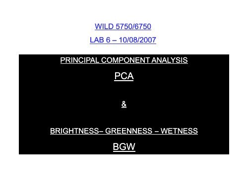
WILD 5750/6750<br />
LAB 6 – 10/08/2007<br />
PRINCIPAL COMPONENT ANALYSIS<br />
PCA<br />
&<br />
BRIGHTNESS– GREENNESS – WETNESS<br />
BGW
Lecture review…<br />
Transformation of a set of correlated<br />
variables (i.e. b<strong>and</strong>s) into a new set of<br />
uncorrelated variables (PC).<br />
Rotation of the original axes to new<br />
orientations ti that t are orthogonal to<br />
each other with little or no correlation<br />
between variables<br />
For remote sensing studies = predominantly exploratory in nature<br />
Used to help in the extraction of features <strong>and</strong> to reduce dimensionality of data<br />
After Lilles<strong>and</strong> <strong>and</strong> Keifer, 1994 – Lecture materials
Imagine… inputs + process<br />
Interpreter Spectral Enhancement Principal Components<br />
Save disk space: Stretch (0 – 255) but no further math post-<br />
processing<br />
Obtain Eigenvectors matrix + Eigenvalues table
Imagine… inputs + process<br />
Interpreter t Spectral Enhancement Pi Principal i lComponents<br />
Keep the<br />
output t as<br />
Float<br />
Eigenvectors<br />
matrix<br />
Eigenvalues table<br />
Number of<br />
PC to keep:<br />
1= Not<br />
useful<br />
6: Too<br />
many
Imagine… results<br />
Eigenvalues table:<br />
% _ Variance<br />
eigenvalueλ<br />
px100<br />
= 6<br />
∑<br />
p=1<br />
eigenvalueλ λ p<br />
How much variability was<br />
captured in each new PC<br />
Eigenvectors matrix:<br />
How each new PC b<strong>and</strong> is<br />
obtained<br />
Multiply each original TM<br />
b<strong>and</strong> by the eigenvectors<br />
Sum the products to<br />
Sum the products to<br />
obtain the new Digital<br />
numbers DN
Imagine… results<br />
ViewerFile<br />
FileOpen<br />
OpenMulti layer arrangement<br />
1 2 3<br />
4 5 6<br />
1: > Variance // 6: < Variance ~ Noise
Imagine… results<br />
Factor loadings = what type of component (i.e. visible, infrared) is it<br />
R<br />
kp<br />
=<br />
a<br />
kp<br />
x<br />
S<br />
k<br />
λ<br />
p<br />
Rkp: Factor loading<br />
akp:Eigenvectorp for b<strong>and</strong> k <strong>and</strong> component p<br />
λp: Eigenvalue for the pth component<br />
Sk: St<strong>and</strong>ard deviation for b<strong>and</strong> k
Assignment – Part A<br />
•Brief description of PCA as a general statistical tool <strong>and</strong> its use for image processing –<br />
use your book, lecture materials <strong>and</strong> Internet.<br />
•Perform the PCA analysis for an image of your choice (if you do not have one of your own,<br />
then use a small subset of the Rich county image)<br />
•http://leupold.gis.usu.edu/~alex/WILD6750_lab_6/PCA_image_Calcs/<br />
•Create snapshots of the input file, the output file, <strong>and</strong> individual b<strong>and</strong>s.<br />
•Report the table for the Eigenvalues <strong>and</strong> the matrix of Eigenvectors<br />
•Determine the amount (%) of information contained in each b<strong>and</strong> using the<br />
Eigenvalues<br />
•Interpret each output b<strong>and</strong> <strong>and</strong> describe what the information contained in each<br />
consists of (visual interpretation & factor loadings).<br />
•http://leupold.gis.usu.edu/~alex/WILD6750_lab_6/PCA_image_Calcs/<br />
•Of what use - if any - are the last set of components<br />
Jensen, 2005 -
Lecture review…<br />
<strong>Brightness</strong> defined in the direction of soil<br />
reflectance variation. Obtained from a weighted<br />
sum of all b<strong>and</strong>s. i.e. urbanized <strong>and</strong> bare soil<br />
areas are evident in this image.<br />
Greenness defined in the direction of<br />
vegetation reflectance variation. Obtained from<br />
the contrast of the visible b<strong>and</strong>s (high absorption)<br />
with the infrared b<strong>and</strong>s (high reflectance). i.e. the<br />
greater the biomass, the brighter the pixel value<br />
in this image.<br />
Greenness<br />
Water<br />
Healthy – dense<br />
vegetation<br />
Clear Turbid<br />
<strong>Brightness</strong><br />
Concrete<br />
Bare soil<br />
Wetness information concerning the moisture<br />
status of the environment (soil & plant moisture).<br />
Obtained from the contrast of the sum of visible<br />
<strong>and</strong> near-infrared with the sum of longer-infrared<br />
b<strong>and</strong>s. i.e. water bodies are very bright – greater<br />
the moisture content = brighter response.<br />
Third<br />
Water<br />
Clear Turbid<br />
Wet soil<br />
<strong>Brightness</strong><br />
Concrete –<br />
Bare soil<br />
Dry soil<br />
Jensen - 2005
Imagine… input + process<br />
Float<br />
1 st three channels are:<br />
(1) <strong>Brightness</strong>, (2)<br />
Greenness, <strong>and</strong> (3)<br />
Wetness<br />
Huang <strong>and</strong> others, 2002<br />
At-sensor reflectance coefficients
Imagine… input + process<br />
We need a model will the following components:<br />
a) Input image: L<strong>and</strong>sat TM B<strong>and</strong>s 1, 2, 3, 4, 5, <strong>and</strong> 7<br />
b) Transformation coefficients i for each b<strong>and</strong> <strong>and</strong> for each<br />
main axis B, G, W<br />
c) A linear combination function<br />
d) Output image (float)
Imagine… results<br />
ViewerFileOpenThree layer arrangement<br />
B<br />
G<br />
W
Assignment – Part B<br />
• We have 3 images for 3 different periods for the Camp Williams – Utah Lake area<br />
(CWUL_Aug99.img, CWUL_Oct99.img, <strong>and</strong> CWUL_May00). Obtain BGW indices<br />
for each of these images using the previously defined model <strong>and</strong> coefficients.<br />
• Provide snapshots of the 3 results similar to the depiction in the previous slide.<br />
Please label appropriately for each temporal scenario.<br />
• By visually comparing the indices, what major changes do you see i.e. brightness differences<br />
among temporal scenarios. What do you think is the cause for such changes - If any –<br />
-----------------------------------------------------------------------------------------------------------------------------------<br />
• We also have as ancillary data an image (GAP-CWUL.img) which contains l<strong>and</strong> cover<br />
categories from the SWRGAP project. This image can be used - Hopefully !! – to see the<br />
rationale of our 3 Greenness indices across time.<br />
(a) Briefly, how would you derive simple inferences Hint! – Think about seasonal precipitation<br />
<strong>and</strong> phenology patterns<br />
(b) Choose two l<strong>and</strong> cover categories (of your choice), <strong>and</strong> record 5 values for each l<strong>and</strong> cover<br />
category <strong>and</strong> for each temporal scenario (Greenness indices only). Prepare a table with these<br />
values <strong>and</strong> a simple graph <strong>and</strong> include them in your report. Does this help you for answering (a)<br />
(c) Briefly, mention 3 examples for which you would use BGW indices<br />
Have fun!
a) In a viewer, load the L<strong>and</strong> cover image<br />
b) Select two l<strong>and</strong> cover categories – your choice -<br />
c) For each category, determine the location (X, Y coordinates) for 5 points of your choice – try to<br />
select these points so that they are spread over the image but within the l<strong>and</strong> cover category that<br />
you are assessing<br />
d) Write down those coordinates<br />
e) In a new viewer, load one of the BGW images you just derived<br />
f) Extract the pixel information – not the LUT value! – for each one of the 5 points for the<br />
GREENNESS channel<br />
g) Repeat (e) <strong>and</strong> (f) for the other two BGW images<br />
h) Record your values in a table / prepare a simple graph <strong>and</strong> annotate your observations
Suggested readings…<br />
• Your book! Jensen – 2005 – Image enhancement – Vegetation transformation indices Chapter 8<br />
• I will send digital copies of these by email <br />
I will send digital copies of these by email <br />
• Christ & Cicone – 1984 – A physically-based transformation of Thematic Mapper Data – The TM<br />
Tasseled Cap<br />
• Christ & Kauth – 1986 – The Tasseled Cap De-Mystified<br />
• Huang <strong>and</strong> others – 2002 - Derivation of a Tasseled Cap transformation based on L<strong>and</strong>sat 7<br />
at-satellite reflectance