Molecular Dynamics Chapter 2. Molecular Dynamics in Various ...

Molecular Dynamics
Chapter 2. Molecular Dynamics in Various Ensembles
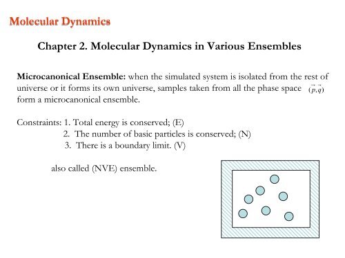
Microcanonical Ensemble: when the simulated system is isolated from the rest of
universe or it forms its own universe, samples taken from all the phase space ( p,
q)
form a microcanonical ensemble.
Constraints: 1. Total energy is conserved; (E)
2. The number of basic particles is conserved; (N)
3. There is a boundary limit. (V)
also called (NVE) ensemble.

Molecular Dynamics Chapter 2.1
Basic Thermodynamics
Equilibrium: when samples can be meaningfully used for state-function
(thermodynamic property) measurements, system is in equilibrium.
1. It is a relative concept, dependent on overall sampling length.
2. It is a concept conditioned by ergodic requirements.

Molecular Dynamics Chapter 2.1
Basic Thermodynamics
Second law of thermodynamics: maximum entropy theorem
During the course of system’s approaching the equilibrium state, entropy is
maximized when the total energy is conserved. (NVE)
Alternative: minimum energy theorem
During the course of system’s approaching the equilibrium state,
energy is minimized when the entropy is conserved (NVS).
Entropy: a measure of system diversity (disorder).
dQ
dS = ( )
T
resersible
dE
dV
= dQ + dW
= 0 , dW = 0
1 / = (
dS
dE
)
T
N , V

Molecular Dynamics Chapter 2.1
Basic Thermodynamics – Statistical Mechanics
1 / =
(
dS
dE
)
T
N , V
NkT
= ∑
2
m i
v i
For a large subset of a huge system, in the equilibrium state,
Total E= E 1 +E 2 under mean field condition
If Ω( E,
V , N ) represents the occurrence probability (or degeneracy)
∑
Γ
Ω ( E,
V , N)
= δ ( H ( Γ)
− E)
s = k lnΩ

Molecular Dynamics Chapter 2.1
Basic Thermodynamics – Statistical Mechanics
1 / =
(
dS
dE
)
T
N , V
NkT
= ∑
2
m i
v i
For a large subset of a huge system, in the equilibrium state,
Total E= E 1 +E 2 under mean field condition
s
= k ln
Ω
⎛ ∂k
ln Ω(
E , E − E
⎜
⎝ ∂E1
) ⎞
⎟
⎠
1 1
=
N , V , E
0
⎛ ∂k
ln Ω(
E1 , V , N)
⎜
⎝ ∂E1
⎞
⎟
⎠
N , V , E
= β
β = 1/(
kT )

Molecular Dynamics Chapter 2.1
Basic Statistical Mechanics
Simple example: (NVE)
Two state potential energy function: E = (E 0 , E 1 ) for two recognizable particles
Total energy E 0 + E 1
E 1
E 1
Ω = 2
E 0
E 0
s
=
k
ln 2
k
= 1.38E
−
23

Molecular Dynamics Chapter 2.1
Basic Statistical Mechanics
Simple example: (NVE)
Two state potential energy function: E = (0, E 0 , E 1 , E 0 + E 1 ) for two recognizable
particles. Total energy E 0 + E 1
E 0 + E 1
E 1
4
E 0
0
Ω =
s
=
k
ln 4
k
= 1.38E
−
23

Molecular Dynamics Chapter 2.1
Microcanonical Ensemble
Microcanonical Ensemble in MD simulation:
1. The occurrence probability is independent of subset of energies.
2. Ensemble property is dependent on the maximum entropy.
3. Easy to implement.
4. Difficult to control macroscopic condition.
5. It can be used as thermo reservoir for canonical ensemble simulations.

Molecular Dynamics Chapter 2.2
Canonical Ensemble
Canonical Ensemble: when the simulated system is embedded in an infinite
heat bath, but does not have particle exchange with this bath, it forms a
canonical ensemble.
Constraints: 1. System temperature is conserved (not absolutely constant); (T)
2. The number of basic particles is conserved; (N)
3. There is a boundary limit (V); or there is a constant pressure (P)
also called (NVT) ensemble or (NPT) ensemble.

Molecular Dynamics Chapter 2.1
Canonical Ensemble
Canonical ensemble can be considered as a sub-microcanonical ensemble, where
particle collisions occur on the “boundary”.
In practice, the temperature buffer region can be flexibly designed and its
boundary with the simulated region can also be flexibly designed.
Centers of canonical ensemble algorithm developments

Molecular Dynamics Chapter 2.1
Canonical Ensemble
Canonical ensemble can be derived from microcanonical ensemble, too.
EB
E
A
E = E A
+ EB
For a given system energy E A , reservoir probability determines its probability.
Ω(
E − E ) A
In micro-canonical ensemble, higher energy has larger probability. Why
So lower system energy should have larger probability. Why

Molecular Dynamics Chapter 2.1
Canonical Ensemble
EB
E
A
E = E A
+ EB
For a given system energy E A , reservoir probability determines its probability.
Because simulated system is much smaller than the buffer portion,
Taylor expansion:
∂ ln Ω(
E)
ln Ω(
E − E
A
) = ln Ω(
E)
− E
A
= ln Ω(
E)
− E
A
/ kT
∂E
Probability for the system with energy E A :
P(
E
A
)
=
exp( −E
∑
i
A
exp( −E
/
i
kT )
/ kT )

Molecular Dynamics Chapter 2.1
Canonical Ensemble
P(
E
A
)
=
exp( −E
∑
i
A
exp( −E
/
i
kT )
/ kT )
We should learn from this derivation on canonical ensemble algorithm design:
1. The thermal reservoir is essential, because it governs the Boltzmann
distribution.
2. The thermal volume of the thermal reservoir should be large enough to
reflect the Taylor expension.

Molecular Dynamics Chapter 1.1
Temperature in Canonical Ensemble
3
E K
=
2
NkT
Canonical ensemble is not absolutely constant-temperature or
isokinetic ensemble.
Maxwell-Boltzmann distribution:
ρ(|
p
|)
=
⎛
⎜
⎝
β
2πm
⎞
⎟
⎠
3 / 2
exp
[ | | /(2 )]
2
− β p m

Molecular Dynamics Chapter 1.1
Thermal Reservoir Algorithm Design
• Reservoir can be flexible, represented by other natures of particle, force,
or interactions.
2. Coupling boundary can also be flexible, not restrained by the spatial boundary.
3. Computation overhead should be small.
4. Preserve canonical ensemble: temperature
and Maxwell-Boltzmann distribution.

Molecular Dynamics Chapter 1.1
The Simplest Algorithm: Velocity Re-scaling
ΔT
=
N
1 2 i
λ
i
2
∑
i=
1
3
m
(
Nk
v
B
)
2
−
1
2
N
∑
i=
1
2
3
m v
i
Nk
2
i
B
ΔT
=
( λ
2 −1)
T ( t)
λ =
T new
/ T ( t)
T
=
new
T t arg et

Molecular Dynamics Chapter 1.1
The Simplest Algorithm: Velocity Re-scaling
1. Not real canonical ensemble, although it is close.
2. Maxwell-Boltzmann distribution can not be guaranteed. Scaling frequency is not
robust (ad hoc).
3. Propagation stability can be destroyed.
4. How to make judgments during the simulations
kinetic energy and potential energy exchange.

Molecular Dynamics Chapter 1.1
Berendsen Thermostat
Velocity Re-scaling scheme has absolute target temperature every time-step.
To generate a temperature fluctuation, the difference between the target temperature
and the instantaneous temperature can be used to drive the temperature change
dT ( t)
dt
= 1
( T
τ
bath −
T ( t))
The temperature change between successive time steps is:
ΔT
=
δt
( Tbath − T ( t))
τ

Molecular Dynamics Chapter 1.1
Berendsen Thermostat
In practice, we need to perform a temperature dependent velocity rescaling:
2
λ
δt
⎛ Tbath
⎞
= 1+
⎜ −1⎟
τ ⎝ T ( t)
⎠
When the coupling parameter is equal to the time step, berendsen thermostat is
equivalent to the velocity rescaling method.
For large uniform systems, scaling ratio δt/τ = 0.0025 can produce a pseudo
Maxwell-Boltzmann Distribution.

Molecular Dynamics Chapter 1.1
Local Temperature Trapping
The temperature fluctuation is important for the
trapped kinetic energy to be released.
When a large scaling ratio is applied, the
temperature fluctuation will be prohibited.
When a small scaling ratio is applied, the
temperature averaging can not be easily
guaranteed.
Hot spot
Intrinsic problem: thermo-diffusivity is low.

Molecular Dynamics Chapter 1.1
Stochastic Collision method:
Anderson Thermostat
The velocities of randomly selected particles are randomly reset, based on
Maxwell-Boltzmann distribution.
Random selection: if random number [0, 1] > νdt,
ν is stochastic collision frequency
dt is the time step.
the corresponding particle is selected.
Random Reset:
distribution.
Gaussian(velocity) based on Maxwell-Boltzmann

Molecular Dynamics Chapter 1.1
Integration: Velocity Verlet Algorithm
r
v
F
t-Δt t t+Δt
Given current position,
velocity, and force

Molecular Dynamics Chapter 1.1
Integration: Velocity Verlet Algorithm
r
v
F
t-Δt t t+Δt
Compute new position

Molecular Dynamics Chapter 1.1
Integration: Velocity Verlet Algorithm
r
v
F
t-Δt t t+Δt
Compute velocity at half step

Molecular Dynamics Chapter 1.1
Integration: Velocity Verlet Algorithm
r
v
F
t-Δt t t+Δt
Compute force at new position

Molecular Dynamics Chapter 1.1
Integration: Velocity Verlet Algorithm
r
v
F
t-Δt t t+Δt
Compute velocity at full step
At this step, some particles’ velocities will be reset based on
the Anderson formulation.

Molecular Dynamics Chapter 1.1
Integration: Velocity Verlet Algorithm
r
v
F
t-2Δt t-Δt t t+Δt
Advance to next time step,
repeat

Molecular Dynamics Chapter 1.1
Stochastic Collision method:
Anderson Thermostat
The Anderson process is equivalent to the Monte Carlo move.
This process becomes a Markov process (no memory). And the
canonical distribution (Boltzmann distribution) can be guaranteed.
Question: Can we provide random input from Force rather than
Velocity If so, which integrator is ideal What is the advantage and
What is the disadvantage

Molecular Dynamics Chapter 1.1
Stochastic Collision method:
Anderson Thermostat
Frequency influence on the phase space exploration:
If frequency is too high, collision will dominate and inhibit an efficient
exploration of the phase space to meet the ergodic requirement.
If frequency is too low, the canonical distribution will be formed slowly
to meet the canonical requirement.
Suggested collision rate:
ρ
Cλ
T
1/ 3 2 / 3
N

Molecular Dynamics Chapter 1.1
Extended Hamiltonian Approach
H
1 2
d s r
H M k s s
2
extended
=
o
+
r
+
r r − +
2
dt
1
2
U
bias
( s,
t)
Any targeted property: temperature, pressure, energy difference,
geometry, … can be coupled to the original Hamiltonian to achieve
the desired distributions.
It is equivalent to the biased Monte Carlo.

Molecular Dynamics Chapter 1.1
Nose-Hoover Thermostat
H
extended
N
= U
o
+ ∑
i=
1
p
2
i
2m s
i
2
r
+
1
2
M
r
ds
dt
r
2
+
L
ln sr
β
1. S r has to be greater than 1. (Lagrangian multiplier)
2. S r plays a role in rescaling the time-step.
3. So, the real time step fluctuates.
4. The Q is equivalent to the Q of the canonical ensemble.

Molecular Dynamics Chapter 2.2
Grand Canonical Ensemble
Grand Canonical Ensemble: when the simulated system is embedded in an
infinite heat bath, and can exchange particle with the infinite particle reservoir, it
forms a grand canonical ensemble.
Constraints: 1. System temperature is conserved (not absolutely constant); (T)
2. The chemical potential of the particle reservoir is constant (μ)
3. There is a boundary limit (V); or there is a constant pressure (P)
also called (GVT) ensemble or (GPT) ensemble.

Molecular Dynamics Chapter 2.1
Grand Canonical Ensemble
Canonical ensemble can be considered as a sub-microcanonical ensemble, where
particle collisions and exchanges occur on the “boundary”.
In practice, the reservoir buffer region can be flexibly designed and its
boundary with the simulated region can also be flexibly designed.
Centers of grand canonical ensemble algorithm developments

Molecular Dynamics Chapter 2.1
Canonical Ensemble
P(
E
A
)
=
exp( −E
∑
i
A
exp( −E
/
i
kT )
/ kT )
How to write Grand Canonical Ensemble partition function:
P
∞
∑
N = 0
=
( N!)
−1
V
N
z
Q
N
∫
μVT
dr
exp( −βE)
z
=
( h
2
exp( βμ )
/ 2πmk
T )
B
3/ 2

Molecular Dynamics Chapter 2.1
How to Realize Grand Canonical Ensemble in Monte Carlo
1. Internal Displacements
ρ
accp
=
min( 1,exp( −βE))
2. Insertion and removal
ρ
ρ
accp
accp
=
−
min( 1,exp( −β
( En
1
+ u − En))
=
+
min( 1,exp( −β
( En
1
− u − En))

Molecular Dynamics Chapter 2.1
Hybrid Monte Carlo for Grand Canonical Ensemble
1. Internal Displacements Canonical ensemble Molecular Dynamics
2. Insertion and removal ρaccp
= min( 1,exp( −β
( En−
1
+ u − En))
ρ
accp
=
+
min( 1,exp( −β
( En
1
− u − En))

Molecular Dynamics Chapter 2.1
Extended Hamiltonian to Realize Grand Canonical Ensemble

Molecular Dynamics Chapter 2.1
Extended Hamiltonian to Realize Grand Canonical Ensemble
One particle scheme:
H
extended
1 dsr
= H
o
( n −1)
+ M
r
+ sr
( U
o
− μ ) + μ
2 dt
0≤ S r
≤1
2

Molecular Dynamics Chapter 2.1
Extended Hamiltonian to Realize Grand Canonical Ensemble
One particle scheme:
H
extended
1 dsr
= H
o
( n −1)
+ M
r
+ sr
( U
o
− μ ) + μ
2 dt
0≤ S r
≤1
2
Drawbacks: 1. Particle number fluctuation magnitude can be larger
than 1.
2. When Sr = 0, it can take long simulation time for the ghost
particle to locate a position again. Why
Interaction Singularity.

Molecular Dynamics Chapter 2.1
Extended Hamiltonian to Realize Grand Canonical Ensemble
One particle scheme:
H
extended
1 dsr
= H
o
( n −1)
+ M
r
+ sr
( U
o
− μ ) + μ
2 dt
2
0≤ S r
≤1
How to solve the interaction singularity, when S r
= 0
Two General Strategies: 1. Make the switching S r
(U o
-μ) nonlinear.
2. Adiabatic switching method

Molecular Dynamics Chapter 2.1
Extended Hamiltonian to Realize Grand Canonical Ensemble
One particle scheme:
H
extended
1 dsr
= H
o
( n −1)
+ M
r
+ srU
o
− srμ + μ
2 dt
2
0≤ S r
≤1
Nonlinear switching S r
U o
Original Lennard-Jones interaction:
Nonlinear Switching (Softcore potential):
⎡ A B
ε ⎢ 12
− 6
⎣r
r
⎤
⎥
⎦
s
r
⎧ ⎡
⎨ε
⎢
⎩ ⎣
A
+ σ (1 −
−
B
+ σ (1 −
2
6 2
( r sr
)) ( r sr
))
3
⎤⎫
⎥⎬
⎦⎭

Molecular Dynamics Chapter 2.1
Extended Hamiltonian to Realize Grand Canonical Ensemble
⎧ ⎡
⎨ε
⎢
⎩ ⎣
A
B
−
2
6 2
( r + σ (1 − sr
)) ( r + σ (1 − sr
))
3
⎤⎫
⎥⎬
⎦⎭
Another Advantage:

Molecular Dynamics Chapter 2.1
Extended Hamiltonian to Realize Grand Canonical Ensemble
Adiabatic switching method: Extended Hamiltonian Hybrid Monte Carlo
H
extended
1 dsr
= H
o
( n −1)
+ M
r
+ sr
( U
o
− μ ) + μ
2 dt
2
1. When Sr = 0 or 1, at a pre-set time interval N*τ, fixing the position
of the ghost particle.
2. Adiabatically switch Sr from 0 to 1 or switch Sr from 1 to 0, the
energy change will be E − or E −
n−1
E n
n+1
E n
ρ
ρ
accp
accp
=
−
min( 1,exp( −β
( En
1
+ u − En))
=
+
min( 1,exp( −β
( En
1
− u − En))