
You also want an ePaper? Increase the reach of your titles
YUMPU automatically turns print PDFs into web optimized ePapers that Google loves.
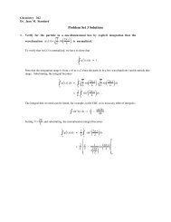
4<br />
3. Continued<br />
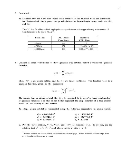
d). Estimate how the CPU time would scale relative to the minimal basis set calculation<br />
for Hartree-Fock single point energy calculations on benzaldehyde using basis sets (b)<br />
and (c).<br />
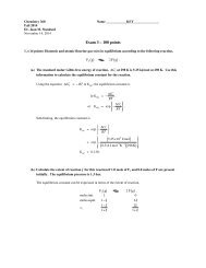
The CPU time for a Hartree-Fock single point energy calculation scales approximately as the number of<br />
basis functions to the power 3.5, K 3.5 .<br />
Basis <strong>Set</strong><br />
No. Basis<br />
Functions<br />
Relative<br />
CPU Time<br />
minimal 46 1<br />
6-31G(d) 124 (124/46) 3.5 = 32<br />
6-311G(d,p) 180 (180/46) 3.5 = 119<br />
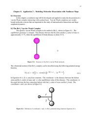
4. Consider a linear combination of three gaussian type orbitals, called a contracted gaussian<br />
function,<br />
f (r) =<br />
3<br />
∑ c i G i (r) ,<br />
i=1<br />
where f (r) is an atomic orbital, and the c i s are linear coefficient.<br />
gaussian function, given by € the expression<br />
The function<br />
G i (r) is a<br />
€<br />
€<br />
G i (r) =<br />
⎛⎛<br />
⎜⎜<br />
⎝⎝<br />
2α i<br />
π<br />
3/ 4<br />
⎞⎞<br />
⎟⎟ e −α i r 2 .<br />
⎠⎠<br />
€<br />
The reason that an atomic orbital like f (r) is expressed in terms of a linear combination<br />
of gaussian functions is so € that it can better represent the cusp behavior of a true atomic<br />
orbital in the vicinity of the nucleus.<br />
€<br />
An s-type atomic orbital is represented using the following parameters (in atomic units):<br />
d 1 = 4.44635×10 –1 α 1 = 1.09818×10 –1<br />
d 2 = 5.35328×10 –1 α 2 = 4.05771×10 –1<br />
d 3 = 1.54329×10 –1 α 3 = 2.22766<br />
a.) Plot the three orbitals, G 1 (r) , G 2 (r) , and G 3 (r), as functions of x.<br />
relation that r 2 = x 2 + y 2 + z 2 , and plot a cut for x with y = z = 0.<br />
To do this, use the<br />
The three orbitals are € shown € plotted individually € on the next page. Notice that the functions range from<br />
quite broad € to fairly narrow in extent.<br />
€