Problem Set 9 Solutions

More documents

Recommendations

Info

4 3. Continued d). Estimate how the CPU time would scale relative to the minimal basis set calculation for Hartree-Fock single point energy calculations on benzaldehyde using basis sets (b) and (c). The CPU time for a Hartree-Fock single point energy calculation scales approximately as the number of basis functions to the power 3.5, K 3.5 . Basis <strong>Set</strong> No. Basis Functions Relative CPU Time minimal 46 1 6-31G(d) 124 (124/46) 3.5 = 32 6-311G(d,p) 180 (180/46) 3.5 = 119 4. Consider a linear combination of three gaussian type orbitals, called a contracted gaussian function, f (r) = 3 ∑ c i G i (r) , i=1 where f (r) is an atomic orbital, and the c i s are linear coefficient. gaussian function, given by € the expression The function G i (r) is a € € G i (r) = ⎛⎛ ⎜⎜ ⎝⎝ 2α i π 3/ 4 ⎞⎞ ⎟⎟ e −α i r 2 . ⎠⎠ € The reason that an atomic orbital like f (r) is expressed in terms of a linear combination of gaussian functions is so € that it can better represent the cusp behavior of a true atomic orbital in the vicinity of the nucleus. € An s-type atomic orbital is represented using the following parameters (in atomic units): d 1 = 4.44635×10 –1 α 1 = 1.09818×10 –1 d 2 = 5.35328×10 –1 α 2 = 4.05771×10 –1 d 3 = 1.54329×10 –1 α 3 = 2.22766 a.) Plot the three orbitals, G 1 (r) , G 2 (r) , and G 3 (r), as functions of x. relation that r 2 = x 2 + y 2 + z 2 , and plot a cut for x with y = z = 0. To do this, use the The three orbitals are € shown € plotted individually € on the next page. Notice that the functions range from quite broad € to fairly narrow in extent. €
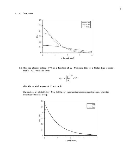
5 4. a.) Continued 0.6 0.5 G1(x) G2(x) G3(x) 0.4 G(x) 0.3 0.2 0.1 0 0 1 2 3 4 x (angstroms) b.) Plot the atomic orbital f (r) as a function of x. orbital s(r) with the form Compare this to a Slater type atomic € € s(r) = ζ 3 1/ 2 ⎛⎛ ⎞⎞ ⎜⎜ ⎜⎜ ⎟⎟ ⎝⎝ π ⎟⎟ e −ζ r , ⎠⎠ with the orbital exponent ζ set to 1. € The functions are plotted below. Note that the only significant difference is near the origin, where the Slater type orbital has € a cusp. 0.6 0.5 s(x) f(x) 0.4 s(x), f(x) 0.3 0.2 0.1 0 0 1 2 3 4 x (angstroms)
Page 1 and 2: Chemistry 460 Dr. Jean M. Standard
Page 3: 3 3. Suppose you want to carry out
Page 7 and 8: 7 5 b.) continued The third MO (whi
Page 9 and 10: 9 6. A Hartree-Fock SCF calculation

Problem Set 9 Solutions

Create successful ePaper yourself

Delete template?

Save as template?