Distributed Reactive Collision Avoidance - University of Washington
Distributed Reactive Collision Avoidance - University of Washington
Distributed Reactive Collision Avoidance - University of Washington

You also want an ePaper? Increase the reach of your titles
YUMPU automatically turns print PDFs into web optimized ePapers that Google loves.
<strong>Distributed</strong> <strong>Reactive</strong> <strong>Collision</strong> <strong>Avoidance</strong><br />
Emmett Lalish<br />
A dissertation submitted in partial fulfillment<br />
<strong>of</strong> the requirements for the degree <strong>of</strong><br />
Doctor <strong>of</strong> Philosophy<br />
<strong>University</strong> <strong>of</strong> <strong>Washington</strong><br />
2009<br />
Program Authorized to Offer Degree: Aeronautics and Astronautics
<strong>University</strong> <strong>of</strong> <strong>Washington</strong><br />
Graduate School<br />
This is to certify that I have examined this copy <strong>of</strong> a doctoral dissertation by<br />
Emmett Lalish<br />
and have found that it is complete and satisfactory in all respects,<br />
and that any and all revisions required by the final<br />
examining committee have been made.<br />
Chair <strong>of</strong> the Supervisory Committee:<br />
Kristi A. Morgansen<br />
Reading Committee:<br />
Kristi A. Morgansen<br />
Mehran Mesbahi<br />
Juris Vagners<br />
Date:
In presenting this dissertation in partial fulfillment <strong>of</strong> the requirements for the doctoral<br />
degree at the <strong>University</strong> <strong>of</strong> <strong>Washington</strong>, I agree that the Library shall make its copies<br />
freely available for inspection. I further agree that extensive copying <strong>of</strong> this dissertation<br />
is allowable only for scholarly purposes, consistent with “fair use” as prescribed in the U.S.<br />
Copyright Law. Requests for copying or reproduction <strong>of</strong> this dissertation may be referred<br />
to Proquest Information and Learning, 300 North Zeeb Road, Ann Arbor, MI 48106-1346,<br />
1-800-521-0600, to whom the author has granted “the right to reproduce and sell (a) copies<br />
<strong>of</strong> the manuscript in micr<strong>of</strong>orm and/or (b) printed copies <strong>of</strong> the manuscript made from<br />
micr<strong>of</strong>orm.”<br />
Signature<br />
Date
<strong>University</strong> <strong>of</strong> <strong>Washington</strong><br />
Abstract<br />
<strong>Distributed</strong> <strong>Reactive</strong> <strong>Collision</strong> <strong>Avoidance</strong><br />
Emmett Lalish<br />
Chair <strong>of</strong> the Supervisory Committee:<br />
Pr<strong>of</strong>essor Kristi A. Morgansen<br />
Aeronautics and Astronautics<br />
<strong>Collision</strong> avoidance is an important aspect <strong>of</strong> multivehicle coordination because it prevents<br />
vehicles from disrupting or destroying each other. The work contained in this dissertation<br />
concerns a novel approach to the n-vehicle collision avoidance problem. The vehicle model<br />
used here allows for three-dimensional movement and represents a wide range <strong>of</strong> vehicles.<br />
The algorithm works in conjunction with any desired controller to guarantee all vehicles<br />
remain free <strong>of</strong> collisions while attempting to follow their desired control. This algorithm<br />
is reactive and distributed, making it well-suited for real-time applications, and explicitly<br />
accounts for actuation limits. A robustness analysis is presented which provides a means to<br />
account for delays and unmodeled dynamics. Robustness to an adversarial vehicle is also<br />
presented.
TABLE OF CONTENTS<br />
Page<br />
List <strong>of</strong> Figures . . . . . . . . . . . . . . . . . . . . . . . . . . . . . . . . . . . . . .<br />
iii<br />
List <strong>of</strong> Tables . . . . . . . . . . . . . . . . . . . . . . . . . . . . . . . . . . . . . . iv<br />
Chapter 1: Introduction to <strong>Collision</strong> <strong>Avoidance</strong> . . . . . . . . . . . . . . . . . . 1<br />
1.1 Definitions <strong>of</strong> Terms . . . . . . . . . . . . . . . . . . . . . . . . . . . . . 3<br />
1.2 Literature Review . . . . . . . . . . . . . . . . . . . . . . . . . . . . . . . 6<br />
1.3 Introduction to DRCA . . . . . . . . . . . . . . . . . . . . . . . . . . . . 11<br />
Chapter 2: Problem Statement . . . . . . . . . . . . . . . . . . . . . . . . . . . 13<br />
Chapter 3: Conflicts and <strong>Collision</strong>s . . . . . . . . . . . . . . . . . . . . . . . . 17<br />
Chapter 4: DRCA Algorithm . . . . . . . . . . . . . . . . . . . . . . . . . . . . 20<br />
4.1 Deconfliction Maneuvers . . . . . . . . . . . . . . . . . . . . . . . . . . . 23<br />
4.1.1 Constant-Speed Maneuver . . . . . . . . . . . . . . . . . . . . . . 25<br />
4.1.2 Variable-Speed Maneuver . . . . . . . . . . . . . . . . . . . . . . 29<br />
4.1.3 Heuristic Performance . . . . . . . . . . . . . . . . . . . . . . . . 34<br />
4.2 Deconfliction Maintenance . . . . . . . . . . . . . . . . . . . . . . . . . . 36<br />
4.2.1 Control Law . . . . . . . . . . . . . . . . . . . . . . . . . . . . . 36<br />
4.2.2 Guarantee . . . . . . . . . . . . . . . . . . . . . . . . . . . . . . . 39<br />
4.2.3 Priority . . . . . . . . . . . . . . . . . . . . . . . . . . . . . . . . 43<br />
4.2.4 Behavior . . . . . . . . . . . . . . . . . . . . . . . . . . . . . . . 44<br />
4.2.5 Liveness . . . . . . . . . . . . . . . . . . . . . . . . . . . . . . . 45<br />
Chapter 5: Robustness Analysis . . . . . . . . . . . . . . . . . . . . . . . . . . 48<br />
5.1 Robust Stability . . . . . . . . . . . . . . . . . . . . . . . . . . . . . . . . 48<br />
5.2 Robust <strong>Avoidance</strong> . . . . . . . . . . . . . . . . . . . . . . . . . . . . . . . 51<br />
i
Chapter 6: Performance . . . . . . . . . . . . . . . . . . . . . . . . . . . . . . 54<br />
6.1 Variable Speed . . . . . . . . . . . . . . . . . . . . . . . . . . . . . . . . 54<br />
6.2 Preferential Routing . . . . . . . . . . . . . . . . . . . . . . . . . . . . . . 56<br />
6.3 Three-dimensional <strong>Avoidance</strong> . . . . . . . . . . . . . . . . . . . . . . . . 58<br />
6.4 Heuristic Performance . . . . . . . . . . . . . . . . . . . . . . . . . . . . 59<br />
6.5 Computational Scaling . . . . . . . . . . . . . . . . . . . . . . . . . . . . 62<br />
6.6 Formations . . . . . . . . . . . . . . . . . . . . . . . . . . . . . . . . . . 63<br />
6.7 Comparison to an SGT Algorithm . . . . . . . . . . . . . . . . . . . . . . 65<br />
Chapter 7: Conclusion . . . . . . . . . . . . . . . . . . . . . . . . . . . . . . . 69<br />
7.1 Future Work . . . . . . . . . . . . . . . . . . . . . . . . . . . . . . . . . . 70<br />
Bibliography . . . . . . . . . . . . . . . . . . . . . . . . . . . . . . . . . . . . . . 72<br />
ii
LIST OF FIGURES<br />
Figure Number<br />
Page<br />
1.1 Air traffic control. . . . . . . . . . . . . . . . . . . . . . . . . . . . . . . . 2<br />
3.1 Geometric definition <strong>of</strong> the collision cone. . . . . . . . . . . . . . . . . . . 18<br />
4.1 Flow chart <strong>of</strong> the DRCA algorithm. . . . . . . . . . . . . . . . . . . . . . 21<br />
4.2 Example optimization <strong>of</strong> a constant-speed maneuver. . . . . . . . . . . . . 25<br />
4.3 Example <strong>of</strong> an infeasible constant-speed maneuver problem. . . . . . . . . 30<br />
4.4 Example optimization <strong>of</strong> a variable-speed maneuver. . . . . . . . . . . . . 31<br />
4.5 Example <strong>of</strong> an infeasible variable-speed maneuver problem. . . . . . . . . 34<br />
4.6 Block diagram <strong>of</strong> the deconfliction maintenance controller. . . . . . . . . . 36<br />
4.7 Geometry <strong>of</strong> the conflict measures p t and p n . . . . . . . . . . . . . . . . . 37<br />
4.8 Example <strong>of</strong> the control function, F . . . . . . . . . . . . . . . . . . . . . . 39<br />
5.1 Geometry <strong>of</strong> worst case adversary . . . . . . . . . . . . . . . . . . . . . . 53<br />
6.1 Five vehicle simulation. . . . . . . . . . . . . . . . . . . . . . . . . . . . . 55<br />
6.2 Excess separation <strong>of</strong> vehicles in Fig. 6.1. . . . . . . . . . . . . . . . . . . . 55<br />
6.3 Preferential routing comparison for three vehicles. . . . . . . . . . . . . . . 57<br />
6.4 Three-dimensional collision avoidance. . . . . . . . . . . . . . . . . . . . 58<br />
6.5 Excess separation <strong>of</strong> vehicles in Fig. 6.4. . . . . . . . . . . . . . . . . . . . 59<br />
6.6 Comparison <strong>of</strong> the constant and variable-speed deconfliction maneuvers. . . 60<br />
6.7 Merging two groups. . . . . . . . . . . . . . . . . . . . . . . . . . . . . . 61<br />
6.8 Fifty-vehicle swarm avoiding a static obstacle. . . . . . . . . . . . . . . . . 64<br />
6.9 <strong>Collision</strong> avoidance <strong>of</strong> 32 aircraft using the DRCA algorithm. . . . . . . . 66<br />
6.10 <strong>Collision</strong> avoidance <strong>of</strong> two perpendicular flows. . . . . . . . . . . . . . . . 68<br />
6.11 Excess separation for vehicles in 6.10. . . . . . . . . . . . . . . . . . . . . 68<br />
iii
LIST OF TABLES<br />
Table Number<br />
Page<br />
6.1 Algorithmic computation times. . . . . . . . . . . . . . . . . . . . . . . . 63<br />
iv
ACKNOWLEDGMENTS<br />
The author wishes to express sincere appreciation to Katie Marshall and the reading<br />
committee for editing and improving this dissertation, to the many scholarships that made<br />
his education possible, to Kristi Morgansen for employing him, and to the rest <strong>of</strong> the Department<br />
<strong>of</strong> Aeronautics & Astronautics for the superb education received.<br />
v
DEDICATION<br />
To my parents, Greg and Paula Lalish.<br />
vi
1<br />
Chapter 1<br />
INTRODUCTION TO COLLISION AVOIDANCE<br />
The study <strong>of</strong> multi-vehicle systems has become a major field in control theory. The<br />
fundamental reason that groups <strong>of</strong> vehicles are interesting is that <strong>of</strong>ten a group can perform<br />
tasks that a single agent cannot (for instance an ant colony, or human organization). These<br />
groups are also more immune to single point failures, since the loss <strong>of</strong> one agent does not<br />
necessarily doom the group. Unfortunately, causing a group <strong>of</strong> individual agents to cooperate<br />
in a useful manner is also more complex than controlling a single agent. Sharing<br />
pertinent information between members <strong>of</strong> the group through some combination <strong>of</strong> sensing<br />
and communication is nontrivial, not to mention finding the proper maneuvers to accomplish<br />
the assigned task efficiently.<br />
As multi-vehicle autonomous systems are studied and implemented, the issue <strong>of</strong> conflict<br />
resolution becomes increasingly important. From mobile robots performing a cooperative<br />
search to air traffic control for unmanned aerial vehicles, collision avoidance is <strong>of</strong> utmost<br />
importance for safety. Much <strong>of</strong> the work so far on collision avoidance has been sponsored<br />
by the FAA to support a potential move to free-flight air traffic control [1, 2], whereby<br />
aircraft can avoid each other in a decentralized manner rather than relying on a land-based<br />
controller. Similar concepts have been discussed regarding autonomous harbor control<br />
for ships [3, 4]. These scenarios will become more important as unmanned vehicles are<br />
introduced, because safety will need to be guaranteed for them to be accepted by their<br />
manned counterparts.<br />
As more vehicles are added to a system, collision avoidance gets significantly more<br />
difficult. Air traffic control is already a difficult problem given the number <strong>of</strong> aircraft<br />
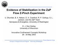
currently in operation (Fig. 1.1), but as this number increases it may be necessary to develop
2<br />
Figure 1.1: A snapshot <strong>of</strong> the US airspace showing the magnitude <strong>of</strong> the air traffic control<br />
task (photo courtesy <strong>of</strong> NASA).<br />
automated algorithms to decrease the workload <strong>of</strong> human operators.<br />
<strong>Collision</strong> avoidance is a difficult and interesting problem in the study <strong>of</strong> control theory<br />
because the goal is fundamentally different from that <strong>of</strong> a classical control system. The vast<br />
majority <strong>of</strong> classical control problems (and their current nonlinear counterparts) demand<br />
the system attain a particular point in the state space (be it stationary or moving). Most<br />
<strong>of</strong> the methods for this type <strong>of</strong> task use asymptotic analysis, whereby the system can be<br />
said to approach the goal regardless <strong>of</strong> the starting position or the route taken. <strong>Collision</strong><br />
avoidance is completely different in that there is no inherent end goal. The goal instead is<br />
to not enter particular regions <strong>of</strong> the state space at any time. <strong>Collision</strong> avoidance therefore<br />
has the effect <strong>of</strong> making the allowable set in the state space nonconvex, and in the case <strong>of</strong><br />
avoiding moving vehicles, the set is also time varying. Adding these restrictions to the state<br />
space makes otherwise simple problems extremely difficult. One <strong>of</strong> the primary reasons is<br />
that transient response is difficult to completely characterize using classical control, yet it<br />
is exactly these transients that cause most collisions. Now, instead <strong>of</strong> only considering the
3<br />
system state as time goes to infinity, one has to consider the system state at all times.<br />
When one factors in the highly nonlinear nature <strong>of</strong> the nonholonomic dynamics that<br />
govern most real vehicles, the problem truly balloons in complexity. Control authority limitations<br />
become far more important than in most classical control problems because control<br />
saturation primarily affects transient behavior. When two vehicles are on a collision course,<br />
it is exactly that transient behavior that determines their ability to avoid each other. If saturation<br />
is not accounted for explicitly, then collision avoidance becomes a trivial problem<br />
where a vehicle simply applies infinite control in the direction away from a collision. Of<br />
course this concept is unrealistic in practice, but nonetheless, many papers have been written<br />
on collision avoidance which rely on exactly this principle for their pro<strong>of</strong>s.<br />
The typical goal for designing a nonlinear control algorithm is to prove global asymptotic<br />
stability. Unfortunately, guaranteed global collision avoidance does not exist because<br />
all real vehicles have inertia and control authority limits, which place fundamental limits on<br />
their safe set <strong>of</strong> initial conditions. Two vehicles heading towards each other can always be<br />
placed close enough that nothing can be done to avoid a collision. Therefore no approach<br />
can possibly guarantee collision avoidance for arbitrary initial conditions. Determining the<br />
exact set <strong>of</strong> initial conditions for which avoidance is impossible becomes extremely complex<br />
as the number <strong>of</strong> vehicles increases, so generally the best that can be done is to define<br />
a bound or test, which if passed, yields a conservative guarantee.<br />
1.1 Definitions <strong>of</strong> Terms<br />
A wide range <strong>of</strong> methods have attempted to solve the collision avoidance problem, and<br />
the authors <strong>of</strong> a survey paper [5] split those methods into three categories: prescribed,<br />
optimized, and force field. In prescribed maneuver approaches, all vehicles follow a set<br />
protocol, not unlike the rules <strong>of</strong> the road. This approach tends to yield a discrete event<br />
controller, which when combined with the vehicle’s continuous dynamics, forms a hybrid<br />
system. Optimization methods attempt to find the best route for all the vehicles to take to<br />
avoid each other while minimizing a cost function. Generally, these methods use a look-
4<br />
ahead or time horizon so that the solution does not have to be recalculated <strong>of</strong>ten. Force field<br />
approaches use continuous feedback mechanisms to compute the control. Commonly, the<br />
force field between two vehicles is akin to the repulsion between two like-charged particles,<br />
however there are many possible alternatives for feedback schemes. These approaches are<br />
generally reactive, in that the control reacts to the current state <strong>of</strong> the system, rather than<br />
planning a trajectory ahead <strong>of</strong> time.<br />
The next differentiator between collision avoidance algorithms is their degree <strong>of</strong> centralization.<br />
Centralized means that all <strong>of</strong> the information about the vehicles is sent to a<br />
single server where the controls are calculated for each vehicle and sent back. The current<br />
air traffic control system uses centralization (with human operators), as do most optimization<br />
schemes. The other extreme is decentralization, in which no central server exists and<br />
each vehicle computes its own control based only on other vehicles within a particular range<br />
<strong>of</strong> itself. This situation is ideal from a computational perspective because there is a limit to<br />
how many vehicles can be within range at once, and therefore there is a limit to how much<br />
time the algorithm will take to run, regardless <strong>of</strong> the total number <strong>of</strong> vehicles involved. In<br />
between is a category termed distributed, in which there is still no central server and each<br />
vehicle computes its own control but may need more than local information to do so. In this<br />
case, computations scale with the number <strong>of</strong> vehicles involved (n), but the scaling is at least<br />
O(n) better than the centralized case, because now n separate processors are computing in<br />
parallel, rather than one server doing all the work.<br />
The vehicle model used in each formulation is also <strong>of</strong> utmost importance to the algorithm’s<br />
applicability to real systems. First, for collision avoidance to be nontrivial, the<br />
dynamics must be at least second order (acceleration-level control input), and the control<br />
inputs must be bounded to model the difficulties <strong>of</strong> overcoming inertia. Many vehicles<br />
(cars, ships, airplanes, etc.) have nonholonomic constraints, and as such are <strong>of</strong>ten modeled<br />
at a high level by unicycle dynamics. The inputs to this model are forward acceleration<br />
and heading rate (which is equivalent to acceleration normal to the velocity). All vehicles<br />
have a maximum speed, but some vehicles (notably airplanes) also have a positive min-
5<br />
imum speed. The constant-speed unicycle is one <strong>of</strong> the most broadly applicable vehicle<br />
models because it is the most constrained (less constrained vehicles can still duplicate its<br />
movements, but not vice-versa). Ideally an algorithm should use all <strong>of</strong> the capabilities a<br />
vehicle has to <strong>of</strong>fer, but still function under the constraints <strong>of</strong> a constant-speed unicycle if<br />
necessary.<br />
Another important aspect <strong>of</strong> a collision avoidance algorithm is whether it works for<br />
a heterogeneous group <strong>of</strong> vehicles. Heterogeneity can be due to differences in vehicle<br />
size, dynamics, speed range, control authority, etc. Many algorithms are developed for a<br />
homogeneous group <strong>of</strong> vehicles for convenience and ease <strong>of</strong> notation, but could be easily<br />
extended to a heterogeneous case. Others, especially constant-speed algorithms, can have<br />
difficultly generalizing from a homogeneous scenario. Another important consideration is<br />
that vehicle size, maximum speed, and control authority are <strong>of</strong>ten important parameters<br />
for the other vehicles in the system to know in order to properly avoid each other. In a<br />
homogeneous system these parameters are known implicitly because they are the same<br />
for every vehicle, but in a heterogeneous system, these parameters must be exchanged.<br />
Communication is the most obvious tool, though sensors could be employed to identify<br />
the vehicle type and compare it to some known list, the same way a captain can identify a<br />
sailboat or a ferry and infer their size and maneuverability. Until such technology is fully<br />
mature, heterogeneity may require some degree <strong>of</strong> inter-vehicle communication.<br />
A final aspect important to collision avoidance is liveness, which denotes the ability<br />
<strong>of</strong> the vehicles to attain their goals. Liveness is important to consider because one simple<br />
way to avoid collisions is to have everyone stop moving. While this method may avoid<br />
collisions, it is not useful because the vehicles cannot arrive at their destinations. This type<br />
<strong>of</strong> situation is called a deadlock. Another problem scenario is a livelock, where the vehicles<br />
continue to move, but in such a way that they cannot reach their goals.
6<br />
1.2 Literature Review<br />
Much work has been done on the collision avoidance problem to date, and a wide variety<br />
<strong>of</strong> solutions have been proposed. While each <strong>of</strong> these answers solves a piece <strong>of</strong> the puzzle,<br />
they also have limitations that keep them from solving the wide range <strong>of</strong> applications that<br />
the work in this dissertation seeks to address. However, they also form the foundation <strong>of</strong><br />
tools and ideas on which this work has been built.<br />
An early theoretical work on collision avoidance [6] showed a method <strong>of</strong> designing<br />
avoidance controllers for a general class <strong>of</strong> vehicle models and constraints. The mathematical<br />
foundation is solid in that it presents a pro<strong>of</strong> to avoid not just another vehicle, but<br />
an adversary. The method is limited because it requires finding an appropriate Lyapunov<br />
function, which is <strong>of</strong>ten a nontrivial task, and it only works for two-vehicle systems.<br />
The collision cone concept, introduced in [7] and subsequently used in the deconfliction<br />
literature [8, 9, 10, 11, 12], is a first order look ahead for detecting conflicts. The collision<br />
cone is a set <strong>of</strong> velocities for one vehicle that will cause it to collide with another, assuming<br />
each <strong>of</strong> their velocities are constant. While most algorithms using the collision cone define<br />
collision by the distance between two points (as though each vehicle is a disk or sphere),<br />
[7] shows how the method also works for irregularly shaped objects. An extension <strong>of</strong> the<br />
collision cone concept to accelerating vehicles was shown in [9], but the resulting conflict<br />
region is nonlinear and difficult to describe analytically, which limits its use for collision<br />
avoidance.<br />
A three-dimensional version <strong>of</strong> the original collision cone was used in [10] to avoid<br />
conflicts pairwise. Separate solutions were found using speed changes, heading changes,<br />
and flight path angle changes, but not in combination. An extension <strong>of</strong> that work to handle<br />
simultaneous speed, heading, and flight path angle changes was shown in [11]. Extensive<br />
real-world simulations were shown for two aircraft, but the algorithm is not designed for<br />
larger numbers <strong>of</strong> interacting vehicles.<br />
An application <strong>of</strong> the collision cone to three-dimensional air traffic control is presented
7<br />
in [12], where the rates <strong>of</strong> change <strong>of</strong> the collision cones are used to prioritize the evasion <strong>of</strong><br />
potentially adversarial vehicles. However, the protocols for handling multiple vehicles are<br />
not completely described, and no guarantees are given for safety, even in the two vehicle<br />
case.<br />
A combination <strong>of</strong> repulsive and vortex functions are used as force fields in [13], causing<br />
vehicles to form roundabout avoidance maneuvers, as tend to crop up in many <strong>of</strong> the collision<br />
avoidance methods. The algorithm provides no guarantees regarding safe separation,<br />
especially in the presence <strong>of</strong> control authority limits. Often parameters <strong>of</strong> the functions can<br />
be adjusted to give adequate results for a given situation, but it is unclear how to choose<br />
these parameters in general.<br />
A function involving more look-ahead is presented in [14], which shows good qualitative<br />
performance, but again lacks guarantees. Their simulations consistently show a significant<br />
percentage <strong>of</strong> the vehicles violating their separation bounds. A somewhat similar<br />
approach was taken by this author in [15], which avoided three dimensional conflicts by<br />
maneuvering out <strong>of</strong> the plane <strong>of</strong> the conflict. Again, simulations showed promise, but no<br />
guarantees could be found for safety.<br />
Gyroscopic and braking forces are used for collision avoidance in [16], resulting in a<br />
decentralized control law. However, safety can only be guaranteed so long as each vehicle<br />
only sees one other vehicle at a time within the detection range. Therefore no guarantees<br />
exist for systems with more than two vehicles, though simulations are shown for manyvehicle<br />
cases.<br />
A simple potential function method is employed for collision avoidance in [17], while<br />
simultaneously attaining a desired formation <strong>of</strong> the agents involved. The guarantee <strong>of</strong> collision<br />
avoidance given proves that the vehicles never attain the exact same position at the<br />
same time by using unbounded control authority. Problematically, no minimum separation<br />
distance or any concept <strong>of</strong> vehicle size is used in this method.<br />
Another force field approach that guarantees collision avoidance is presented in [18].<br />
Unfortunately, the guarantee is based on a potential function that goes to infinity at the mini-
8<br />
mum vehicle separation. Effectively, for the guarantee to apply, the vehicle must be capable<br />
<strong>of</strong> infinite control authority, which is an unreasonable assumption for any real vehicle.<br />
A realistic situation in which force-field collision avoidance is necessary is given in<br />
[19]. The idea is to use electrostatic charges on spacecraft to create enough repulsion force<br />
to avoid collisions in high orbit and deep space. This situation results in a different kind<br />
<strong>of</strong> underactuated system, but one for which collision avoidance is guaranteed, even in the<br />
case <strong>of</strong> control saturation, given restrictions on the initial conditions. These results use a<br />
Lyapunov function and only apply to the two-vehicle case.<br />
The work in [20] uses a navigation function to combine the tasks <strong>of</strong> collision avoidance<br />
and waypoint navigation into a single gradient-following routine. The navigation function<br />
is useful in its ability to guarantee liveness in a static environment. Unfortunately, adequate<br />
separation is not proven because the dynamics <strong>of</strong> the vehicle make it unable to follow the<br />
gradient in all cases. A vortex is added to the function to better the heuristic performance,<br />
but its effect on safety is unclear.<br />
A collision avoidance approach for a three-dimensional unicycle model that uses dipole<br />
navigation functions to avoid static obstacles while maneuvering to a goal is presented in<br />
[21]. While the dipole navigation functions provide smooth controls for the vehicle, still no<br />
way is given to choose the parameters such that particular rate limits are observed. These<br />
control limits can therefore cause collisions in certain situations.<br />
A high-performance force-field method is presented in [22], which uses a concept similar<br />
to an abbreviated collision cone to take into account how much space an avoidance<br />
maneuver will need based on the relative velocity between the vehicles. Simulations show<br />
promising results for large numbers <strong>of</strong> vehicles, and the computation time is kept low by<br />
the decentralized nature <strong>of</strong> the algorithm. While this algorithm does guarantee safety for a<br />
homogeneous system <strong>of</strong> two or three vehicles with acceleration constraints, its performance<br />
in larger systems is heuristic, and it does not allow unicycle-type dynamics in its vehicle<br />
model.<br />
The optimization scheme presented in [23] is performed over the reachable set <strong>of</strong> a
9<br />
hybrid system that describes each aircraft involved. Safety is guaranteed, but only in the<br />
two-vehicle case. An n-vehicle optimization approach is presented in [8] that uses a relaxation<br />
approach to turn the collision avoidance problem into a semidefinite program, solved<br />
with convex optimization. This achievement is impressive given the highly nonconvex<br />
nature <strong>of</strong> collision avoidance. Unfortunately, the solution must be centralized, and the algorithm<br />
is randomized, which means that to get an optimal solution, the optimization must<br />
be run several times. While convex optimization is computationally efficient compared to<br />
general nonlinear optimization, it is still less scalable than prescribed maneuver or force<br />
field approaches.<br />
A method showing better computation time is presented in [24], which uses mixed<br />
integer programming. This method allows for either speed changes or heading changes,<br />
but not both concurrently. It is still a centralized solution, and like many <strong>of</strong> the other<br />
optimization approaches, no mention is made <strong>of</strong> restrictions on the initial conditions to<br />
ensure that a feasible solution exists.<br />
Another convex relaxation approach to optimizing collision avoidance is shown in [25]<br />
for an n-spacecraft system using 3D double integrator dynamics. The algorithm works by<br />
computing an optimal set <strong>of</strong> new velocities each time any vehicles get too close together.<br />
These new velocities cause the vehicles to bounce away from each other, and in this way<br />
collision avoidance is guaranteed for the system as is liveness <strong>of</strong> the solution. However,<br />
in addition to the optimization being centralized, the control is designed to attain the new<br />
velocity in a single time step, meaning the magnitude <strong>of</strong> the control force is unbounded<br />
as the time step goes to zero. Alternatively, one could choose the time step to enforce a<br />
control limit, but given the discrete time nature <strong>of</strong> the constraints, motion during the time<br />
step would become significant and could cause collisions.<br />
An approach to distributing an optimization scheme across the vehicles involved is<br />
presented in [26]. This approach is much broader than collision avoidance, as the optimization<br />
occurs across a whole host <strong>of</strong> constraints, from visiting targets to avoiding danger<br />
zones. The authors use market-based task trading and evolutionary optimization to find
10<br />
paths dynamically for the vehicles. While most <strong>of</strong> the computations are distributed, a central<br />
server is still required to make the trades. Additionally, no guarantee has been made<br />
that a collision-free set <strong>of</strong> paths will be found.<br />
The authors <strong>of</strong> [27] also use a negotiation process to optimize collision avoidance maneuvers,<br />
but another algorithm must be present to give collision-free paths for the vehicles<br />
to start from for the guarantees to work. The idea is that this other algorithm need not be<br />
optimal, but merely feasible. Then the second stage enables the vehicles to negotiate a more<br />
optimal solution derived from the first. The algorithm for finding a set <strong>of</strong> feasible paths is<br />
not given, assuming instead that one <strong>of</strong> the other approaches discussed here will suffice.<br />
A major improvement in the computation time <strong>of</strong> optimization methods is shown in<br />
[28], which uses satisficing game theory to make a truly decentralized optimization scheme.<br />
This algorithm is efficient enough to make real-time computation reasonably scalable to<br />
large numbers <strong>of</strong> vehicles. The price paid for efficient computation is a loss <strong>of</strong> the safety<br />
guarantees, as simulation results show that collisions are rare, but that they do occur.<br />
In [29], a distributed collision avoidance algorithm with guaranteed safety is presented<br />
for a homogeneous group <strong>of</strong> n aircraft. This prescribed maneuver approach involves two<br />
discrete heading and speed changes for each aircraft, where each aircraft turns the same<br />
way. The method is based upon perturbations from an exact conflict, where all vehicles<br />
are headed toward a single collision point. This algorithm was extended in [30] to work in<br />
3D and to account for bounded acceleration. Since the algorithm is computed only once,<br />
it is unclear how it could account for a dynamically changing environment where vehicles<br />
are not necessarily capable <strong>of</strong> performing the exact maneuver prescribed. Additionally, the<br />
algorithm may run into trouble with extremely inexact conflicts, since it is based upon a<br />
transformation to an exact conflict.<br />
Probably the safest collision avoidance algorithm to date is that <strong>of</strong> [31], which considers<br />
a homogeneous group <strong>of</strong> constant-speed unicycles. This method uses a completely decentralized,<br />
prescribed maneuver algorithm for n vehicles which has an absolute guarantee <strong>of</strong><br />
safety in the presence <strong>of</strong> constrained control authority. While this solution might appear
11<br />
at first to be the holy grail <strong>of</strong> collision avoidance, it has some undesirable performance<br />
characteristics. To achieve this guarantee, the vehicles must keep a region the size <strong>of</strong> their<br />
turning diameter free <strong>of</strong> other vehicles at all times. For mobile robots this requirement may<br />
be reasonable, but for aircraft and ships that tend to have a turning radius much larger than<br />
their physical size, this requirement becomes overly conservative. Additionally, the system<br />
can suffer from deadlocks and livelocks.<br />
1.3 Introduction to DRCA<br />
The <strong>Distributed</strong> <strong>Reactive</strong> <strong>Collision</strong> <strong>Avoidance</strong> (DRCA) algorithm presented here fills an<br />
important gap in the current collision avoidance literature. Namely, this algorithm presents<br />
a distributed, computationally efficient method to guarantee collision avoidance between n<br />
vehicles in the presence <strong>of</strong> arbitrary control authority limitations. Plus, liveness <strong>of</strong> the solutions<br />
can be guaranteed, as well as robustness to modeling errors and adversarial behavior.<br />
The vehicle model used for the formulation <strong>of</strong> the problem is the 3D double-integrator.<br />
Specific vehicles are then modeled by restricting the control authority in particular directions<br />
by time- or state-dependent functions, rather than by adjusting the dynamics themselves.<br />
In this way, this single model can represent two-dimensional systems, or even<br />
nonholonomic vehicles <strong>of</strong> the constant-speed unicycle variety. Likewise, static obstacles<br />
can be avoided since they can be represented as a vehicle with zero speed and zero control<br />
authority. Higher order dynamics (like an airplane banking to turn) can be accounted for<br />
with the robustness analysis.<br />
The DRCA algorithm is a two-step process, consisting <strong>of</strong> an optimization-based deconfliction<br />
maneuver, followed by the longer-term deconfliction maintenance phase, which is a<br />
reactive, force-field type approach. Both <strong>of</strong> the steps are based upon the collision cone concept.<br />
The optimization schemes are uniquely distributed and scale well computationally.<br />
Though they do not find a global optimum, they do guarantee finding a feasible solution<br />
under given restrictions on the initial conditions. The deconfliction maintenance controller<br />
ensures that the vehicles follow their arbitrary outer-loop controllers as much as possible
12<br />
without sacrificing safety. This framework also allows vehicles to be given different priorities,<br />
such that lower priority vehicles will make way for higher priority ones.<br />
This algorithm requires little (though nonzero) communication between vehicles, and<br />
can safely add new vehicles to the system as they reach sensor range. While the algorithm<br />
is distributed, it is not quite decentralized, in that all-to-all information is needed within a<br />
connected group. The information exchange can be easily implemented through a broadcast,<br />
and if there is enough bandwidth for vehicles to rebroadcast the information they<br />
receive, then a quasi-all-to-all topology can be achieved. The robustness analysis accounts<br />
for the corresponding time delays. Additionally, the algorithm can be run in a completely<br />
decentralized fashion, and while some <strong>of</strong> the guarantees no longer apply, simulations are<br />
given that demonstrate significant capability nonetheless.<br />
No homogeneity is required among the vehicles that make up the system. The DRCA<br />
algorithm allows the vehicles to perform completely different tasks and to have different<br />
size, speed, actuation limitations, and control gains.<br />
The remainder <strong>of</strong> this dissertation is organized as follows. The problem statement is<br />
given in Chapter 2, including the vehicle model. Specific definitions <strong>of</strong> collision and the<br />
collision cone are given in Chapter 3. In Chapter 4 the DRCA algorithm is described, which<br />
forms the bulk <strong>of</strong> the dissertation. A robustness analysis is given in Chapter 5. Finally,<br />
simulation results are presented in Chapter 6 and concluding remarks in Chapter 7.
13<br />
Chapter 2<br />
PROBLEM STATEMENT<br />
The work here presents a method for deconflicting n vehicles.<br />
Each vehicle has a<br />
nominal desired control input, u d (t), which comes from an arbitrary outer-loop controller.<br />
This controller is designed for the vehicle to perform a desired task, which could range<br />
from target tracking to waypoint navigation, to area searching, etc. The goal <strong>of</strong> the DRCA<br />
algorithm is to adjust the control input on each vehicle to guarantee collision avoidance<br />
while simultaneously staying close to the desired control input (keeping in mind that this<br />
desired control can change with time).<br />
For this approach to collision avoidance, the only vehicle states that matter are position<br />
and velocity. Orientations affect performance, as they <strong>of</strong>ten have bearing on the magnitude<br />
<strong>of</strong> acceleration available in a particular direction, but they do not affect the underlying<br />
concepts <strong>of</strong> conflict and collision. In this way, many different vehicle models work equivalently<br />
with this approach. To simplify the math, a simple vehicle model will be used for<br />
most <strong>of</strong> the following analysis: a 3D double integrator, which for the i th vehicle is given by<br />
⎡ ⎤ ⎡ ⎤<br />
r<br />
d<br />
i v i<br />
⎢ v<br />
dt ⎣ i ⎥<br />
⎦ = ⎢ u<br />
⎣ i ⎥<br />
⎦ , (2.1)<br />
Θ i Ω i Θ i<br />
where r i , v i , u i ∈ R 3 are the position, velocity, and control input, respectively. The matrix<br />
Θ i<br />
= [ˆt i , ˆn i , ˆb i ] defines the orientation and Ω i is the cross product matrix <strong>of</strong> the body<br />
rotation vector ω = [ω t , ω n , ω b ] T . The notation throughout this paper will use bold face<br />
for vectors, hats over unit-vectors, script capital letters for sets, standard capital letters for<br />
matrices and functions, and everything else is assumed scalar. Quantities subscripted with<br />
t, n, or b refer to the tangent, normal, or binormal direction, respectively.
14<br />
Note that the orientation (defined by the ˆt, ˆn, and ˆb vectors) is only used as a local<br />
coordinate frame for the DRCA algorithm. The orientation does not directly affect the<br />
dynamics (r and v), and as such can be arbitrary. However, many vehicle’s input constraints<br />
are related to their orientation, and so it can be useful to tie this local coordinate frame to<br />
the actual body coordinates <strong>of</strong> the vehicle.<br />
We constrain the input by use <strong>of</strong> an arbitrarily varying constraint set, u i ∈ C i . The only<br />
requirement is that C i always contain the origin. A simple example <strong>of</strong> an input constaint set<br />
that limits maximum acceleration and velocity is<br />
C i =<br />
{<br />
u i ∈ R 3∣ }<br />
∣ ‖ui ‖ ≤ u max , ‖v i ‖ ≥ v max =⇒ u T i v i ≤ 0 . (2.2)<br />
For the DRCA algorithm, one must choose a set <strong>of</strong> rectangular constraints R i (which<br />
can also vary with time, state, etc.)<br />
for each vehicle that encloses its C i , as well as a<br />
corresponding saturation function, S i : R i → C i . The function S i must be continuous, must<br />
become the identity map for any u ∈ C i , and must preserve the sign <strong>of</strong> each component <strong>of</strong><br />
u when projected onto the ˆt, ˆn, and ˆb directions. In this example, one can choose<br />
R i = { u i ∈ R 3∣ ∣ − umaxi ≤ u ti ≤ u maxi , . . . } , (2.3)<br />
and<br />
⎧<br />
u<br />
u max i<br />
⎪⎨<br />
, ‖u ‖u i ‖ i‖ > u max<br />
S i = u i − v iu T i v i<br />
v max<br />
, ‖v i ‖ ≥ v max , u T i v i ≥ 0<br />
⎪⎩ u i , otherwise.<br />
(2.4)<br />
An example <strong>of</strong> how more complex vehicle dynamics can be represented by this simple<br />
model with an appropriate choice <strong>of</strong> input constraint set follows. Let us model a vehicle<br />
which can go forward with variable speed, can turn in two axes (a 3D unicycle model), and<br />
has limits on its turn rate, forward acceleration, and maximum speed. One way to describe<br />
the model mathematically is by
15<br />
⎡ ⎤ ⎡ ⎤<br />
r sˆt<br />
d<br />
⎢ s ⎥<br />
dt ⎣ ⎦ = ⎢ u<br />
⎣ a ⎥<br />
⎦ , (2.5)<br />
Θ ΩΘ<br />
where |u a | ≤ u amax , |ω n | ≤ ω nmax , |ω b | ≤ ω bmax , and |s| ≥ s max =⇒ u a s ≤ 0.<br />
Alternatively, an equivalent representation <strong>of</strong> the system is (2.1) with u = u aˆt+‖v‖ ω bˆn−<br />
‖v‖ ω nˆb. The tangent vector must be initialized to the same direction as the velocity vector,<br />
but the dynamics will keep them aligned from then on. In this case, R can be defined by<br />
u tmax = −u tmin = u amax<br />
u nmax = −u nmin = ‖v‖ ω bmax<br />
u bmax = −u bmin = ‖v‖ ω nmax , (2.6)<br />
and the accompanying saturation function is<br />
⎧<br />
⎪⎨ u − vuT v<br />
s<br />
S =<br />
max<br />
, ‖v‖ ≥ s max , u T v ≥ 0<br />
⎪⎩ u, otherwise.<br />
(2.7)<br />
Normally one would not equate a holonomic model to a nonholonomic one, largely<br />
because <strong>of</strong> differences in controllability. However, controllability is not essential to the<br />
DRCA algorithm since orientations are arbitrary, and only position and velocity matter.<br />
The DRCA algorithm is designed to use any control authority available, but it does not<br />
require the state space to be locally accessible.<br />
The relative position vector from vehicle i to vehicle j is denoted ˜r ij ≡ r j − r i , while<br />
the relative velocity vector is defined in the opposite sense: ṽ ij ≡ v i − v j . Note that these<br />
definitions imply that ˙˜r ij = −ṽ ij , and ˙ṽ ij = u i − u j .<br />
It is useful to define the dimensionless Deconfliction Difficulty Factor, η, to compare<br />
different systems in which collision avoidance is to be implemented. This factor is defined<br />
as<br />
η =<br />
v2 max<br />
u max d sep<br />
. (2.8)
16<br />
Conceptually, this factor is the ratio <strong>of</strong> the worst case turning radius to the required separation<br />
distance. It can also be thought <strong>of</strong> in terms <strong>of</strong> stopping distance.<br />
The DRCA algorithm was designed primarily for systems with large η (greater than<br />
unity) such as aircraft and ships, where the collision avoidance task is difficult because<br />
<strong>of</strong> the dominance <strong>of</strong> vehicle inertia. Vehicles with small η (significantly less than unity)<br />
such as mobile robots can <strong>of</strong>ten be modeled as having a direct velocity command, since<br />
the inertia becomes insignificant. In such cases, potential function methods for collision<br />
avoidance may be preferable to the DRCA algorithm because <strong>of</strong> their simplicity and ability<br />
to closely pack vehicles. The downside <strong>of</strong> potential function methods is their general lack<br />
<strong>of</strong> guarantees, especially when inertia is considered.
17<br />
Chapter 3<br />
CONFLICTS AND COLLISIONS<br />
The vehicles considered here are modeled as point masses, however physical vehicles<br />
have finite size. Therefore, to account for physical constraints in the theoretical model, the<br />
condition for collision is not to occupy the same position in space at the same time, but<br />
rather to come within a minimum allowed distance at some point in time. This minimum<br />
distance could be, for example, the five nautical mile separation between aircraft required<br />
by the FAA or the sum <strong>of</strong> the radii <strong>of</strong> two vehicles.<br />
Definition 1 (<strong>Collision</strong>). A collision occurs between vehicles i and j when<br />
‖˜r ij ‖ < d sep,ij , (3.1)<br />
where d sep,ij is the minimum allowed separation distance between the vehicles’ geometric<br />
centers.<br />
For two vehicles not actively in a collision, the next question is whether they will collide<br />
if they remain on their present headings. This situation will be called a conflict.<br />
Definition 2 (Conflict). A conflict occurs between vehicles i and j if they are not currently<br />
in a collision, but with zero control input (i.e. constant velocity), at some future point in<br />
time they will enter a collision:<br />
d min,ij min<br />
t>0 ‖˜r ij‖ < d sep,ij . (3.2)<br />
The following lemma provides a useful way to check for conflicts. To simplify the<br />
notation in the rest <strong>of</strong> this paper, the ij subscripts will generally be suppressed (for example,<br />
˜r ij will be written as ˜r).
18<br />
ṽ ij<br />
d sep,ij<br />
d sep,ij<br />
β<br />
Vehicle j<br />
α<br />
˜r ij<br />
α<br />
Vehicle i<br />
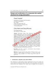
Figure 3.1: A 2D section <strong>of</strong> the collision cone along the ˜r ij -ṽ ij plane. The area between<br />
the two dotted lines is the collision cone; a conflict occurs when the relative velocity vector,<br />
ṽ ij , lies within this area.<br />
Lemma 1. Let β = ∠ṽ − ∠˜r 0 , α = arcsin<br />
( )<br />
dsep<br />
‖˜r 0<br />
and ˜r<br />
‖ 0 be the relative position vector<br />
at the time conflict is being checked. A necessary and sufficient condition for no conflict to<br />
occur is<br />
|β| ≥ α. (3.3)<br />
The angle α represents the half-width <strong>of</strong> the collision cone ([7, 8, 10]), which is depicted<br />
in Fig. 3.1.<br />
Pro<strong>of</strong>. First, define ˜r min as the position vector corresponding to the closest approach <strong>of</strong><br />
one vehicle to another in (3.2). By definition, at ˜r min the time derivative <strong>of</strong> ‖˜r‖ 2 = 0.<br />
Therefore:<br />
Next, note that for constant velocity, ṽ:<br />
d (˜rT˜r ) = 0<br />
dt<br />
ṽ T˜r min = 0. (3.4)<br />
˜r min = ˜r 0 − ṽt, (3.5)
19<br />
where t is the time to closest approach. To find t, multiply by ṽ T on both sides <strong>of</strong> (3.5),<br />
apply (3.4) and solve:<br />
ṽ T˜r min = ṽ T˜r 0 − ṽ T ṽt<br />
0 = ‖ṽ‖ ‖˜r 0 ‖ cos β − ‖ṽ‖ 2 t<br />
t = ‖˜r 0‖<br />
‖ṽ‖<br />
cos β. (3.6)<br />
Now, using (3.4), (3.5) and (3.6), a concise expression for the closest approach distance<br />
is given by<br />
d min =<br />
√<br />
˜r T min˜r min<br />
= √ (˜r 0 − ṽt) T˜r min<br />
√<br />
= ˜r T 0 (˜r 0 − ṽt)<br />
√<br />
=<br />
=<br />
‖˜r 0 ‖ 2 − ‖ṽ‖ ‖˜r 0 ‖ cos β<br />
√<br />
‖˜r 0 ‖ 2 (1 − cos 2 β)<br />
( ‖˜r0 ‖<br />
‖ṽ‖ cos β )<br />
= ‖˜r 0 ‖ |sin β| . (3.7)<br />
For no conflict to occur, the converse <strong>of</strong> (3.2) must be true:<br />
d sep ≤ d min<br />
= ‖˜r 0 ‖ |sin β| . (3.8)<br />
Therefore, to remain free <strong>of</strong> conflict it is necessary that:<br />
( )<br />
dsep<br />
|β| ≥ arcsin = α. (3.9)<br />
‖˜r 0 ‖<br />
exists.<br />
For sufficiency, if |β| ≥ α, then (3.9) and (3.8) still hold, thus implying that no conflict<br />
For notational simplicity below, ˜r 0 will be denoted simply by ˜r, as only its immediate<br />
value is used for the control (because the controller is reactive).
20<br />
Chapter 4<br />
DRCA ALGORITHM<br />
The DRCA algorithm uses a two-step process: a deconfliction maneuver and a deconfliction<br />
maintenance phase. The guarantees <strong>of</strong> n-vehicle collision avoidance rest upon three<br />
results. The first is that a deconfliction maneuver will keep the vehicles from colliding so<br />
long as they are each separated by at least a given bound. The second is that this deconfliction<br />
maneuver will result in a conflict-free state for the vehicles. The final result is that<br />
once a group <strong>of</strong> vehicles is conflict-free, the deconfliction maintenance controller will keep<br />
them that way.<br />
These steps yield the flow chart for the DRCA algorithm that is shown in Fig. 4.1.<br />
When the vehicles are sufficiently separated, no avoidance is necessary, so the vehicles<br />
can simply use their desired control. The deconfliction maintenance phase also takes the<br />
desired control into account, though there is no guarantee that it is followed at all times.<br />
In general, vehicles will not all see each other at the same time and perform one synchronous<br />
maneuver. Rather, they must avoid each other as they come into sensing/communication<br />
range (this will be referred to as communication from here on since some communication<br />
is required even if sensing is used). This maneuver does not require all-to-all communication,<br />
but does require some assumptions about connectivity and separation in order for the<br />
full collision avoidance guarantees to hold. However, if these assumptions are relaxed, the<br />
DRCA algorithm will still function as a high-performance heuristic, albeit without the full<br />
safety guarantee.<br />
The first step <strong>of</strong> the DRCA algorithm is to decide when a vehicle needs to perform its<br />
deconfliction maneuver. Let D be the set <strong>of</strong> vehicles who are currently deconflicting (either<br />
performing the deconfliction maneuver or deconfliction maintenance). Define a binary
21<br />
Enter<br />
Desired<br />
Control<br />
Deconfliction<br />
Maintenance<br />
Yes<br />
Yes<br />
Separated<br />
No<br />
Conflict−Free<br />
No<br />
Deconfliction<br />
Maneuver<br />
Figure 4.1: Flow chart <strong>of</strong> the DRCA algorithm.<br />
condition, χ i : D → {true,false}, which designates that the separation between vehicle<br />
i and the vehicles in D is enough to guarantee that vehicle i can avoid those vehicles. This<br />
condition will be derived later. Define a second binary condition, ξ i (D), which designates<br />
when vehicle i executes avoidance. The condition ξ i can be chosen for a longer or shorter<br />
look-ahead, but at the crossover point, χ i must be true.<br />
The DRCA algorithm causes vehicle i to follow its desired control until ξ i (D) becomes<br />
false. At this point vehicle i becomes a member <strong>of</strong> D and performs its deconfliction maneuver,<br />
which amounts to choosing a conflict-free velocity vector, broadcasting it to the<br />
group, and then accelerating to attain it as quickly as possible. Once this vehicle attains<br />
a conflict-free state with the other vehicles in D, it switches to deconfliction maintenance.<br />
The other vehicles in D that are already performing deconfliction maintenance avoid this<br />
new vehicle using its broadcast velocity instead <strong>of</strong> its actual velocity until its maneuver is<br />
complete. Conceptually, this method is akin to a turn signal, where the new vehicle tells<br />
the group how it will be accelerating, and the group can then work around that decision. As<br />
such, each vehicle will see no conflicts with a newly added member <strong>of</strong> the group. To implement<br />
this algorithm, each vehicle in D must be able to broadcast to all the other vehicles
22<br />
in D.<br />
If D is empty, then each vehicle uses ξ i (j) to determine when to maneuver, where j is<br />
the nearest vehicle. If vehicle i is less maneuverable than vehicle j, then ξ i (j) will turn<br />
false before ξ j (i) does. In this case, vehicle i becomes an element <strong>of</strong> D, making D = {i},<br />
but vehicle i does not perform a deconfliction maneuver, since vehicle j will be able to<br />
safely deconflict even if the vehicles move closer together. Now that D is nonempty, the<br />
system then follows the previous directions. Once ξ i (D) becomes true again, vehicle i is<br />
removed from D and solely follows its desired control.<br />
The deconfliction maneuvers used here are in fact simple optimization schemes with<br />
the goal <strong>of</strong> finding the smallest velocity change necessary to attain a conflict-free state.<br />
In this sense, the maneuvers are most similar to [8, 24] (in fact, because these authors’<br />
optimization schemes use the same definition <strong>of</strong> conflict, they could also be used as deconfliction<br />
maneuvers here). However, these two optimization schemes are centralized and<br />
computationally expensive. More importantly, they do not give a bound on how far apart<br />
the vehicles must be for a feasible solution to exist. This bound is <strong>of</strong> the utmost importance<br />
for designing a safe system.<br />
This algorithm is greedy in the sense that each vehicle minimizes its own cost function<br />
(‖∆v i ‖), meaning that the solution will not be a global optimum for some overarching cost<br />
function <strong>of</strong> the group. However, given the nonconvexity <strong>of</strong> the problem, finding any global<br />
optimum is nontrivial. For instance [8] used a semidefinite relaxation, but still required a<br />
random initial guess, and hence could not guarantee a global optimum either. Additionally,<br />
the actual cost function for the system is unknown in general, since any desired controller<br />
can have its own unique cost function associated with it, depending on the task. Therefore,<br />
instead <strong>of</strong> attempting to minimize an arbitrary cost function, a suboptimal solution will be<br />
allowed, with the focus instead on feasibility and low computation load.<br />
The only information the DRCA algorithm needs on a continuous basis is the position<br />
and velocity <strong>of</strong> each vehicle in D, which can either come from broadcast communication<br />
(e.g. a transponder) or sensing (e.g. radar). If the system is heterogeneous, then the vehicles
23<br />
must know a bound on the maximum speed and the minimum separation distance <strong>of</strong> the<br />
other vehicles in D, which can be accomplished by a broadcast communication or vehicle<br />
identification. Finally, the vehicles must know who is in D, and must receive the intended<br />
velocity <strong>of</strong> any vehicle performing a deconfliction maneuver. This information cannot be<br />
attained through sensing, so some form <strong>of</strong> broadcast communication is necessary to disseminate<br />
it. Any vehicle not yet in D only needs the information at a range just outside <strong>of</strong><br />
where ξ i (D) becomes false. In the case <strong>of</strong> D being empty, this information is required only<br />
<strong>of</strong> the nearest vehicle.<br />
There are two caveats with respect to the assumptions in this algorithm. First, two<br />
separate deconfliction groups cannot safely merge. The reason is that vehicles performing<br />
deconfliction maintenance are in general separated by as little as d sep , for which χ i (D) is<br />
false, but vehicles joining D must have χ i (D) true.<br />
In many applications, vehicles are added to a group singly. For example in an airport,<br />
if one considers the congested airspace <strong>of</strong> the airport itself as a group, wherein all vehicles<br />
are in the deconfliction maintenance phase with each other, then new aircraft arrive from<br />
all around where the airspace is not as congested. These aircraft can safely integrate one at<br />
a time as long as they stay separated from each other by enough space such that when one<br />
joins D it does not cause χ i (D) <strong>of</strong> the others to become false.<br />
The second caveat concerns communication range. While the communication range<br />
must be chosen such that vehicle i can talk to vehicle j by the time ξ i (j) becomes false,<br />
this range only ensures that D is connected, not necessarily all-to-all. This problem can be<br />
overcome by having vehicles rebroadcast information they have received. This multi-hop<br />
method will tend to accrue more time delay, however the robustness analysis in Chapter 5<br />
shows how the algorithm can be made robust to these delays.<br />
4.1 Deconfliction Maneuvers<br />
The purpose <strong>of</strong> the deconfliction maneuver is to bring a vehicle to a conflict-free state as<br />
quickly as possible with a guarantee that no collisions will occur during this maneuver,
24<br />
given certain bounds on the separation. The separation bounds are necessary because a<br />
wide class <strong>of</strong> initial conditions exist for which collision avoidance is impossible, usually<br />
due to a lack <strong>of</strong> sufficient control authority.<br />
While the deconfliction maintenance phase can operate with arbitrarily small control<br />
authority, the deconfliction maneuver requires control authority to get out <strong>of</strong> conflict before<br />
a collision occurs. Therefore it is important when designing a maneuver that the vehicle<br />
will have sufficient control authority to complete it. The problem with using speed changes<br />
in the maneuver is that all vehicles have a maximum speed, so their control authority to<br />
accelerate forward goes to zero as this maximum speed is approached.<br />
Therefore, turning as a means <strong>of</strong> deconfliction is applicable to a wider range <strong>of</strong> vehicles,<br />
since there is almost never a maximum heading angle. In addition, most vehicles have<br />
more acceleration available in turning than in speeding up or slowing down, since the latter<br />
requires work and former does not. Vertical acceleration can be as easy as turning for a<br />
buoyant vehicle, or require a significant change in potential energy for a vehicle such as<br />
an airplane. Therefore it may be prudent to restrict some vehicles to a 2D deconfliction<br />
maneuver in order to ensure they are capable <strong>of</strong> completing it.<br />
Two deconfliction maneuvers will be presented here, first a constant-speed maneuver<br />
that nearly any vehicle is capable <strong>of</strong>, and second a variable speed maneuver that has better<br />
performance at the cost <strong>of</strong> computational complexity. Both <strong>of</strong> these maneuvers are 2D, but<br />
deconfliction maintenance works for 3D as well. In order to use these maneuvers in a 3D<br />
application one would have to project the vehicle’s positions and velocities onto the plane,<br />
perform the maneuver, then add back in the original vertical component to the resulting<br />
velocity. The guarantees <strong>of</strong> attaining conflict-freedom will still apply (though the solutions<br />
will be more conservative) and once deconfliction maintenance takes over, the 3D nature <strong>of</strong><br />
the system will be accounted for in a less conservative way.
25<br />
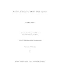
Figure 4.2: Example optimization <strong>of</strong> a constant-speed maneuver. The black vector is v i ,<br />
the red vector is v ′ i, the circle is the allowable space <strong>of</strong> solutions and the blue regions are<br />
the collision cones.<br />
4.1.1 Constant-Speed Maneuver<br />
The optimization vehicle i performs is to find a new velocity vector, v i, ′ which is free <strong>of</strong><br />
conflict with the other vehicles in D and minimizes ‖∆v i ‖, where ∆v i = v i ′ − v i . While<br />
this minimization is nonconvex in general (see Fig. 4.2), it can be solved relatively quickly<br />
because only a small number <strong>of</strong> possible points must be checked. The algorithm for solving<br />
this works as follows.<br />
The allowable space for v i ′ is a circle, centered at the origin, <strong>of</strong> radius ‖v i ‖. The collision<br />
cones split this space into several disjoint regions, each <strong>of</strong> which is an arc <strong>of</strong> the circle.<br />
The optimal solution to each region must lie on one <strong>of</strong> its two ends, unless there are no<br />
conflicts, in which case v i ′ = v i . The only possible end points are points where a collision<br />
cone intersects the allowable circle. Therefore the first step <strong>of</strong> the optimization is to calculate<br />
each <strong>of</strong> the intersections for each collision cone. This is done by first computing the<br />
unit-vector ĉ for each side, representing the direction <strong>of</strong> the edge <strong>of</strong> the collision cone (see
26<br />
Figure 3.1):<br />
where R is the 2 × 2 rotation matrix. Now v ′ i = v j − aĉ where<br />
a = ĉ T v j ±<br />
ĉ = R(±α) ˜r<br />
‖˜r‖ , (4.1)<br />
√<br />
(ĉ T v j ) 2 − v T j v j + v T i v i, (4.2)<br />
and only solutions with real and positive values <strong>of</strong> a are valid. The list <strong>of</strong> v is ′ are ordered<br />
by increasing ∆v i and checked consecutively for conflicts with the other vehicles. Because<br />
<strong>of</strong> the ordering, as soon as a point is found which is conflict free for all j, it is the optimal<br />
solution and the algorithm terminates.<br />
There are a finite number <strong>of</strong> points to check as possible optima, which bounds the<br />
maximum possible time the deconfliction maneuver will take to compute. For a vehicle<br />
deconflicting with n other members <strong>of</strong> D, there are a maximum <strong>of</strong> 4n points to check. Each<br />
<strong>of</strong> these much be checked against a maximum <strong>of</strong> n − 1 other collision cones. Therefore<br />
the maximum computation time is upper-bounded by cn 2 , where c is related to the time<br />
each type <strong>of</strong> computation requires. In general, the computation times are less than this<br />
bound because as soon as a feasible point is found, the algorithm terminates, so most points<br />
are never computed or checked. This bound is better than a general “polynomial time”<br />
guarantee (as with convex optimization, for instance), since in this case the polynomial is<br />
known to be quadratic.<br />
This analysis would guarantee a conflict-free solution if the vehicle could attain its<br />
desired velocity vector instantaneously. However, the limited control authority available<br />
makes this impossible. Instead, it takes a finite amount <strong>of</strong> time for the vehicle to attain<br />
its desired velocity, and during that time it and the other vehicles move, which causes the<br />
collision cones to move. In order to ensure that the system is still conflict-free after this<br />
motion, the initial collision cones must be enlarged to the point <strong>of</strong> enclosing all possible<br />
movements.<br />
To bound the collision cone, one must simply bound ‖∆˜r‖ ≤ δ, or how much the vehicles<br />
can change position before the maneuver is complete. Then the width <strong>of</strong> the collision
27<br />
cone is enlarged from (3.9) to<br />
( )<br />
dsep + δ<br />
α e = arcsin<br />
. (4.3)<br />
‖˜r‖<br />
Note that this expression implies an initial separation <strong>of</strong> ‖˜r‖ ≥ d sep + δ, or else α e will be<br />
undefined.<br />
Lemma 2. Let there be two vehicles (i and j), each modeled by a planar version <strong>of</strong> (2.1).<br />
Vehicle j is subject to the maximum speed constraint ‖v j ‖ ≤ v j,max . Vehicle i is subject<br />
to ‖u i ‖ ≤ u i,max and ‖v i ‖ constant and is turning as quickly as possible from its initial<br />
velocity, v i , to its desired velocity, v ′ i. The relative motion between the vehicles in the time<br />
it takes vehicle i to attain its desired velocity is bounded by ‖∆˜r‖ ≤ δ, where<br />
δ = ‖v i‖<br />
u i,max<br />
(2 ‖v i ‖ + πv j,max ) . (4.4)<br />
Pro<strong>of</strong>. The longest time, t, the maneuver could take is if v ′ i = −v i , so t ≤ π ‖v i ‖ /u i,max .<br />
Likewise, since vehicle i is tracing an arc, its motion is bounded by ‖∆r i ‖ ≤ 2 ‖v i ‖ 2 /u i,max .<br />
Finally, vehicle j is bounded by ‖∆r j ‖ ≤ v j,max t. Therefore,<br />
‖∆˜r‖ ≤ ‖∆r i ‖ + ‖∆r j ‖ ≤ 2 ‖v i‖ 2<br />
u i,max<br />
+ π ‖v i‖ v j,max<br />
u i,max<br />
= ‖v i‖<br />
u i,max<br />
(2 ‖v i ‖ + πv j,max ) . (4.5)<br />
This bound can in turn be used in (4.3) to size the enlarged collision cone. Note that for<br />
a homogeneous group <strong>of</strong> vehicles this bound can be written in terms <strong>of</strong> the deconfliction<br />
difficulty factor as δ = (2 + π)ηd sep . The following theorem states how this bound can be<br />
used to keep vehicles from colliding during a deconfliction maneuver.
28<br />
Theorem 1. Let there be a set <strong>of</strong> vehicles, D, which are not in conflict with each other.<br />
When another vehicle, i, is in conflict with some or all members <strong>of</strong> D and performs the<br />
constant-speed maneuver, the system will be conflict-free in time t, where<br />
t ≤ π ‖v i‖<br />
u i,max<br />
, (4.6)<br />
and no vehicles will collide during the maneuver. The vehicles are all modeled by a planar<br />
version <strong>of</strong> (2.1), have speed constraints ‖v j ‖ ≤ v j,max and vehicle i has the input constraint<br />
‖u i ‖ ≤ u i,max . It is assumed that a feasible solution to the optimization problem, v ′ i, exists<br />
and that the vehicles in D maintain a conflict-free state with v ′ i, using a cone with width<br />
defined by (4.3) and (4.4).<br />
Pro<strong>of</strong>. If a feasible point exists for the optimization problem, then the optimal solution is<br />
guaranteed to be found and this point will satisfy<br />
( )<br />
|∠ṽ ′ dsep + δ<br />
− ∠˜r| ≥ arcsin<br />
. (4.7)<br />
‖˜r‖<br />
The maximum amount <strong>of</strong> time required for vehicle i to get from its initial v i to v ′ i is t =<br />
π ‖v i ‖ /u i,max , and during this time ∆˜r ≤ δ from Lemma 2. Therefore, once the desired<br />
velocities have been attained, one still has<br />
|∠ṽ ′ − ∠(˜r + ∆˜r)| ≥ arcsin<br />
( )<br />
dsep<br />
, (4.8)<br />
‖˜r‖<br />
meaning the vehicles are not in conflict. The vehicles cannot collide during this time because<br />
as stated earlier, the pairs must be initially separated by at least ‖˜r‖ ≥ d sep + δ,<br />
which means after the maneuver, they still must be outside <strong>of</strong> collision because ‖˜r + ∆˜r‖ ≥<br />
d sep .<br />
Of course, all <strong>of</strong> this is for naught if a feasible solution does not exist for the optimization.<br />
The following theorem gives a conditional bound, χ i (D), on initial separation that is<br />
sufficient to guarantee the existence <strong>of</strong> a solution.
29<br />
Theorem 2. For vehicle i <strong>of</strong> an n-vehicle system in the plane, let vehicle i’s speed be<br />
the constant ‖v i ‖, while each other vehicle’s speed is constrained by the uniform bound<br />
‖v j ‖ ≤ v max . There exists an admissible velocity vector, v ′ i, which is conflict-free with the<br />
other n − 1 vehicles, given that vehicle i is separated from the other vehicles such that<br />
⎧ (<br />
∑<br />
√ )<br />
‖v<br />
⎪⎨ arccos cos(2α e ) − sin(2α e ) i ‖ 2<br />
− 1 , ‖v<br />
vmax<br />
2 i ‖ < v max<br />
j∈D<br />
π ≥<br />
(4.9)<br />
∑<br />
⎪⎩ 2α e , ‖v i ‖ ≥ v max .<br />
j∈D<br />
Pro<strong>of</strong>. In order for a conflict-free point to exist, the collision cones from the other vehicles<br />
cannot completely cover the admissible circle <strong>of</strong> possible headings <strong>of</strong> vehicle i. When<br />
another vehicle’s maximum speed is higher, the largest range <strong>of</strong> headings, θ, it can cover<br />
occurs when one edge <strong>of</strong> its collision cone is tangent to the admissible circle (see Fig. 4.3).<br />
Some geometry can show that the relationship between the width <strong>of</strong> the expanded collision<br />
cone, α e , and θ is given by<br />
⎛<br />
θ ≤ 2 arccos ⎝cos(2α e ) − sin(2α e )<br />
√<br />
‖v i ‖ 2<br />
v 2 max<br />
⎞<br />
− 1⎠ . (4.10)<br />
As long as the sum <strong>of</strong> those θs is less than 2π, then not all <strong>of</strong> the possible headings can be<br />
in conflict. When the other vehicle’s maximum speeds are less, then θ takes on its limiting<br />
value <strong>of</strong> 4α e . Putting this all together yields the full bound (4.9).<br />
4.1.2 Variable-Speed Maneuver<br />
If a vehicle has no minimum speed (i.e. it can stop), then it can use a variable-speed deconfliction<br />
maneuver, which has better performance than the constant-speed maneuver. The<br />
better performance comes from the fact that any constant-speed maneuver is admissible for<br />
a variable-speed vehicle, so this optimization is less constrained than the previous, meaning<br />
the solution must be equal to or better than the constant-speed solution. The cost <strong>of</strong> this<br />
optimality is higher computational load.
30<br />
Figure 4.3: Example <strong>of</strong> a borderline case for five vehicles where no conflict-free constantspeed<br />
maneuver exists. The circle is the allowable set (radius ‖v i ‖) and the blue regions<br />
are the collision cones (shown with all equal velocities, <strong>of</strong> magnitude greater than ‖v i ‖).<br />
The allowable space for v ′ i is a disk, centered at the origin, <strong>of</strong> radius v i,max . The optimal<br />
solution to each region must lie on its boundary because the zero-cost point is not<br />
feasible (otherwise there would be no conflicts). This optimal solution must either be a<br />
vertex between two collision cones, the nearest point on a single collision cone, or the vertex<br />
between one collision cone and the edge <strong>of</strong> the allowable space. An example <strong>of</strong> this<br />
optimization is shown in Fig. 4.4.<br />
The first step <strong>of</strong> the algorithm is to compute each <strong>of</strong> the nearest points on each collision<br />
cone (there is a right and a left solution for each cone), which is v ′ i = ĉĉ T ṽ + v j . This<br />
list <strong>of</strong> points is checked to make sure each ‖v ′ i‖ ≤ v i,max . If this is not the case, then v ′ i is<br />
replaced with<br />
√<br />
v i ′ = v j − ĉĉ T v j ± ĉ (ĉ T v j ) 2 − vj Tv j + vi,max 2 , (4.11)<br />
where only the solution with the smaller ∆v i is kept. These points account for the only<br />
possible optima on the intersection <strong>of</strong> a cone and the edge <strong>of</strong> the space. Next, all <strong>of</strong> the twocone<br />
intersection points are found using linear equations (keeping only those with ‖v ′ i‖ ≤<br />
v i,max ). All <strong>of</strong> these points are ordered by increasing ∆v i and checked consecutively for
31<br />
Figure 4.4: Example optimization <strong>of</strong> a variable-speed maneuver. The black vector is v i , the<br />
red vector is v ′ i, the circle is the edge <strong>of</strong> the allowable disk <strong>of</strong> solutions and the blue regions<br />
are the collision cones.<br />
conflicts with the other vehicles. Because <strong>of</strong> the ordering, as soon as a point is found which<br />
is conflict free for all j, it is the optimal solution and the algorithm terminates.<br />
As with the constant-speed maneuver, this optimization has a bound on its computation<br />
time since there are still a finite number <strong>of</strong> possible optima to check. However, since there<br />
are now points that are a combination <strong>of</strong> two cones, there are O(n 2 ) points to check. Since<br />
these still need to be checked for conflict with the other n−2 collision cones, the maximum<br />
computation time is now upper-bounded by cn 3 , rather than cn 2 , where c is related to the<br />
time each type <strong>of</strong> computation requires.<br />
Just as with the previous optimization, this algorithm usually terminates far before its<br />
maximum computation time. However, if a particular application has very little computational<br />
resource available, the constant-speed maneuver can still be used on a variable-speed<br />
vehicle. The solution will not in general be as optimal as the variable-speed maneuver, but<br />
it will be feasible and does scale better in computation time.
32<br />
Once again the time required to attain this new velocity vector must be accounted for<br />
in order to ensure the system actually comes to a conflict-free state and that there are no<br />
collisions. The following lemma parallels Lemma 2, but obtains a smaller bound by use <strong>of</strong><br />
the now 2D acceleration vector.<br />
Lemma 3. Let there be two vehicles (i and j), each modeled by a planar version <strong>of</strong> (2.1).<br />
Vehicle j is subject to the maximum speed constraint ‖v j ‖ ≤ v j,max . Vehicle i is subject to<br />
‖u i ‖ ≤ u i,max and ‖v i ‖ ≤ v i,max and is accelerating as quickly as possible from its initial<br />
velocity, v i , to its desired velocity, v ′ i. The relative motion between the vehicles in the time<br />
it takes vehicle i to attain its desired velocity is bounded by ‖∆˜r‖ ≤ δ, where<br />
δ = v i,max<br />
u i,max<br />
(v i,max + 2v j,max ) . (4.12)<br />
Pro<strong>of</strong>. Let the angle between v i and v ′ i be 2γ and let t be the time required for the maneuver.<br />
Then ‖∆v i ‖ = u i,max t, ‖∆r i ‖ = t ‖v i + v ′ i‖ /2, and ‖∆r j ‖ ≤ v j,max t. Also,<br />
‖v i + v ′ i‖ ≤ 2v i,max cos γ and ‖∆v i ‖ ≤ 2v i,max |sin γ|. Therefore,<br />
‖∆˜r‖ ≤ ‖∆r i ‖ + ‖∆r j ‖ ≤ 2v2 i,max |cos γ sin γ|<br />
u i,max<br />
+ 2v i,maxv j,max |sin γ|<br />
u i,max<br />
≤ v i,max<br />
u i,max<br />
(v i,max + 2v j,max ) . (4.13)<br />
This bound can in turn be used in (4.3) to size the enlarged collision cone. Note that for<br />
a homogeneous group <strong>of</strong> vehicles this bound can be written in terms <strong>of</strong> the deconfliction<br />
difficulty factor as δ = 3ηd sep . Also note that if one decides to use the constant-speed<br />
maneuver on a vehicle that fits the assumptions <strong>of</strong> Lemma 3, then one can still use the δ<br />
bound <strong>of</strong> (4.12), since the pro<strong>of</strong> is only based on the vehicle’s capabilities.<br />
Theorem 1 still applies to the variable-speed maneuver, with the slight adjustment <strong>of</strong><br />
(4.6) to t = 2v i,max /u i,max (see above). However, Theorem 2 requires some adjustments to<br />
the bound χ i (D):
33<br />
Theorem 3. For vehicle i <strong>of</strong> an n-vehicle system in the plane, let vehicle i’s speed be constrained<br />
by ‖v i ‖ ≤ v i,max , while each other vehicle’s speed is constrained by the uniform<br />
bound ‖v j ‖ ≤ v max . There exists an admissible velocity vector, v ′ i, which is conflict-free<br />
with the other n − 1 vehicles, given that vehicle i is separated from the other vehicles such<br />
that<br />
⎧ ( )<br />
∑<br />
⎪⎨<br />
vi,max<br />
arcsin<br />
v<br />
α e ≤<br />
max<br />
, v i,max < v max<br />
j∈D<br />
⎪⎩ π<br />
, v 2 i,max ≥ v max .<br />
(4.14)<br />
Pro<strong>of</strong>. In order for a conflict-free point to exist, the collision cones from the other vehicles<br />
cannot completely cover the admissible disk <strong>of</strong> possible velocities <strong>of</strong> vehicle i. The worst<br />
case for this coverage when the other vehicles are capable <strong>of</strong> higher speed than vehicle i is<br />
when all the vehicles have the same velocity, with their maximum speed, and their positions<br />
splay out their collision cones so as to form one large, continuous cone (see Fig. 4.5). The<br />
interior angle <strong>of</strong> this large cone must be less than 2 arcsin(v i,max /v max ) to ensure that it<br />
cannot cover the entire admissible circle. When vehicle i’s speed is higher than the other<br />
vehicles, the arcsine takes on its limiting value <strong>of</strong> π/2 and becomes conservative because<br />
it only allows the combined collision cone to cover a half-space within the disk. Together<br />
these constraints form (4.14).<br />
In the special case where all <strong>of</strong> the vehicles are exactly the same distance away (as in<br />
Fig. 4.5), the bound (4.14) can be simplified to a bound on distance. First note that the sum<br />
<strong>of</strong> the collision cones is just (n − 1)α e and rearranging (4.3) gives ‖˜r‖ ≥ (d sep + δ)/ sin α e .<br />
Then the distance bound is<br />
⎧<br />
⎪⎨<br />
‖˜r‖ ≥<br />
⎪⎩<br />
sin<br />
d sep+δ<br />
arcsin ( v i,max<br />
vmax )<br />
n−1<br />
d sep+δ<br />
π<br />
sin(<br />
!, v i,max < v max<br />
2(n−1)) , v i,max ≥ v max .<br />
(4.15)
34<br />
Figure 4.5: Example <strong>of</strong> a borderline case for six vehicles where no conflict-free variablespeed<br />
maneuver exists. The circle is the edge <strong>of</strong> the allowable disk (radius v i,max ) and the<br />
blue regions are the collision cones, shown with all equal velocities, <strong>of</strong> magnitude greater<br />
than v i,max .<br />
Note that for large n, the small angle approximation can be used to simplify (4.15) to<br />
⎧<br />
⎪⎨<br />
‖˜r‖ ≥<br />
⎪⎩<br />
(n−1)(d<br />
„ sep+δ)<br />
vi,max<br />
«,<br />
arcsin v j,max<br />
v i,max < v j,max<br />
2(n−1)<br />
π<br />
(d sep + δ), v i,max ≥ v j,max ,<br />
(4.16)<br />
however the result is not actually conservative, so (4.15) should still be used for safety<br />
purposes. It is interesting to note though, that as n gets large, the bound approaches a linear<br />
relationship with n − 1. This makes intuitive sense in that as more vehicles are in a space,<br />
they must be spaced out more to ensure a safe trajectory exists between them.<br />
4.1.3 Heuristic Performance<br />
The guarantees provided by the previous maneuvers are ideal if one can ensure the vehicles<br />
always have enough warning <strong>of</strong> each other’s presence. However, some systems may not<br />
always be that capable. We know from the previous analysis that these requirements are<br />
conservative, so it may still be possible to deconflict the system, though not in a guaranteed
35<br />
fashion. The goal then is to have a heuristic backup algorithm that will do a qualitatively<br />
good job <strong>of</strong> attempting to deconflict vehicles which do not meet the requirements <strong>of</strong> the<br />
guarantees. Handily, this heuristic backup algorithm can be seamlessly joined with the<br />
normal deconfliction maneuvers. Basically it operates the exact same way, but guarantees<br />
that a solution is returned regardless <strong>of</strong> feasibility.<br />
The first thing that could cause a solution to not exist is if ‖˜r‖ < d sep + δ, causing<br />
α e to be undefined. In this situation, let the heuristic be to define α e = π/2 (its limiting<br />
value). The only other thing that could cause a solution to not exist is if the collision cones<br />
cover the entire admissible space, making the optimization find no feasible solution. In this<br />
case, let the heuristic return the solution v i ′ = −v i . This solution was chosen because it is<br />
a velocity the vehicle can attain and it will take maximum acceleration to get there. The<br />
intuition behind the choice is that when vehicles are in conflict, it is better to do something<br />
than nothing, and by continuing to use maximum acceleration, there is more chance that<br />
the system will stumble upon a conflict-free state.<br />
The vehicle in this case does not join D until it attains a conflict-free state, since the<br />
deconfliction maintenance controller that the other vehicles in D are running cannot cope<br />
with vehicles in conflict. As a worst case, it is better for the new vehicle to collide with one<br />
<strong>of</strong> the members <strong>of</strong> D than to cause them all to collide with each other.<br />
Now the DRCA algorithm can be compared to other collision avoidance algorithms<br />
that are completely decentralized or have other assumptions that violate the requirements<br />
for guaranteed avoidance. Most <strong>of</strong> these algorithms are also heuristic, in that they do not<br />
guarantee collision avoidance in the presence <strong>of</strong> limited available acceleration and a minimum<br />
separation distance, d sep > 0. Therefore the algorithms can be compared qualitatively<br />
based on how <strong>of</strong>ten collisions occur and how well the vehicles attain their goals. This performance<br />
comparison is shown in Chapter 6.
36<br />
Desired<br />
Control<br />
u d<br />
Deconfliction<br />
Maintenance<br />
u<br />
Vehicle<br />
z i<br />
z<br />
Figure 4.6: Block diagram <strong>of</strong> the system when using the deconfliction maintenance controller.<br />
The vector z = [z 1 , z 2 , . . . , z n ] T and z i = [r i , v i ] T . Note that the deconfliction<br />
maintenance block acts as a type <strong>of</strong> saturation on the desired control, u d .<br />
4.2 Deconfliction Maintenance<br />
Once the deconfliction maneuver has been performed and the system is in a conflict-free<br />
state, then the deconfliction maintenance controller can be used to keep the system conflictfree.<br />
This controller allows each vehicle to use its desired control input unless that input<br />
would cause the vehicle to come into conflict with another vehicle. A basic block diagram<br />
<strong>of</strong> this setup is shown in Fig. 4.6.<br />
4.2.1 Control Law<br />
In order to smoothly transition from the desired control to the avoidance control, each<br />
vehicle needs a way to measure how close its velocity vector is to causing a conflict. The<br />
first step is to construct a unit-vector, ĉ, representing the side <strong>of</strong> the collision cone nearest<br />
ṽ (like (4.1), but now in 3D). The vector ĉ is found by rotating ˜r by α around a vector<br />
q = ˜r × ṽ and normalizing:<br />
ĉ =<br />
˜r ( ) q × ˜r<br />
‖r‖ cos α + sin α. (4.17)<br />
‖q‖ ‖r‖<br />
Next, construct a normal vector, e, from the collision cone to the relative velocity vector,<br />
ṽ (see Fig. 4.7). If ĉ T ṽ > 0, then e = (I − ĉĉ T )ṽ, but if ĉ T ṽ ≤ 0 (the vehicles are headed<br />
away from each other), then no normal exists, and the nearest point on the collision cone is
37<br />
v ĩ<br />
v<br />
e<br />
p t,ijˆt i<br />
v j<br />
p n,ijˆn i<br />
d sep<br />
ĉ<br />
β<br />
α<br />
˜r<br />
α<br />
d sep<br />
Figure 4.7: Geometry <strong>of</strong> the e and ĉ vectors, as seen in an ˜r-ṽ section through the 3D<br />
collision cone (dotted lines). The conflict measures p t and p n are shown, but ˆb points into<br />
the page, so p b is infinite (ĉ T ṽ > 0 in this example).<br />
the tip, so e = ṽ. Therefore:<br />
⎧<br />
⎪⎨ ṽ, ĉ T ṽ ≤ 0<br />
e =<br />
⎪⎩ (I − ĉĉ T )ṽ, ĉ T ṽ > 0.<br />
(4.18)<br />
In order to combine the effects <strong>of</strong> multiple collision cones, it is helpful to decompose<br />
the system into three component directions and analyze those directions separately. Let the<br />
coordinate system be defined by the orthonormal vectors ˆt, ˆn, and ˆb. The orientation <strong>of</strong> this<br />
coordinate system is arbitrary, but the convention <strong>of</strong> using tangent, normal, and binormal<br />
notation is chosen since fixing the coordinates to the body <strong>of</strong> the vehicle <strong>of</strong>ten simplifies<br />
analysis.<br />
The next step is to determine how much control (change in velocity) can be applied in<br />
each <strong>of</strong> these directions before a conflict forms. For simplicity, a conservative approach<br />
is taken whereby the signed distance is found from ṽ to the tangent plane enclosing the<br />
collision cone (defined by the normal vector e) in each <strong>of</strong> the ˆt, ˆn, and ˆb directions. These<br />
signed distances are<br />
p t,ij = ‖e ij‖ 2<br />
, p<br />
e T n,ij = ‖e ij‖ 2<br />
ijˆt i e T ijˆn , and p b,ij = ‖e ij‖ 2<br />
, (4.19)<br />
i<br />
e T ijˆb i
38<br />
which are described graphically in Fig. 4.7.<br />
Define ɛ t , ɛ n , ɛ b > 0 as thresholds such that when |p t | > ɛ t , the conflict is far enough<br />
away that it can be ignored (and likewise for p n and p b ). The n-vehicle deconfliction maintenance<br />
controller running on vehicle i computes p t , p n , and p b to each <strong>of</strong> the other vehicles<br />
and then finds the closest conflict in each direction, i.e.<br />
p + t i<br />
p − t i<br />
= min<br />
j∈D {p t,ij > 0, ɛ ti }<br />
= − max<br />
j∈D {p t,ij < 0, −ɛ ti } ,<br />
(4.20)<br />
and likewise for p n and p b . Note that by definition 0 < p ± ≤ ɛ. To simplify notation, in any<br />
case where a relation holds in the tangent, normal, and binormal directions, the subscript<br />
will be suppressed.<br />
The input is constructed using a function, F , such that in each direction u = F (p + , p − ).<br />
The control function chosen for this implementation <strong>of</strong> the DRCA algorithm is<br />
F (p + , p − ) = u min<br />
ɛ<br />
p + + u max<br />
p − + u d − u max − u min<br />
p + p − , (4.21)<br />
ɛ<br />
ɛ 2<br />
because it is a bilinear interpolation <strong>of</strong> the following ordered triples <strong>of</strong> the form (p + , p − , u):<br />
P 1 = (0, 0, 0) P 2 = (ɛ, 0, u min )<br />
P 3 = (0, ɛ, u max ) P 4 = (ɛ, ɛ, u d ).<br />
(4.22)<br />
An example <strong>of</strong> this control function is shown in Fig. 4.8. Because F depends on the desired<br />
control, u d must be saturated such that<br />
u min ≤ u d ≤ u max . (4.23)<br />
This choice <strong>of</strong> control function means that once the u vector is constructed from its<br />
three components, then u ∈ R. Then the saturation function S will give the final resultant<br />
control vector, which will be in C. The octant-preserving nature <strong>of</strong> S will ensure this final<br />
saturation step does not violate the requirements for the pro<strong>of</strong> <strong>of</strong> collision avoidance.<br />
A more intuitive way to choose values for ɛ is to relate it to a gain-like parameter,<br />
k = u max − u min<br />
. (4.24)<br />
ɛ
39<br />
Figure 4.8: Example <strong>of</strong> the control function, F . Note that P 4 moves up and down with<br />
changing u d .<br />
Note that k has units <strong>of</strong> inverse seconds. Also, one can see that the magnitude <strong>of</strong> the<br />
gradient <strong>of</strong> the control function will always be less than or equal to k, regardless <strong>of</strong> the<br />
desired control.<br />
Assuming there are n vehicles in the deconfliction group, D, this algorithm’s computation<br />
time on each vehicle scales as O(n), since it only requires the computation <strong>of</strong> each<br />
other vehicle’s collision cone and then substituting these results into the control function.<br />
Technically there are O(n 2 ) computations happening in the entire group, but since these<br />
computations are independent <strong>of</strong> each other (only linked by the sensed or communicated<br />
states), they can happen in parallel in a distributed fashion, so only the per-vehicle scaling<br />
matters.<br />
4.2.2 Guarantee<br />
The following theorem and pro<strong>of</strong> guarantee that the system can maintain its conflict-free<br />
state despite arbitrary control authority restrictions. Each time a new vehicle is added to the
40<br />
deconfliction group, D, it performs its deconfliction maneuver, broadcasting a conflict-free<br />
velocity to the group. Since it is this broadcasted velocity that is used by the deconfliction<br />
maintenance algorithm until the new vehicle really is conflict-free, the deconfliction group<br />
never sees any new conflicts.<br />
Theorem 4. The deconfliction maintenance controller described above, when implemented<br />
on n vehicles with dynamics (2.1) and inputs constrained by C i , will keep the system collision<br />
free for all time if the system starts conflict-free.<br />
Pro<strong>of</strong>. To measure the distance to a collision, define m as a signed version <strong>of</strong> ‖e‖ (in terms<br />
<strong>of</strong> ṽ from the geometry in Fig. 4.7):<br />
⎧<br />
⎪⎨ ‖ṽ‖ , ĉ T ṽ ≤ 0<br />
m =<br />
⎪⎩ ‖ṽ‖ sin(|β| − α), ĉ T ṽ > 0.<br />
Note that m is negative during conflict and positive during no conflict.<br />
(4.25)<br />
To ensure that a conflicted state is never reached (i.e. m is always greater than zero), it<br />
is sufficient to show that for every pair <strong>of</strong> vehicles there is a neighborhood on the positive<br />
side <strong>of</strong> m = 0 where ṁ ≥ 0. This condition implies that as the boundary <strong>of</strong> a collision cone<br />
approaches, it will either stop approaching or recede before a conflict is formed. The fact<br />
that this is a one-sided neighborhood is important because ṁ does not exist at m = 0 for<br />
the same reason that d ‖ṽ‖ does not exist at ṽ = 0. However, if this condition is satisfied,<br />
dt<br />
then m > 0 for all time, ensuring that m ≠ 0.<br />
For ĉ T ṽ ≤ 0 (using the ij notation again briefly for clarity),<br />
ṁ = eT ˙ṽ<br />
m = êT ˙ṽ, (4.26)<br />
where ê = e<br />
‖e‖ . Expanding u i into its components yields u i = [u ti t i + u ni n i + u bi b i ]. Next<br />
substitute for ṽ ij in (4.26) to get<br />
ê T ij ˙ṽ ij = u ti ê T ijˆt i + u ni ê T ijˆn i + u bi ê T ijˆb i − u tj ê T ijˆt j − u nj ê T ijˆn j − u bj ê T ijˆb j . (4.27)
41<br />
Because <strong>of</strong> the symmetry <strong>of</strong> the problem e ji = −e ij , so<br />
ê T ˙ṽ ij ij =u ti ê T ijˆt i + u ni ê T ijˆn i + u bi ê T ijˆb i + u tj ê T jiˆt j + u nj ê T jiˆn j + u bj ê T jiˆb j<br />
(<br />
uti<br />
=m ij + u n i<br />
+ u b i<br />
+ u t j<br />
+ u n j<br />
+ u )<br />
b j<br />
. (4.28)<br />
p t,ij p n,ij p b,ij p t,ji p n,ji p b,ji<br />
For ĉ T ṽ > 0, the derivative <strong>of</strong> (4.25) becomes<br />
ṁ = sin(|β| − α) d ‖ṽ‖<br />
dt<br />
+ ‖ṽ‖ cos(|β| − α) d (|β| − α). (4.29)<br />
dt<br />
The derivative exists because m > 0 implies ‖ṽ‖ ≠ 0, |β| ≥ α > 0, and ‖˜r‖ ≥ d sep > 0.<br />
From the geometry,<br />
d |β|<br />
dt<br />
( d∠ṽ<br />
= sgn(β) − d∠˜r )<br />
dt dt<br />
= sgn(β) d∠ṽ<br />
dt<br />
The derivative <strong>of</strong> α is somewhat less straight-forward:<br />
dα<br />
dt = d ( ( ))<br />
dsep<br />
arcsin<br />
dt ‖˜r‖<br />
= d dt<br />
( ) (<br />
dsep<br />
1 −<br />
‖˜r‖<br />
⎛<br />
= d sep ‖ṽ‖ cos β<br />
‖˜r‖ 2<br />
Combining the above two terms gives<br />
+ ‖ṽ‖ |sin β| . (4.30)<br />
‖˜r‖<br />
( ) ) 2 −1/2<br />
dsep<br />
‖˜r‖<br />
⎞<br />
⎝<br />
‖˜r‖<br />
√ ⎠<br />
‖˜r‖ 2 − d 2 sep<br />
= ‖ṽ‖ cos β tan α. (4.31)<br />
‖˜r‖<br />
d<br />
‖ṽ‖<br />
(|β| − α) = (|sin β| − cos β tan α) + sgn(β)d∠ṽ<br />
dt ‖˜r‖ dt , (4.32)<br />
which can be substituted into (4.29) to get<br />
ṁ = sin(|β| − α) d ‖ṽ‖<br />
dt<br />
+ cos(|β| − α) sgn(β) ‖ṽ‖ d∠ṽ<br />
dt<br />
+ cos(|β| − α) ‖ṽ‖2 (|sin β| − cos β tan α). (4.33)<br />
‖˜r‖
42<br />
To simplify the above, note that in the case <strong>of</strong> ĉ T ṽ > 0, the geometry <strong>of</strong> the vectors (Fig.<br />
4.7) gives<br />
Therefore (4.33) reduces to<br />
ê T ˙ṽ = sin(|β| − α) d ‖ṽ‖<br />
dt<br />
+ cos(|β| − α) sgn(β) ‖ṽ‖ d∠ṽ<br />
dt . (4.34)<br />
ṁ = ê T ˙ṽ + cos(|β| − α) ‖ṽ‖2 (|sin β| − cos β tan α). (4.35)<br />
‖˜r‖<br />
This expression can be further simplified by recognizing that<br />
m<br />
‖ṽ‖ cos α<br />
=<br />
sin |β| cos α − sin α cos |β|<br />
cos α<br />
= |sin β| − cos β tan α. (4.36)<br />
Therefore<br />
ṁ = ê T ˙ṽ + m<br />
‖ṽ‖ cos(|β| − α)<br />
. (4.37)<br />
‖˜r‖ cos α<br />
The second term is always positive because ĉ T ṽ > 0 implies that cos(|β| − α) > 0, and<br />
α ≤ π/2 by definition. Combining this result with (4.26) implies that<br />
for any value <strong>of</strong> ĉ T ṽ. Recalling (4.28),<br />
ṁ ≥ ê T ˙ṽ (4.38)<br />
(<br />
uti<br />
ṁ ij ≥ m ij + u n i<br />
+ u b i<br />
+ u t j<br />
+ u n j<br />
+ u )<br />
b j<br />
. (4.39)<br />
p t,ij p n,ij p b,ij p t,ji p n,ji p b,ji<br />
As long as the controller ensures that u ti has the same sign as p t,ij , etc. then ṁ ≥ 0 for that<br />
pair <strong>of</strong> vehicles. Note that each vehicle need only calculate its control from its own point <strong>of</strong><br />
view, and this rule will automatically cause the vehicles to cooperate in avoiding conflicts.<br />
Combining this result with the definitions (4.20), any continuous control function that<br />
satisfies<br />
lim<br />
p + t i<br />
→0 + u ti ≥ 0,<br />
lim u ni ≥ 0,<br />
p + n i →0 +<br />
lim u bi ≥ 0,<br />
p + b →0 + i<br />
lim<br />
p − t i<br />
→0 + u ti ≤ 0,<br />
lim u ni ≤ 0,<br />
p − n i →0 +<br />
lim u bi ≤ 0,<br />
p − b →0 + i<br />
(4.40)
43<br />
also ensures that there is a neighborhood on the positive side <strong>of</strong> m = 0 for which ṁ ≥ 0,<br />
guaranteeing the system cannot enter a conflicted state.<br />
The control function used in this implementation (4.21) satisfies (4.40), so the deconfliction<br />
maintenance controller will cause the n-vehicle system to remain conflict-free for<br />
all time, assuming it started that way.<br />
Note that this result holds for arbitrary (even time varying) u d , u min and u max , so long<br />
as they satisfy (4.23) and R contains the origin at every instant. In addition, u can be<br />
further saturated using S in order conform to the non-rectangular constraint set C without<br />
affecting the guarantee. The key for this saturation to work is that S preserve the octant <strong>of</strong><br />
u, such that (4.40) is still satisfied.<br />
4.2.3 Priority<br />
Vehicle priority can be assigned through the choice <strong>of</strong> the vehicles gains, k. If a vehicle has<br />
a higher gain, it has a higher priority, meaning it gets routing preference over vehicles with<br />
lower gains. When the gains are equal, the system will tend to come to quasi-equilibrium<br />
where each vehicle’s control goes to zero and m stays roughly constant. This equilibrium<br />
will tend to occur near m = ɛ/2 (though many factors will alter it slightly). By raising the<br />
gain, one shrinks the corresponding ɛ, meaning the higher gain vehicle will approach an<br />
equilibrium m value that is smaller than the lower gain vehicle. This situation is characterized<br />
by the higher gain vehicle always getting slightly closer to conflict with the lower gain<br />
vehicle, while the lower gain vehicle moves away. In the overall solution, the lower gain<br />
vehicle will give way so that the higher gain vehicle can follow its desired control more<br />
closely, but without causing conflict among any <strong>of</strong> the vehicles.<br />
Likewise, each vehicle can also have different gains in different directions, i.e. k t ≠ k n ,<br />
etc. For instance, if k t > k n , the vehicle will tend to turn more (accelerate in the normal<br />
direction) rather than speed up or slow down in trading <strong>of</strong>f with the other vehicles. This<br />
choice gives the control designer another knob to tune how the system behaves.
44<br />
4.2.4 Behavior<br />
One thing to notice about the DRCA algorithm is that the deconfliction maneuvers are set<br />
up in a conservative way (by enlarging the collision cones). Since it is unlikely that the<br />
vehicles will actually move in a worst-case way, once the maneuver is complete and the<br />
new vehicle switches to the deconfliction maintenance phase, it will likely not be near the<br />
edges <strong>of</strong> the real collision cones. However, at this point the deconfliction maintenance<br />
algorithm acts like a second stage optimization, whereby the desired controller can bring<br />
the vehicles together until they are near, but not quite in, conflict.<br />
In a qualitative sense, the DRCA algorithm works in the following way. First, the<br />
deconfliction maneuver solves the nonconvex optimization problem to find a feasible optimum.<br />
Next, the deconfliction maintenance algorithm continuously adjusts that solution<br />
to keep it locally optimal, accounting for changing desires, vehicle priority, etc. The same<br />
idea was used in [27], though implemented completely differently. This method is much<br />
more computationally efficient than the method in [8, 24], wherein the entire optimization<br />
routine was rerun periodically to adjust the trajectories, because the deconfliction maintenance<br />
algorithm requires only O(n) computation time instead <strong>of</strong> O(n 2 ) or O(n 3 ) for the<br />
deconfliction maneuvers (or unknown scaling for [8, 24]).<br />
Additionally, while the deconfliction maneuver is fundamentally two-dimensional, the<br />
deconfliction maintenance algorithm is more general. If one considers a three-dimensional<br />
group <strong>of</strong> vehicles in conflict, they would have to be projected onto the plane in order to compute<br />
a deconfliction maneuver. One can then add back the z-components <strong>of</strong> their velocities<br />
to the solution obtained without affecting the guarantees, and while this three-dimensional<br />
solution is grossly conservative, the deconfliction maintenance algorithm will effectively<br />
reoptimize it while taking into account the three-dimensional nature <strong>of</strong> the system.<br />
Likewise, vehicles with a minimum speed must use the constant-speed deconfliction<br />
maneuver even if they have the ability to vary their speed. The original optimization is<br />
therefore quite conservative, but the deconfliction maintenance phase will again allow them
45<br />
to adjust their trajectories to a more optimal solution once a conflict-free state has been<br />
reached.<br />
4.2.5 Liveness<br />
Liveness <strong>of</strong> a deconfliction algorithm refers to the ability <strong>of</strong> the vehicles to attain their<br />
goals in addition to not colliding. Liveness is difficult to prove in general because <strong>of</strong> its<br />
dependence on the desired controller’s interaction with the DRCA algorithm. For instance,<br />
if the desired control is for two vehicles to attain the same waypoint the DRCA algorithm<br />
will always choose safety over performance, so the goal will not be met in favor <strong>of</strong> keeping<br />
the vehicles from colliding.<br />
Likewise, if the desired controller is a cooperative search<br />
algorithm, it becomes unclear how one would define the liveness <strong>of</strong> a solution. In light<br />
<strong>of</strong> these facts, liveness will be shown here for a very strict set <strong>of</strong> assumptions, though the<br />
arguments should hold qualitatively for a wider range <strong>of</strong> situations.<br />
Theorem 5. Let the deconfliction group, D, contain n constant-speed vehicles that are not<br />
in conflict. Let their desired controllers be heading regulators where each vehicle has some<br />
constant desired heading. If each vehicle has an avoidance gain, k n , such that its speed is<br />
separated from the other’s speeds by at least the avoidance threshold, ɛ n , then all <strong>of</strong> the<br />
vehicles will attain their desired headings while remaining conflict-free.<br />
Pro<strong>of</strong>. Theorem 4 already guarantees that the system will remain conflict-free for all time.<br />
Any vehicle for which p n ≥ ɛ n will follow its desired control exactly, and hence will attain<br />
its heading as long as the collision cones remain at least ɛ away.<br />
Any vehicle for which p n < ɛ n must have ĉ T ṽ > 0, because if ĉ T ṽ ≤ 0 then from<br />
(4.18), e = ṽ and ‖ṽ‖ ≥ ɛ n and since p n ≥ ‖e‖, then p n ≥ ɛ n , which is a contradiction.<br />
Since ĉ T ṽ > 0, (4.37) applies, so<br />
ṁ = ê T ˙ṽ + m<br />
‖ṽ‖ cos(|β| − α)<br />
. (4.41)<br />
‖˜r‖ cos α<br />
The only reason a conflict is a problem is if the desired controllers want to accelerate<br />
the vehicles such that the e T ˙ṽ term is negative, since the DRCA algorithm adjusts those
46<br />
inputs such that ṁ ≥ 0. However, we already know that the second term is strictly positive<br />
since the vehicles are not in conflict and ĉ T ṽ > 0 (see pro<strong>of</strong> <strong>of</strong> Theorem 4). Therefore<br />
e T ˙ṽ can be negative while allowing the DRCA algorithm to keep ṁ ≥ 0. Recall from<br />
(4.28) that e T ˙ṽ ij ij = u ni e T ijˆn i + u nj e T ijˆn j . Even though each vehicle wants its own term to<br />
be negative, and even though the sum is allowed to be negative, the DRCA algorithm may<br />
cause one vehicle’s term to be positive (go away from its goal) in order to allow the other<br />
to be more negative (approach its goal faster), which is the idea behind preferential routing<br />
and vehicle priority. However, once the vehicle with priority attains its goal heading, then<br />
its u n goes to zero, which allows the lower priority vehicle to start moving toward its goal.<br />
Even though these conflicts can be daisychained such that each vehicle is in conflict<br />
with the next vehicle over, this analysis still guarantees that at least one vehicle in the<br />
group is moving toward its goal at all times, and so some vehicle must eventually attain its<br />
goal and allow another to progress. Therefore all the vehicles in the group must eventually<br />
attain their desired headings.<br />
This theorem may seem limited, but attaining a fixed heading is effectively equivalent<br />
to moving towards a distant waypoint, which is a common goal for a wide range <strong>of</strong> applications.<br />
Additionally, even for changing desires this analysis still shows some net progress<br />
will be made, but it is unclear how that progress will be distributed between the vehicles.<br />
The main limiting assumption in this theorem is the speed separation. The reason for<br />
this assumption is to guarantee that ĉ T ṽ > 0, because otherwise ṁ = ê T ˙ṽ and there<br />
may be no net progress. This situation can only occur if the relative velocity is small:<br />
‖ṽ‖ < ɛ. Most desired controllers tested so far on equal-speed vehicles or variable-speed<br />
vehicles have shown this situation to be unstable, such that the vehicles will move to a<br />
different configuration where progress toward goals can be made. However, it is possible<br />
to stabilize this situation and form a livelock, which must be avoided in the design <strong>of</strong> a<br />
desired controller or else goals may never be attained.<br />
One whole class <strong>of</strong> desired controllers is eliminated by this logic: flocking or schooling
47<br />
controllers. The goal <strong>of</strong> these controllers is to make ṽ = 0, which amounts to m = 0,<br />
which the DRCA algorithm does not allow. The vehicles cannot progress toward their goal<br />
<strong>of</strong> ṽ = 0 because the DRCA algorithm sees this situation as being on the edge <strong>of</strong> not safe.<br />
On the plus side, for vehicles which can stop, a deadlock is impossible because only one<br />
vehicle is allowed to stop at a time (since two stopped vehicles would also have m = 0).<br />
However, that is not sufficient to prove liveness in general.
48<br />
Chapter 5<br />
ROBUSTNESS ANALYSIS<br />
Robustness for this system can be split into two areas: robust stability and robust avoidance.<br />
Robust stability encompasses the traditional ideas <strong>of</strong> linear stability analysis, focused<br />
on how much gain can be applied to the system before time delays or other unmodeled<br />
dynamics drive the system to oscillate explosively. Robust avoidance is a higher-level idea<br />
relating to how relaxation <strong>of</strong> the assumptions (in this case cooperation) affects the validity<br />
<strong>of</strong> the collision avoidance guarantees.<br />
5.1 Robust Stability<br />
As complex as this control algorithm may appear, it can still be analyzed for robustness<br />
using linear tools. The deconfliction maneuver is a feed-forward control, so robust stability<br />
does not apply, since the input is static. The desired controller is assumed to exhibit an adequate<br />
degree <strong>of</strong> robust stability, since this controller is designed for the system in question.<br />
Therefore, the deconfliction maintenance controller is the part <strong>of</strong> this algorithm that needs<br />
to be analyzed for robust stability. Depending on the system in question, uncertainties can<br />
take many different forms. The following analysis is based upon a complex multiplicative<br />
uncertainty bounded by the transfer function w(jω).<br />
Stability in this case is analyzed about an equilibrium in the conflict space, i.e. where<br />
ṁ = 0 for the pair <strong>of</strong> vehicles in question. This equilibrium refers to the period from<br />
when the vehicles end their deconfliction maneuver to when they begin to pass each other,<br />
characterized by nearly constant-velocity trajectories.<br />
Theorem 6. Let k ij = k ti + k ni + k bi + k tj + k nj + k bj . The system is stable in the presence
49<br />
<strong>of</strong> a complex multiplicative uncertainty bounded by w(jω) if k ij satisfies<br />
k ij<br />
√k 2 ij + ω2 <<br />
1<br />
|w(jω)|<br />
∀ω. (5.1)<br />
Pro<strong>of</strong>. Recalling (4.26), (4.37), and (4.28), one has that<br />
ṁ ij = m ij<br />
(<br />
uti<br />
p t,ij<br />
+ u n i<br />
p n,ij<br />
+ u b i<br />
p b,ij<br />
+ u t j<br />
p t,ji<br />
+ u n j<br />
p n,ji<br />
+ u b j<br />
p b,ji<br />
+ h ij<br />
)<br />
, (5.2)<br />
where h ij is a positive quantity given by<br />
⎧<br />
⎪⎨ ‖ṽ‖ cos(|β|−α)<br />
, |β| − α ≤ π ‖˜r‖ cos α 2<br />
h ij =<br />
(5.3)<br />
⎪⎩ 0, |β| − α > π. 2<br />
The worst case for robust stability is when the feedback gain is the largest (most negative),<br />
and one can see by looking at Fig. 4.8 that the largest gain in terms <strong>of</strong> p + will occur when<br />
p − = ɛ and u d = u min . One can assume without loss <strong>of</strong> generality that the nearest conflict<br />
is in the positive direction, i.e p > 0. In this case,<br />
Applying to (5.2) yields<br />
m u t<br />
= m F (p t, ɛ)<br />
p t<br />
= m<br />
p<br />
( t<br />
ut,max<br />
p t<br />
+ u )<br />
t,min − u t,max<br />
ɛ t<br />
= −k t m + ê Tˆtu t,max . (5.4)<br />
ṁ ij = − (k ij − h ij ) m ij + ê T Θ i u i,max + ê T Θ j u j,max , (5.5)<br />
where u i,max = [u ti,max , u ni,max , u bi,max ] T . The second two terms are always positive (p t ><br />
0 =⇒ ê Tˆt > 0, etc.) and only serve to push the equilibrium to an m that is greater than<br />
zero. Only the first term has bearing on the robust stability <strong>of</strong> the system. One can open<br />
the loop on this negative feedback system and examine the loop gain as a transfer function,<br />
L(s):<br />
L(s) = k ij − h ij<br />
. (5.6)<br />
s
50<br />
Note that h ij<br />
analysis does not apply.<br />
< k ij or else this system does not have an equilibrium and the stability<br />
The complementary sensitivity function, T (s), is given by<br />
T (s) =<br />
L<br />
1 + L = k ij − h ij<br />
s + k ij − h ij<br />
. (5.7)<br />
For a system perturbed by a complex multiplicative uncertainty, the perturbed loop gain,<br />
L p (s), is given by<br />
L p (s) = L(1 + w∆), |∆(jω)| ≤ 1, ∀ω. (5.8)<br />
In this case, robust stability to an uncertainty bounded by w is guaranteed if<br />
|T (jω)| <<br />
1<br />
|w(jω)|<br />
∀ω, (5.9)<br />
as shown in [32]. From (5.7),<br />
|T (jω)| ≤<br />
k ij − h ij<br />
√<br />
(kij − h ij ) 2 + ω 2 . (5.10)<br />
Since 0 ≤ h ij ≤ k ij , then<br />
k ij − h ij<br />
√<br />
(kij − h ij ) 2 + ω 2 ≤<br />
k ij<br />
√k 2 ij + ω2 , (5.11)<br />
which implies that (5.1) is a sufficient bound for stability.<br />
Depending on the nature <strong>of</strong> the system on which this algorithm is implemented, the<br />
uncertainty, w, could take many forms. As an example, one common type <strong>of</strong> unmodeled<br />
dynamics is time delay. Delays can be caused by sensors, communication, or even the<br />
discretization <strong>of</strong> this continuous-time system.<br />
Lemma 4. The system is stable in the presence <strong>of</strong> a pure time delay no greater than τ, if<br />
k < 1.47<br />
τ . (5.12)
51<br />
Pro<strong>of</strong>. A multiplicative uncertainty, w, that bounds this time delay is given in [32]:<br />
⎧<br />
⎪⎨ |1 − e −jωτ | , ω < π/τ<br />
w(ω) =<br />
⎪⎩ 2, ω ≥ π/τ.<br />
(5.13)<br />
If the limiting case is when ω ≥ π/τ, then (5.1) becomes<br />
k<br />
√<br />
k2 + ω 2 < 1 2<br />
If the other case is limiting, then<br />
k < ω √<br />
3<br />
<<br />
π<br />
τ √ 3 . (5.14)<br />
k<br />
√<br />
k2 + ω < 1<br />
2 |1 − e −jωτ |<br />
k<br />
√<br />
k2 + ω < 1<br />
√ 2 2 − 2 cos(ωτ)<br />
k 2 (1 − 2 cos(ωτ)) < ω 2<br />
kτ <<br />
ωτ<br />
√<br />
1 − 2 cos(ωτ)<br />
. (5.15)<br />
The right hand side is now in terms <strong>of</strong> a single variable (ωτ), and the minimum can be<br />
calculated numerically:<br />
min<br />
ωτ<br />
ωτ<br />
√<br />
1 − 2 cos(ωτ)<br />
≈ 1.4775. (5.16)<br />
This case is indeed limiting because 1.4775 < π/ √ 3. Therefore (5.12) is sufficient to<br />
guarantee stability in the presence <strong>of</strong> the time delay τ.<br />
This type <strong>of</strong> analysis can be used to find similar bounds on the gain <strong>of</strong> the system to<br />
guarantee stability to other types <strong>of</strong> unmodeled dynamics and uncertainty, for instance noise<br />
or lags caused by filtering.<br />
5.2 Robust <strong>Avoidance</strong><br />
Another possible problem for this system is a vehicle which does not cooperate, i.e. does<br />
not satisfy (4.40). This vehicle is regarded as antagonistic, regardless <strong>of</strong> its actual goals.
52<br />
Note that a vehicle which does not run the DRCA algorithm, but rather holds a constant<br />
velocity always satisfies (4.40) and is therefore not considered antagonistic.<br />
One can see that in a multivehicle scenario, several antagonistic vehicles could surround<br />
another vehicle’s velocity vector with their collision cones, bringing them together<br />
until no conflict-free region was left, leaving the hapless vehicle with no guarantee <strong>of</strong> collision<br />
avoidance. Indeed, in some situations collision avoidance may be impossible against<br />
adversaries. Likewise even a single adversary can pin another vehicle between itself and<br />
one or more constant-velocity vehicles (or vehicles with very small control authority). This<br />
problem is fundamental to pursuit-evasion within groups <strong>of</strong> vehicles, and this algorithm<br />
does not provide an easy solution. However, for a two-vehicle system with a single adversary,<br />
the DRCA algorithm still provides a guarantee.<br />
Theorem 7. For a two-vehicle system in which the vehicle’s dynamics are restricted by<br />
(2.3), and vehicle one runs the deconfliction maintenance controller, and vehicle two is an<br />
adversary using an unknown controller, the vehicles will remain conflict-free for all time<br />
provided they started that way and that<br />
which implies also that v 1,max > v 2,max .<br />
u 1,max ≥ u √<br />
2,maxv 1,max 3<br />
√<br />
, (5.17)<br />
v1,max 2 − v2,max<br />
2<br />
Pro<strong>of</strong>. The choice <strong>of</strong> the control function (4.21) ensures that at the edge <strong>of</strong> a conflict,<br />
not only does vehicle one not approach the conflict any further, but it actually applies its<br />
maximum control authority in the opposite direction. Rederiving (5.5) for only vehicle one<br />
using deconfliction maintenance yields<br />
ṁ = − (k t + k n + k b − h) m + ê T Θ i u 1,max + ê T Θ j u 2 , (5.18)<br />
where one can see that the first term goes to zero as m → 0. The second term is always<br />
greater than or equal to u 1,max because ê Tˆt 1 ≥ 0, etc. However, the last term is upperbounded<br />
by u 2,max<br />
√<br />
3, so u1,max ≥ u 2,max<br />
√<br />
3 is sufficient to guarantee limm→0 + ṁ ≥ 0<br />
and thus that conflict is avoided.
53<br />
u 1<br />
u 2<br />
θ<br />
γ<br />
v 2,max<br />
v 1,max<br />
Figure 5.1: Geometry <strong>of</strong> the worst situation for avoiding an adversary. The dotted lines<br />
represent the collision cone and the circles represent the set <strong>of</strong> allowable velocity vectors<br />
for the two vehicles.<br />
A problem with this analysis is that the control authority limits <strong>of</strong> the vehicles are not<br />
actually fixed, but get restricted when the maximum speed, v max , is reached. The worst<br />
case occurs when vehicle one is at its maximum speed and is on the edge <strong>of</strong> a conflict with<br />
vehicle two, which is nearly at its own maximum speed. The angle that the collision cone<br />
makes with the boundary <strong>of</strong> vehicle one’s allowable velocity set defines the ratio <strong>of</strong> control<br />
authority needed to avoid vehicle two’s worst action. As can be seen in Fig. 5.1, the worst<br />
angle for the collision cone to have is when γ is maximized. The law <strong>of</strong> sines gives<br />
sin γ<br />
= sin θ , (5.19)<br />
v 2,max v 1,max<br />
so γ is maximized when sin θ = 1, and the maximum is γ = arcsin(v 1,max /v 2,max ). The<br />
required control authority to both stay out <strong>of</strong> conflict and stay within v 1,max is then<br />
u 1,max ≥ u 2,max sec γ √ 3. (5.20)<br />
Substituting the maximum γ from above and simplifying yields the bound (5.17).
54<br />
Chapter 6<br />
PERFORMANCE<br />
This chapter will demonstrate the performance <strong>of</strong> the DRCA algorithm in simulation.<br />
The following sections are intended to illustrate a variety <strong>of</strong> possible applications as well<br />
as showcase the nominal and <strong>of</strong>f-nominal behavior <strong>of</strong> the algorithm. The first section<br />
shows the standard way the algorithm functions, comforming to all <strong>of</strong> the requirements<br />
for the guarantees <strong>of</strong> safety in a 2D, variable-speed, heterogeneous system. The next section<br />
demonstrates how vehicle priority can be changed and how it affects the trajectories.<br />
Most <strong>of</strong> the simulations shown in this chapter are two-dimensional in order to make them<br />
clear when printed, however section 6.3 shows a three-dimensional case for completeness.<br />
Section 6.4 shows a number <strong>of</strong> simulations where various requirements <strong>of</strong> the guarantees<br />
are broken and demonstrates the limits <strong>of</strong> the heuristic performance <strong>of</strong> the algorithm. This<br />
section also serves to compare the constant and variable-speed deconfliction maneuvers.<br />
Section 6.5 discusses computational scaling and compares the various parts <strong>of</strong> the DRCA<br />
algorithm to another collision avoidance algorithm in terms <strong>of</strong> computation time. The next<br />
section discusses how the DRCA algorithm can be adjusted to work with swarms <strong>of</strong> vehicles<br />
and shows an example. The final section compares the DRCA algorithm to a Satisficing<br />
Game Theory (SGT) algorithm in two classically difficult situations.<br />
6.1 Variable Speed<br />
This simulation (Fig. 6.1) is <strong>of</strong> a heterogeneous group <strong>of</strong> five vehicles performing target<br />
tracking. Each vehicle has a target that moves at constant velocity (0.4 m/s), whose position<br />
the vehicle is attempting to attain using a standard target following controller. Circles<br />
around each vehicle in Fig. 6.1a denote their size, in that overlapping circles imply colli-
55<br />
speed (m/s)<br />
(a)<br />
0.5<br />
0.4<br />
0.3<br />
0.2<br />
0.1<br />
0<br />
0 10 20 30 40 50 60<br />
Time (s)<br />
‖u‖ (m/s 2 )<br />
0.25<br />
0.2<br />
0.15<br />
0.1<br />
0.05<br />
(b)<br />
0<br />
0 10 20 30 40 50 60<br />
Time (s)<br />
(c)<br />
(d)<br />
Figure 6.1: Five vehicle simulation: (a) shows the vehicle trajectories. Target paths are<br />
shown as dotted lines. Vehicle images are plotted at 30 seconds, while their initial positions<br />
are denoted by small circles. (b) shows a snapshot <strong>of</strong> the collision cones from the<br />
perspective <strong>of</strong> the red vehicle at 30 seconds. The red arrow denotes the red vehicle’s velocity.<br />
This illustration effectively overlaps several diagrams like Fig. 4.7. Subplots (c) and<br />
(d) show the corresponding speeds and control magnitudes <strong>of</strong> the vehicles, respectively.<br />
‖˜r‖ − dsep (m)<br />
10<br />
5<br />
0<br />
0 10 20 30 40 50 60<br />
Time (s)<br />
Figure 6.2: Excess separation <strong>of</strong> vehicles in Fig. 6.1.
56<br />
sion. In this example k = 5 s -1 , each vehicle’s maximum speed is 0.5 m/s, and its maximum<br />
control authority is 0.2 m/s 2 . Figure 6.2 shows the excess separation distances for each pair<br />
<strong>of</strong> vehicles, demonstrating that no collisions occur.<br />
The initial conditions in this example are contrived such that the vehicles enter the<br />
deconfliction group one at a time, counter-clockwise starting from the red vehicle. Each<br />
vehicle starts its variable-speed deconfliction maneuver just before the bound (4.14), to<br />
ensure all the safety guarantees are met. The deconfliction maneuvers can be seen as short<br />
plateaus in the control magnitude plot (Fig. 6.1d).<br />
The snapshot <strong>of</strong> the simulation in Figs. 6.1a and b shows just how small a conflict-free<br />
region can be. While Theorem 4 guarantees that this region will never disappear, one can<br />
see how if any <strong>of</strong> the green, yellow or purple vehicles became antagonistic, they could easily<br />
cause a collision despite the best efforts <strong>of</strong> the other vehicles to avoid. This type <strong>of</strong> situation<br />
is why the analysis <strong>of</strong> antagonistic vehicles was kept to only two-vehicle scenarios.<br />
6.2 Preferential Routing<br />
A feature <strong>of</strong> the DRCA algorithm is that vehicles can be given different priority by adjusting<br />
the gain, k, <strong>of</strong> one vehicle relative to the other vehicles in the group. Vehicles with lower<br />
gain values will effectively get out <strong>of</strong> the way <strong>of</strong> higher gain vehicles, allowing those with<br />
priority to follow their desired controllers more closely.<br />
In order to isolate the effects <strong>of</strong> preferential routing, the pair <strong>of</strong> simulations in Fig.<br />
6.3 use identical vehicles and initial conditions. This case is geared more toward aircraft,<br />
as the three vehicles are restricted to a constant speed <strong>of</strong> 1 m/s. The vehicles start in an<br />
exact conflict (i.e. without control, all would reach the same point at the same time), and<br />
immediately begin their constant-speed deconfliction maneuver. The red vehicle is the<br />
first vehicle, and so maintains its heading throughout the maneuver. After one second, a<br />
conflict-free state is attained, after which the vehicles attempt to get back to their original<br />
straight paths.<br />
Even though this simulation is symmetric and homogeneous, the red vehicle stays closer
57<br />
un (m/s 2 )<br />
0.2<br />
0<br />
(a)<br />
-0.2<br />
0 5 10 15 20 25<br />
(c)<br />
Time (s)<br />
un (m/s 2 )<br />
0.2<br />
0<br />
(b)<br />
-0.2<br />
0 5 10 15 20 25<br />
(d)<br />
Time (s)<br />
Figure 6.3: Preferential routing comparison for three vehicles. Desired paths are depicted<br />
by dotted lines. The symmetric case is shown in (a) where each vehicle has k n = 5 s -1 ,<br />
while (b) shows the difference when the blue vehicle is given routing preference (k n = 10<br />
s -1 ). (c) and (d) show the corresponding control inputs (vehicles are unit speed).<br />
to its path than the others because it had order preference during the deconfliction maneuver.<br />
In Fig. 6.3b, the blue vehicle was given priority by doubling its gain, k n , relative to the<br />
others. As can be seen, the blue vehicle still performs the same deconfliction maneuver,<br />
but once a conflict-free state is achieved, it begins to turn back toward its path. The other<br />
vehicles are forced to make way for it, while never allowing a conflict to form.
58<br />
5<br />
0<br />
-5<br />
5<br />
0<br />
-5<br />
0<br />
5<br />
-5<br />
Figure 6.4: Four vehicles performing collision avoidance in 3D (vehicle paths are denoted<br />
by thick lines). The initial conditions (black circles) form a tetrahedron and the targets the<br />
vehicles follow (thin lines) intersect exactly at the origin. The vertical position along the<br />
paths are denoted by their fading colors, corresponding to the colorbar on the left.<br />
6.3 Three-dimensional <strong>Avoidance</strong><br />
The simulation in Fig. 6.4 demonstrates the DRCA algorithm’s abilities in three-dimensions.<br />
The vehicles immediately perform a deconfliction maneuver by projecting their positions<br />
and velocities onto the horizontal plane, solving a variable-speed maneuver, then adding<br />
back the original vertical component <strong>of</strong> their velocities. The initial conditions form a tetrahedron,<br />
oriented such that its projection onto the horizontal plane leaves the points adequately<br />
separated for the maneuver.<br />
In this example k = 2 s -1 , the vehicle’s maximum speed is 1 m/s, and their maximum<br />
control authority is 0.2 m/s 2 . Their targets move at 0.7 m/s and the minimum separation<br />
distance is d sep = 2 m. Fig. 6.5 shows the excess separation distances for each pair <strong>of</strong><br />
vehicles, reinforcing that the vehicles do not collide.
59<br />
10<br />
8<br />
‖˜r‖ − dsep (m)<br />
6<br />
4<br />
2<br />
0<br />
0 5 10 15 20 25<br />
Time (s)<br />
Figure 6.5: Excess separation <strong>of</strong> vehicles in Fig. 6.4.<br />
6.4 Heuristic Performance<br />
Unlike the previous sections, these simulations violate some <strong>of</strong> the guarantees <strong>of</strong> safety,<br />
forcing the algorithm to use its heuristic backup to try and avoid collisions. The first simulation<br />
(Fig. 6.6) has ten vehicles arranged in a circle <strong>of</strong> radius 14 m. Their maximum speed<br />
is 1 m/s, their target speed is 0.6 m/s, and their maximum control authority is 0.5 m/s 2 ,<br />
giving these variable-speed vehicles δ = 6 m (4.12). The minimum separation is d sep = 2<br />
m, so the vehicles are initially spaced such that the maximum α e is nearly π/2. Therefore,<br />
(4.14) is not satisfied, so Theorem 3 cannot guarantee that a deconfliction maneuver<br />
solution can be found.<br />
Nonetheless, both the constant-speed maneuver (a) and the variable-speed maneuver<br />
(b), do find solutions for each vehicle that quickly lead to a conflict-free state without any<br />
collisions (see (c) and (d)). However, using cost functions, one can get an idea <strong>of</strong> the relative<br />
efficiency <strong>of</strong> the two maneuvers. The first cost function considered is an H 2 -type (c 1 =<br />
∑ n<br />
∫<br />
i=1 ‖ri − r i,target ‖ dt), while the second is an H ∞ -type (c 2 = max i,t ‖r i − r i,target ‖).
60<br />
‖˜r‖ − dsep (m)<br />
10<br />
5<br />
(a)<br />
0<br />
0 5 10 15 20 25 30 35 40<br />
(c)<br />
Time (s)<br />
‖˜r‖ − dsep (m)<br />
10<br />
5<br />
(b)<br />
0<br />
0 5 10 15 20 25 30 35 40<br />
(d)<br />
Time (s)<br />
Figure 6.6: Ten vehicles performing collision avoidance in the plane. The constant-speed<br />
maneuver is shown in (a), with corresponding excess separation in (c). The variable-speed<br />
maneuver and corresponding excess separation are shown in (b) and (d), respectively. The<br />
randomized initial conditions are identical for both simulations and the vehicles are shown<br />
at 25 seconds.
61<br />
‖˜r‖ − dsep (m)<br />
4<br />
2<br />
0<br />
(a)<br />
0 5 10 15 20 25 30<br />
(c)<br />
Time (s)<br />
‖˜r‖ − dsep (m)<br />
(b)<br />
4<br />
2<br />
0<br />
0 5 10 15 20 25 30<br />
Time (s)<br />
(d)<br />
Figure 6.7: Merging two groups <strong>of</strong> vehicles. The constant-speed maneuver (a) creates a<br />
collision between the green and yellow vehicles (shown at 11 seconds). The excess separation<br />
going negative in (c) shows the collision to last three seconds. The variable-speed<br />
maneuver (b) creates no such collision, as shown in the excess separation plot (d). Vehicles<br />
shown at 19 seconds.<br />
Indeed, using c 1 , the constant-speed maneuver has a cost <strong>of</strong> 936 while the variable-speed<br />
maneuver attains 711. Likewise, for c 2 , constant-speed yields 9.01 to the variable-speed<br />
7.10. So indeed, the extra computational expense <strong>of</strong> the variable-speed maneuver does buy<br />
better performance by optimizing over a larger set.<br />
The next simulation (Fig. 6.7) shows an even more difficult situation. The vehicle<br />
properties remain the same as in Fig. 6.6, but now the vehicles are started much closer<br />
together and in two opposite groups. The first problem is that the nearest vehicles have<br />
‖˜r‖ < d sep + δ, so α e is set to π/2, rather than forcing it to be undefined. The second<br />
problem is that the vehicle’s communication range is only 10% more than d sep + δ (or 8.8<br />
m). These vehicles are set up to rebroadcast information about their neighbors, such that<br />
any connected group will have full information (pseudo all-to-all), which means that the
62<br />
two groups know about their own members, but not about each other until they get close<br />
enough to communicate. This leads to two deconfliction maneuvers: one at the beginning<br />
to avoid the other vehicles in the group, and later a second to avoid everyone.<br />
The constant-speed maneuver is used in Fig. 6.7a, and while the first maneuver works<br />
fine, by the time the groups are close enough to perform the second maneuver the vehicles<br />
are so close that no solution can be found for the two green vehicles, so the heuristic commands<br />
them to turn around. Unfortunately, with no safety guarantees, this maneuver causes<br />
two vehicles to collide before a conflict-free state is reached (see Fig. 6.7c). However, by<br />
using the variable-speed maneuver with its larger optimization set, solutions are found for<br />
each vehicle (Fig. 6.7b) which keep the system collision-free, as shown in Fig. 6.7d.<br />
6.5 Computational Scaling<br />
Though bounds on the computational scaling <strong>of</strong> the various pieces <strong>of</strong> this algorithm have<br />
already been shown, the actual time taken for some realistic scenarios is also <strong>of</strong> interest.<br />
This actual time taken is especially important because the worst-case scaling is conservative.<br />
The simulations run were based on those from [22], to facilitate comparison. Each<br />
scenario consisted <strong>of</strong> n vehicles in a circle with randomized velocities headed generally<br />
toward the center (similar to Fig. 6.6). Table 6.1 gives results on the time taken for each<br />
part <strong>of</strong> the algorithm for various numbers <strong>of</strong> vehicles.<br />
Interesting to note is the wide variety <strong>of</strong> computation time for the maneuvers; <strong>of</strong>ten<br />
there is as much as a factor <strong>of</strong> six between the average time and the maximum time for a<br />
particular vehicle. Part <strong>of</strong> the reason is that the first vehicle needs to avoid no one, while<br />
the last vehicle needs to avoid everyone. Also note the difference in scaling between the<br />
constant-speed and variable-speed maneuvers (recalling that the worst case is O(n 2 ) and<br />
O(n 3 ), respectively): for eight vehicles the variable-speed maneuver costs only about three<br />
times the computations, but for 200 vehicles it costs 16 times more than constant-speed.<br />
These results also compare favorably to the computation times listed in [24] (which is a<br />
centralized optimization scheme), though the setups are not exactly the same.
63<br />
Table 6.1: Comparison <strong>of</strong> computation times between collision avoidance algorithms.<br />
Times reflect computations on a per vehicle basis.<br />
n CS Maneuver VS Maneuver Maint- [22]<br />
Mean Max Mean Max enance<br />
8 2.8 ms 18 ms 20 ms 56 ms 0.96 ms 0.41 ms<br />
32 4.4 ms 25 ms 82 ms 507 ms 3.5 ms 1.6 ms<br />
64 8.3 ms 32 ms 489 ms 4.0 s 7.2 ms 3.6 ms<br />
100 17 ms 67 ms 2.5 s 19 s 11 ms 4.6 ms<br />
200 44 ms 246 ms 44 s 244 s 23 ms 9.2 ms<br />
Computation times for deconfliction maintenance are comparable to those listed in [22],<br />
since both <strong>of</strong> these algorithms must be computed at each time step (as opposed to the<br />
deconfliction maneuvers, which are only computed once). While the DRCA algorithm is<br />
the slower <strong>of</strong> the two, these data show that they both scale linearly with n. Also, these times<br />
are <strong>of</strong>f by some factor, since the DRCA algorithm was run on one core <strong>of</strong> an Intel Core2<br />
Quad 2.4 GHz computer while [22] used a Core Duo 2.16 GHz computer. Additionally, it<br />
is unlikely that either implementation was fully optimized for speed.<br />
6.6 Formations<br />
One limitation <strong>of</strong> the DRCA algorithm is that vehicles moving with identical velocities are<br />
right on the edge <strong>of</strong> conflict (m = 0). Because the deconfliction maintenance controller is<br />
continuous, it will tend to push the vehicles to an equilibrium where m > 0, which means<br />
the vehicles move slightly away from one another. This behavior precludes the use <strong>of</strong> the<br />
DRCA algorithm for collision avoidance within a formation <strong>of</strong> vehicles because the desired<br />
state is for all <strong>of</strong> the vehicles to move with the same velocity.<br />
One way around this problem is to split up the duties <strong>of</strong> the desired controller and the<br />
DRCA algorithm. In the case <strong>of</strong> formation flight, the relative motion <strong>of</strong> the vehicles can
64<br />
(a)<br />
(b)<br />
(c)<br />
Figure 6.8: Fifty-vehicle swarm avoiding a static obstacle, shown at 20 second intervals.
65<br />
be stabilized with any <strong>of</strong> a variety <strong>of</strong> controllers from the literature [33, 34, 35]. By using<br />
a desired controller that guarantees intervehicle spacing, the DRCA algorithm can simply<br />
be turned <strong>of</strong>f between the vehicles in the formation. However, for the more difficult task <strong>of</strong><br />
avoiding objects moving at high relative speed, the DRCA algorithm can take over.<br />
A simulation <strong>of</strong> this situation for a fifty-vehicle swarm avoiding a static obstacle is<br />
shown in Fig. 6.8. In this case the communication topology is broken into two pieces: the<br />
DRCA algorithm uses a star graph, from the static obstacle to each other vehicle, while the<br />
desired controller uses everything else (the complete graph minus the star graph). Therefore<br />
the desired controller has no knowledge <strong>of</strong> the static obstacle; it simply keeps the vehicles<br />
spaced out using potential functions. In this way the vehicles avoid the static obstacle<br />
in a guaranteed fashion using the DRCA algorithm while the desired controller maintains<br />
intervehicle spacing.<br />
The maximum vehicle speed is 1 m/s while the swarm moves at 0.5 m/s and the vehicle’s<br />
maximum control authority is 0.2 m/s 2 . The vehicle diameters are 1 m and the obstacle’s<br />
diameter is 6 m. The vehicles begin their deconfliction maneuver when they have 6.5 m <strong>of</strong><br />
excess separation from the obstacle (13 m center-to-center). The swarm is unzipped around<br />
the obstacle, but the vehicles avoid it by no more than they have to. One can also choose<br />
the distance at which vehicles deconflict such that α e is no more than some threshold,<br />
thus keeping the ‖∆v‖ <strong>of</strong> the maneuver small enough to ensure the desired controller can<br />
adequately attain intervehicle spacing.<br />
6.7 Comparison to an SGT Algorithm<br />
To demonstrate the performance strength <strong>of</strong> the DRCA algorithm, two systems were simulated<br />
to compare with the results <strong>of</strong> a Satisficing Game Theory (SGT) algorithm presented<br />
in [28]. The first scenario is based originally on a model used in [24]). The aircraft have<br />
a constant speed <strong>of</strong> 500 mph, start evenly spaced on a circle <strong>of</strong> radius 50 miles, and each<br />
is attempting to reach a waypoint on the exact opposite side <strong>of</strong> the circle (the starting point<br />
<strong>of</strong> the opposite aircraft). This scenario is referred to as a choke point because without
66<br />
Figure 6.9: <strong>Collision</strong> avoidance <strong>of</strong> 32 aircraft using the DRCA algorithm. Vehicles are<br />
shown 30 seconds before attaining their waypoints. Note that no near misses occur even<br />
though the vehicles start without sufficient separation to guarantee deconfliction (4.14).<br />
deconfliction, all the vehicles would meet at the center (Figure 6.9).<br />
A near miss is defined as two aircraft coming within five miles <strong>of</strong> each other, so d sep was<br />
set to this value. The efficiency <strong>of</strong> the maneuver is defined as the average <strong>of</strong> the percentage<br />
<strong>of</strong> time delay in arrival at the waypoints:<br />
Efficiency = 1 n<br />
n∑<br />
i=1<br />
T r<br />
T i<br />
, (6.1)<br />
where T r = 12 minutes is the reference time (flying straight), and T i is the actual time taken<br />
for the ith vehicle. In [28], the maximum turn allowed was 5 degrees per second, which<br />
corresponds to u max = 64 ft/s 2 . Additionally, the gain chosen was k n = 0.4 s -1 .<br />
In order to fairly compare these two algorithms, the DRCA algorithm has been set up<br />
for this simulation such that each vehicle has information only from those vehicles within a<br />
50 mile radius <strong>of</strong> itself, just as in [28]. While this breaks some <strong>of</strong> the guarantees <strong>of</strong> safety,
67<br />
the heuristic performance will be shown to be more than adequate. Additionally, since the<br />
vehicles start <strong>of</strong>f such that ‖r‖ < d sep + δ, this simulation used half <strong>of</strong> the standard δ value,<br />
because the safety guarantees are already gone, so it makes sense to choose δ such that<br />
‖r‖ > d sep + δ.<br />
Figure 6.9 shows a simulation <strong>of</strong> the DRCA algorithm deconflicting 32 vehicles, the<br />
densest choke pattern demonstrated in [28]. The DRCA algorithm attained an efficiency<br />
<strong>of</strong> 87.6%, compared to 85.7% in [28]. The real achievement was that there were zero near<br />
misses with the DRCA algorithm, as opposed to 19 in [28].<br />
The second scenario is that <strong>of</strong> two perpendicular flows <strong>of</strong> the same aircraft as before.<br />
Like the worst case shown in [28], the aircraft streams are constant, with a starting separation<br />
<strong>of</strong> seven miles between the aircraft. Because the DRCA algorithm does not allow<br />
vehicles to maintain the same velocity as each other, the algorithm was tweaked such that<br />
vehicles only avoid each other within a circle <strong>of</strong> radius 50 miles from the initial crossing<br />
point. That is, for two vehicles to detect each other, they must both be in the circle and<br />
be within 50 miles <strong>of</strong> each other. Unlike the standard implementation <strong>of</strong> the DRCA algorithm,<br />
these vehicles must frequently perform deconfliction maneuvers as new vehicles are<br />
spotted. The δ used is 1 mile, but everything else is the same as the previous simulation.<br />
It was unclear exactly what the goal <strong>of</strong> each vehicle was in the simulation in [28], so<br />
for the simulation in Fig. 6.10 the desired controller points each vehicle toward a distant<br />
waypoint along their original trajectory, which is effectively equivalent to attaining their<br />
original heading. Likewise, the definition <strong>of</strong> efficiency was unclear in this example, and so<br />
is omitted. Fig. 6.11 shows that there were no near misses while [28] recorded 29. The<br />
algorithms were qualitatively similar, forming alternating waves <strong>of</strong> vehicles that flowed<br />
past each other.
68<br />
Figure 6.10: <strong>Collision</strong> avoidance <strong>of</strong> two perpendicular flows. Vehicles only perform the<br />
DRCA algorithm when they are inside <strong>of</strong> the black dashed circle (radius 50 miles).<br />
‖˜r‖ − dsep (m)<br />
20<br />
10<br />
0<br />
0 200 400 600 800 1000<br />
Time (s)<br />
Figure 6.11: Excess separation for vehicles in 6.10. Note that no near misses occurred.
69<br />
Chapter 7<br />
CONCLUSION<br />
The primary contribution <strong>of</strong> this dissertation is a widely applicable, provably safe collision<br />
avoidance algorithm. The DRCA algorithm is designed for the exceedingly simple<br />
3D double-integrator, which can model a vast array <strong>of</strong> vehicles through the application <strong>of</strong><br />
appropriate control saturation functions. Instead <strong>of</strong> using more complex dynamics to model<br />
nonholonomic constraints, state-dependent control saturation can be used to accomplish the<br />
same goal. As shown in the robustness analysis, higher order dynamics can be accounted<br />
for through the proper choice <strong>of</strong> gains.<br />
The most important aspects <strong>of</strong> the DRCA algorithm are the complete guarantees <strong>of</strong><br />
safety at every phase. Almost no other collision avoidance algorithms in the literature<br />
give complete safety guarantees for n vehicles in the presence <strong>of</strong> acceleration or force<br />
limitations. Even the other optimization schemes frequently give no mention <strong>of</strong> when a<br />
feasible solution exists.<br />
The information required by this algorithm in order to maintain safety guarantees is<br />
higher than for some others, and may be higher than is practical for certain systems. However,<br />
it has been demonstrated that even when these requirements are relaxed, for instance<br />
by making the system truly decentralized with only local information, the heuristic performance<br />
is still better than other algorithms. Part <strong>of</strong> the reason is that though the deconfliction<br />
maneuver may not be proven safe, if the system becomes conflict-free, the deconfliction<br />
maintenance controller will guarantee it stays that way.<br />
As the name <strong>Distributed</strong> <strong>Reactive</strong> <strong>Collision</strong> <strong>Avoidance</strong> implies, this algorithm ensures<br />
real-time operability by distributing the computations among the agents, bounding the computational<br />
scaling, and requiring no central server. The computation time has been shown
70<br />
to not only scale well, but to compare favorably with the computation time <strong>of</strong> other fast,<br />
distributed algorithms.<br />
7.1 Future Work<br />
There are many avenues for potential future research building on what has been presented<br />
here. Some are direct extensions to the presented work while others include humanmachine<br />
interaction and even human decision modeling.<br />
The section on robust avoidance <strong>of</strong> a single adversary came about from looking at the<br />
DRCA algorithm from a game theory point <strong>of</strong> view. An interesting extension would be to<br />
further this analysis to more than two vehicles, and perhaps more than one adversary and<br />
see what can be proven about avoidance. The inverse problem could also be interesting:<br />
what adversarial behaviors can guarantee a collision Perhaps this would give some insight<br />
into how the DRCA algorithm can be improved to better handle adversaries.<br />
One major restriction on this implementation is that the algorithm does not allow vehicles<br />
to move in formation, because zero relative velocity is on the tip <strong>of</strong> the collision cone.<br />
It might be possible to cut the tip <strong>of</strong>f <strong>of</strong> the collision cone, perhaps where the amount cut <strong>of</strong>f<br />
is proportional to the distance between the vehicles, such that vehicles moving slowly toward<br />
each other at enough distance would no longer be considered in conflict. This method<br />
would allow formation flight within the DRCA architecture, but the guarantees would have<br />
to be reproven.<br />
All <strong>of</strong> the bounds given in this dissertation are conservative in one way or another.<br />
Fundamentally, this is why the algorithm still works so well heuristically when the bounds<br />
are violated. New methods <strong>of</strong> pro<strong>of</strong> that allow less conservative bounds will bring the most<br />
significant improvement to the guaranteed performance and will correspondingly help any<br />
implementation.<br />
The three-dimensional case needs a better deconfliction maneuver the most, and perhaps<br />
this can be accomplished through some other optimization. Granted, there are fewer<br />
systems that require true three-dimensional deconfliction, but for those that do, the current
71<br />
system <strong>of</strong> projecting everything to a plane is insufficient. Some type <strong>of</strong> relaxation should be<br />
developed to make optimizing deconfliction in three-space tractable. Keeping in mind that<br />
feasibility is far more important than optimality will probably make solving the problem<br />
easier.<br />
The whole point <strong>of</strong> developing this algorithm is to implement it on real systems to<br />
improve safety. Perhaps one day it can join the ranks <strong>of</strong> TCAS and ADS-B as air traffic<br />
becomes more automated and the skies become denser-trafficked with UAVs and such. It<br />
could even serve in a centralized role as a load relief for air traffic controllers by creating<br />
default flight paths and giving warnings associated with conflicts. Along this line, an<br />
interesting research topic would be how to make this algorithm effectively interact with a<br />
human, to reduce the operator’s work load while utilizing his skill at nonlinear optimization<br />
to improve performance.<br />
The original inspiration for this algorithm came from observing crowds <strong>of</strong> people walking<br />
across a large square and avoiding collisions with each other. Therefore it may be that<br />
people and other animals use a thought process akin to this algorithm to control their own<br />
motion. Using the DRCA algorithm as a benchmark to study human behavior may give<br />
insight into how our brains process control and planning.
72<br />
BIBLIOGRAPHY<br />
[1] R. A. Paielli and H. Erzberger, “Conflict probability estimation for free flight,” Journal<br />
<strong>of</strong> Guidance, Control, and Dynamics, vol. 20, pp. 588–596, 1997.<br />
[2] D. B. Kirk, W. S. Heagy, and M. J. Yablonski, “Problem resolution support for free<br />
flight operations,” IEEE Transactions on Intelligent Transportation Systems, vol. 2,<br />
pp. 72–80, 2001.<br />
[3] M.-D. Le, “An automatic control system for ship harbour manoeuvres using decoupling<br />
control,” in Proc. IEEE International Conference on Robotics & Automation,<br />
2001.<br />
[4] C.-N. Hwang, “The integrated design <strong>of</strong> fuzzy collision-avoidance and h-infinity autopilots<br />
on ships,” Journal <strong>of</strong> Navigation, vol. 55, pp. 117–136, 2002.<br />
[5] J. Kuchar and L. Yang, “A review <strong>of</strong> conflict detection and resolution modeling methods,”<br />
IEEE Transactions on Intellingent Transportation Systems, vol. 1, no. 4, pp.<br />
179–189, 2000.<br />
[6] G. Leitmann and J. Skowronski, “<strong>Avoidance</strong> control,” Journal <strong>of</strong> Optimization Theory<br />
and Applications, vol. 23, pp. 581–591, 1977.<br />
[7] A. Chakravarthy and D. Ghose, “Obstacle avoidance in a dynamic environment: A<br />
collision cone approach,” IEEE Transactions on Systems, Man, and Cybernetics,<br />
vol. 28, no. 5, pp. 562–574, September 1998.<br />
[8] E. Frazzoli, Z. Mao, J. Oh, and E. Feron, “Resolution <strong>of</strong> conflicts involving many<br />
aircraft via semidefinite programming,” AIAA Journal <strong>of</strong> Guidance, Control, and Dynamics,<br />
vol. 24, no. 1, pp. 79–86, 2001.<br />
[9] Z. Shiller, F. Large, and S. Sekhavat, “Motion planning in dynamic environments: Obstacles<br />
moving along arbitrary trajectories,” in Proc. IEEE International Conference<br />
on Robotics and Automation, 2001.<br />
[10] C. Carbone, U. Ciniglio, F. Corraro, and L. Luongo, “A novel 3D geometric algorithm<br />
for aircraft autonomous collision avoidance,” in Proc. IEEE Conference on Decision<br />
and Control, 2006.
73<br />
[11] G. Fasano, D. Accardo, and A. Moccia, “Multi-sensor-based fully autonomous<br />
non-cooperative collision avoidance system for unmanned air vehicles,” Journal <strong>of</strong><br />
Aerospace Computing, Information, and Communication, vol. 5, pp. 338–360, 2008.<br />
[12] A. Smith, D. Coulter, and C. Jones, “Uas collision encounter modeling and avoidance<br />
algorithm development for simulating collision avoidance,” in AIAA Modeling and<br />
Simulation Technologies Conference, 2008.<br />
[13] J. Kosecka, C. Tomlin, G. Pappas, and S. Sastry, “Generation <strong>of</strong> conflict resolution<br />
maneuvers for air traffic management,” in Proc. International Conference <strong>of</strong> Intelligent<br />
Robotic Systems, 1997, pp. 1598–1603.<br />
[14] M. Eby and W. Kelly, “Free flight separation assurance using distributed algorithms,”<br />
in Proc. IEEE Aerospace Conference, 1999, pp. 429–441.<br />
[15] E. Lalish, K. A. Morgansen, and T. Tsukamaki, “Formation tracking control using virtual<br />
structures and deconfliction,” in Proc. IEEE Conference on Decision and Control,<br />
2006.<br />
[16] D. E. Chang, S. Shadden, J. Marsden, and R. Olfati-Saber, “<strong>Collision</strong> avoidance for<br />
multiple agent systems,” in IEEE Conference on Decision and Control, 2003.<br />
[17] D. Dimarogonas and K. Kyriakopoulos, “<strong>Distributed</strong> cooperative control and collision<br />
avoidance for multiple kinematic agents,” in Proc. IEEE Conference on Decision and<br />
Control, 2006.<br />
[18] S. Mastellone, D. M. Stipanovic, C. R. Graunke, K. A. Intlek<strong>of</strong>er, and M. W. Spong,<br />
“Formation control and collision avoidance for multi-agent non-holonomic systems:<br />
Theory and experiments,” International Journal <strong>of</strong> Robotics Research, vol. 27, no. 1,<br />
pp. 107–126, 2008.<br />
[19] S. Wang and H. Schaub, “Spacecraft collision avoidance using coulomb forces with<br />
separation distance and rate feedback,” Journal <strong>of</strong> Guidance, Control, and Dynamics,<br />
vol. 31, pp. 740–750, 2008.<br />
[20] A. Rahmani, K. Kosuge, T. Tsukamaki, and M. Mesbahi, “Multiple uav deconfliction<br />
via navigation functions,” in AIAA Guidance, Navigation and Control Conference,<br />
2008.<br />
[21] G. P. Roussos, D. V. Dimarogonas, and K. J. Kyriakopoulos, “3D navigation and<br />
collision avoidance for a non-holonomic vehicle,” in Proc. IEEE American Control<br />
Conference, 2008.
74<br />
[22] G. H<strong>of</strong>fmann and C. Tomlin, “Decentralized cooperative collision avoidance for acceleration<br />
constrainted vehicles,” in Proc. IEEE Conference on Decision and Control,<br />
2008.<br />
[23] C. Tomlin, G. Pappas, and S. Sastry, “Conflict resolution for air traffic management:<br />
a study in multiagent hybrid systems,” IEEE Transactions on Automatic Control,<br />
vol. 43, no. 4, pp. 509–521, April 1998.<br />
[24] L. Pallottino, E. Feron, and A. Bicchi, “Conflict resolution problems for air traffic<br />
management systems solved with mixed integer programming,” IEEE Transactions<br />
on Intelligent Transportation Systems, vol. 3, no. 1, pp. 3–11, March 2002.<br />
[25] Y. Kim, M. Mesbahi, and F. Y. Hadaegh, “Multiple-spacecraft reconfiguration through<br />
collision avoidance, bouncing, and stalemate,” Journal <strong>of</strong> Optimization Theory and<br />
Applications, vol. 122, pp. 323–343, 2004.<br />
[26] A. Pongpunwattana and R. Rysdyk, “Real-time planning for multiple autonomous<br />
vehicles in dynamic uncertain environments,” Journal <strong>of</strong> Aerospace Computing, Information,<br />
and Communication, vol. 1, pp. 580–604, 2004.<br />
[27] S. Wollkind, J. Valasek, and T. Ioerger, “Automated conflict resolution for air traffic<br />
management using cooperative multiagent negotiation,” in AIAA Guidance, Navigation,<br />
and Control Conference, 2004.<br />
[28] J. C. Hill, J. K. Archibald, W. Stirling, and R. L. Frost, “A multi-agent system architecture<br />
for distributed air traffic control,” in Proc. AIAA Guidance, Navigation and<br />
Control Conference, 2005.<br />
[29] I. Hwang and C. Tomlin, “Protocol-based conflict resolution for air traffic control,”<br />
Stanford <strong>University</strong>, Tech. Rep. SUDAAR-762, 2002.<br />
[30] A. Stanley, “Flight path deconfliction <strong>of</strong> autonomous uavs,” in Infotech@Aerospace,<br />
2005.<br />
[31] L. Pallottino, V. G. Scordio, A. Bicchi, and E. Frazzoli, “Decentralized cooperative<br />
policy for conflict resolution in multivehicle systems,” IEEE Transactions on<br />
Robotics, vol. 23, no. 6, pp. 1170–1183, 2007.<br />
[32] S. Skogestad and I. Postlethwaite, Multivariable Feedback Control. Wiley, 2005.<br />
[33] J. H. Reif and H. Wang, “Social potential fields: A distributed behavioral control for<br />
autonomous robots,” Robotics and Autonomous Systems, vol. 27, no. 3, pp. 171–194,<br />
May 1999.
75<br />
[34] R. Skjetne, S. Moi, and T. I. Fossen, “Nonlinear formation control <strong>of</strong> marine craft,” in<br />
Proc. IEEE Conference on Decision and Control, 2002.<br />
[35] V. Gazi, “Swarm aggregations using artificial potentials and sliding-mode control,”<br />
IEEE Transactions on Robots, vol. 21, pp. 1208–1214, 2006.
76<br />
VITA<br />
Emmett Lalish was born and raised on the tiny island <strong>of</strong> Marrowstone in the Puget<br />
Sound. He dropped out <strong>of</strong> high school and moved away from home at the age <strong>of</strong> 16 to<br />
attend Olympic College in Bremerton, where he earned an Associate <strong>of</strong> Science in Engineering.<br />
After transferring to the <strong>University</strong> <strong>of</strong> <strong>Washington</strong>, he earned his B.S. in the<br />
Aeronautics & Astronautics department in 2005. He stayed for graduate school, earning<br />
his Master’s in 2007 and Ph.D. in 2009, all the while employed at Kristi Morgansen’s Nonlinear<br />
Dynamics & Control Lab. From 2006 to 2009 he also lead the UW’s Design, Build,<br />
Fly team, culminating in a 10 th place finish in Tucson, AZ against 54 other teams. At the<br />
age <strong>of</strong> 24, he is among the youngest to receive a doctorate from the UWAA department.