Controllability and Trajectory Tracking for Classes of Cascade-Form ...

Proceedings of the 2001 IEEE Conference on Decision and Control, pp. 3031-3036Controllability and Trajectory Tracking for Classes ofCascade-Form Second Order Nonholonomic SystemsKristi A. Morgansen †Control and Dynamical SystemsCalifornia Institute of TechnologyMC 107-81Pasadena, CA 91101kristi@cds.caltech.eduAbstractIn this work we discuss classes of nonlinear systemswith drift that can be reduced to the cascade of a linearsystem and a drift-free nonholonomic system. Buildingon previous work with amplitude-modulated sinusoidsfor trajectory tracking in drift-free systems, wepresent algorithms for configuration trajectory trackingin these dynamic settings. Results are demonstrated insimulation for representative examples.1 IntroductionWhile all mechanical systems are inherently dynamic,in certain circumstances designing a system controllerusing a kinematic model will produce acceptable performancefrom the system. For example, at low speeds,inertial effects might be small enough to neglect. In actuality,however, many of the physical systems that wewould like to study will not perform well if we neglectdynamics. Additionally, a number of systems of interestsuch as wheeled vehicles, manipulators with passivejoints, spacecraft, and underwater vehicles are eitherdesigned with fewer actuators than degrees of freedomor must be able to function in the presence of failedactuators.The state equations for underactuated mechanical systemsevolve under a number of first-order (kinematic)and second-order (acceleration) nonholonomic constraints.When the constraints on a mechanical systemare purely kinematic, one can reduce ([8, 14]) thesecond-order equations to the cascade of a set of integratorswith a drift-free nonholonomic system of theformm∑ẋ = g i (x)u i , x ∈ R n , u ∈ R m . (1)i=1In such cases, control of the overall system reduces to† This work was supported in part by the US Army ResearchOffice under grants DAAG-55-97-1-0114 (Center for Dynamicsand Control of Smart Structures) and DAAL-03-92-G-0115 (Centerfor Intelligent Control Systems), by Brown University undergrant DAAH-04-96-1-0445 and by the National Science Foundationthrough an Engineering Research Center grant and throughNSF grant CMS-9502224.control of the underlying drift-free nonholonomic system.As is well known, the linearization of a nonholonomicsystem about any point will be uncontrollable,and such systems cannot be stabilized to a point withsmooth state feedback [4]. However, nonlinear controlmethods have been developed for many such drift-freesystems in order to accomplish tasks such as motionplanning and stabilization. Among these approachesare discontinuous time-varying control [10, 11], timevaryingand averaging methods [18, 16, 17] and hybridcontrol [3, 21].The task of control in the context of second-order systemsis simplified if one can be satisfied with studyingthe behavior of the configuration states of a systemrather than both configurations and velocities. Inthis configuration context, the concept of configurationcontrollability has been studied in [15] and trajectorytracking from motion primitives with oscillatory controlshas been considered in [13, 6]. Although our interestin this work focuses on the task of trajectorytracking, the study of averaging and oscillatory controlsfor the task of stabilization is closely related andreferences to this topic can be found in [6]. Additionalwork involving dynamical nonholonomic systems canbe found in [2, 3, 7, 19] and the references therein.In this work we study classes of nonlinear systems withdrift obtained from the cascade of a nonholonomic integratorand a linear time-invariant system. Specifically,we address the idea of extending open-loop trajectorytracking controls derived from amplitude-modulated sinusoidsto these classes of second-order nonholonomicsystems. We will show that we can achieve configurationtracking in the dynamic setting with such anextension. This result is known in the case when thecontrols of a nonholonomic system are passed througha set of integrators. For the general case however, theseresults have not previously been developed. In Section2, we discuss the classes of second-order systems wewill study and present relevant examples. Accessibilityand controllability are shown in Section 3. Our mainresults are given in Section 4 where we show how to

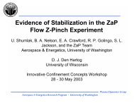
construct configuration tracking controls for our classesof second-order systems. In Section 5, we discuss ourresults and some directions for continued research.Recall that the equations describing an underactuatedmechanical system can be written asM(x)ẍ + C(x, ẋ) + P (x) = B(x)u, (2)where x ∈ R n , u ∈ R m , B(x) = [ ˜B T (x), 0 T ] T and˜B(x) ∈ R m×m . One may solve these equations for ẍand use feedback to getẍ =m∑g i (x)u i + h(x, ẋ) = G(x)u + h(x, ẋ).i=1In addition to these mechanical systems, one has twoadditional more or less natural classes of systems obtainedby cascading a drift-free nonholonomic system(1) with a set of integrators. These three classes canbe summarized as{ ˙ξ = u(CI)ẋ = ∑ mi=1 g i(x)ξ i{ ∑ m ˙ξ =(CS)i=1 g i(ξ)u iẋ = ξ(CM){ ˙ξ =∑ mi=1 g i(x)u i + h(x, ξ)ẋ = ξrespectively termed cascade input (CI), cascade state(CS), and cascade mechanical (CM). We could generalizefurther by replacing the set of integrators witha full linear system, but will leave this setting for anappropriate lengthier discussion. In the following workwe will focus on the subclass of (CM) systems whereh(x, ẋ) = 0. In general this disallows the presence ofCoriolis, centrifugal and gravity forces as well as dampingand Coulomb friction. However, in some circumstancessuch as systems with a triangular structure, thisassumption can be met after the elimination of termsvia feedback and/or state space transformations.As an example, by extending the nonholonomic integratorẋ 1 = u 1 , ẋ 2 = u 2 , ẋ 3 = x 1 u 2 − x 2 u 1 to (CI)-(CM),we have(nhi − ci)(nhi − cs)(nhi − cm)X X 2 2X 1nonholonomic integrator ż⎧1 = v 1 , ż 2 = v 2 , ż 3 =⎨ ẍ 1 = u 1z 1 v 2 − z 2 v 1 . Thus we can design controls for the nonholonomicintegrator and apply them to the kinematicẍ 2 = u 2⎩ẋ 3 = x 1 ẋ 2 − x 2 ẋ 1mobile robot. We will use this example to demonstrateconfiguration tracking with (CM) systems.⎧⎨ ẍ 1 = u 13 Controllabilityẍ 2 = u 2⎩ẍ 3 = ẋ 1 u 2 − ẋ 2 u 1The systems we are considering here fall into the class⎧of control affine nonlinear systems with drift:⎨ ẍ 1 = u 1m∑ẍ 2 = u 2⎩ẋ = f(x) + g i (x)u i (6)ẍ 3 = x 1 u 2 − x 2 u 1An important point to note in the mechanical extensionof the nonholonomic integrator is that the third stateis integrable. Namely x 1 u 2 − x 2 u 1 = d dt (x 1ẋ 2 − x 2 ẋ 1 ).2 ModelsThis system then reduces to the form (CI) and is effectivelykinematic. Conditions for the equivalence ofa given mechanical system to a kinematic structure arediscussed in [14] and feedback transformations to convertmechanical systems to (CI) form are shown in [8].To demonstrate a controllable (CM) system, considerthe vehicle in Fig. 1a with unit axle length and wheelradius. A kinematic description of the position andF x 1Fx2X 1(a)(b)Figure 1: Differential drive two wheel vehicle (a), andunderactuated planar link (b).orientation of the axle center is given byẋ 1 = cos(θ)u 1 , ẋ 2 = sin(θ)u 1 , ˙θ = u2 . (3)Now consider the equations of motion for the center ofmass of an underactuated link in the plane (Fig. 1b).Arbitrary forces can be applied to a free joint at oneend of the link, but no torques may be applied. Onecan show (e.g. [1]) that the equations of motion for thissystem can be reduced toẍ 1 = cos(θ)u 1 , ẍ 2 = sin(θ)u 1 , ¨θ = u2which is a mechanical extension of (3). With the statespace transformationz 1 = x 1 cos(θ) + x 2 sin(θ)z 2 = θ (4)z 3 = 2(x 1 sin(θ) − x 2 cos(θ)) − θ(x 1 cos(θ) + x 2 sin(θ))and the control space transformationv 1 = r 1 u 1 − r 2 u 2 (x 1 sin(θ) − x 2 cos(θ))v 2 = r 2 u 2 (5)the system equations (3) can be converted into thei=1

where x ∈ M, M is a smooth n-dimensional manifoldand u ∈ R m . For a complete treatment of nonlinearaccessibility and controllability, the reader is referredto [12, 22]. We will state the relevant definitions herefor reference.Definition 3.1 The system (6) is controllable if forany two equilibrium points p, q ∈ M, there exists a finitetime T and control functions u : [0, T ] → R m suchthat x(0) = p and x(T ) = q. The system (6) is smalltime locally controllable (STLC) if for every for equilibriumpoint p ∈ M and T > 0, the set reachable fromp in time T contains p in its interior.From [23], we have the following result for (CI) systems.Proposition 3.2 (Sussmann [23]) Given any driftfreecontrollable nonlinear system (1), the cascade inputsystem (CI) is both controllable and STLC.Controllability results for (CS) and (CM) systems arenot as strong as for (CI) systems, however, each of theseclasses is fully accessible. Under certain conditions,STLC can also be shown.Proposition 3.3 Given any drift-free controllablenonlinear system (1), the cascade state system (CS)is fully accessible.Proof: In order for a nonlinear system to be accessible,we simply need to show that the Lie Algebra RankCondition (LARC) is satisfied at all p ∈ M. Definez = [ξ T , x T ] T , and rewrite the overall system equationsin the form[ ]0ż = + ∑ [ ]gi (ξ)uξ0 i = ˜f(z) + ∑ ˜g i (z)u i .iiStraightforward calculations show that[ ][gj (ξ), g[˜g j , ˜g i ] =i (ξ)]0[ ][gk (ξ), [g[˜g k , [˜g j , ˜g i ]] =j (ξ), g i (ξ)]]0.[˜f, ˜gi][˜f, [˜gj , ˜g i ]]==.[[0g i (ξ)]0[g j (ξ), g i (ξ)]As long as the original drift-free system is controllable,these vector fields will span R n × R n at all points. ✷]Proposition 3.4 Any cascade state system (CS) fullyaccessible with Lie brackets of order no more than fouris STLC.Proof: For i = 1, . . . , m let δ i be the number of occurrencesof the vector fields g i and δ 0 be the numberof occurrences of the vector field f in a Lie bracket B.From [22], we refer to a bracket B as bad if δ 0 is odd andeach δ i is even and good otherwise. A sufficient conditionfor a system to be STLC is that all bad brackets atan equilibrium point p are linear combinations of goodbrackets of lower degree. From the previous proposition,we see immediately that the only bad bracketsof degree less than four are those of degree three withi = j and δ 0 = 1 or 3. However, in those cases the badbrackets are identically zero ([g i , g i ] ≡ 0 and f(p) ≡ 0).✷Proposition 3.5 (Reyhanoglu et al. [20]) A cascademechanical system (CM) is fully accessible if eachnonlinear state equation is nonintegrable.Proposition 3.6 (Reyhanoglu et al. [20]) If a(CM) system is fully accessible with the brackets{g i , [f, g i ], [g j , [f, g i ]], [f, [g j , [f, g i ]]]}, then it is STLCfrom all equilibrium points.While we do not have a general controllability statementfor (CS) and (CM) systems, we will see in the nextsection that when the drift-free portion of the systemis controllable, we can always perform configurationtracking.4 Trajectory TrackingAs shown in [5, 16, 17, 18], amplitude-modulated sinusoidalcontrols can be used to generate motion inthe constrained states of a drift-free nonholonomic system.We refer the reader to the references for detailsand state the basic result here. For readability, we willsometimes suppress explicit time dependence.Proposition 4.1 Given the twice differentiable functionsx d (t) ∈ R n and a controllable, drift-free nonholonomicsystem (1), there exist ω-parameterized controlsof the form2(n−m)∑u (ω)i (t) = γ i (x d , ẋ d ) + α ij (x d , ẋ d ) sin(λ ij ωt)2(n−m)∑+j=1j=1β ij (x d , ẋ d ) cos(µ ij ωt) (7)such that, for matched initial conditions and with respectto an L 2 norm, lim ω→∞ x (ω) (t) = x d (t).

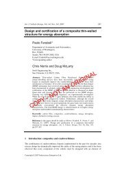
Note that for each state x i such that ẋ i = u i , we willhave γ i = ẋ d,i .Example: Consider the nonholonomic integrator ẋ 1 =u 1 , ẋ 2 = u 2 , ẋ 3 = x 1 u 2 − x 2 u 1 and the controlsu 1 (t) = ẋ d,1 + √ ω sin(ωt)u 2 (t) = ẋ d,2 − √ ωβ(t) cos(ωt) (8)where β(t) = ẋ d,3 −x d,1 ẋ d,2 +x d,2 ẋ d,1 . Integrating eachof the controls once by parts and assuming matchedinitial conditions leads tox 1 (t) = x d,1 (t) − 1 √ ωcos(ωt)x 2 (t) = x d,2 (t) − 1 √ ωβ(t) sin(ωt)−√ 1 ∫ td(β(τ)) sin(ωτ)dτ.ω dτThe third state then evolves according to( )1x 3 (t) = x d,3 (t) − √ω ẋ d,1 + sin(ωt) ·0∫ t0d(β(τ)) sin(ωτ)dτdτTo eliminate the integral terms, we use a version of theRiemann-Lebesgue lemma:Lemma 4.2 (Riemann-Lebesgue [9]) Let f be ofbounded variation on [a, b] and let φ ∈ [0, 2π]. Thenlim ω→∞∫ ba f(t) cos(ωt + φ)dt = o ( 1ω).In the limit as ω becomes large, we have x (ω) (t) ≈x d (t).Now we will show how a result of this form for a driftfreesystem can be extended to our classes of secondordersystems to produce configuration tracking.Corollary 4.3 ((CI) Configuration Tracking)Given a controllable (CI) system, three times differentiablefunctions x d (t) and approximate trackingcontrols (7) for the system ẋ = G(x)u, definev (ω)i (t) = d dt γ i(x d , ẋ d )2(n−m)∑+j=12(n−m)∑−j=1λ ij ωα ij (x d , ẋ d ) cos(λ ij ωt)µ ij ωβ ij (x d , ẋ d ) sin(µ ij ωt). (9)Denote by [ξ, x] (ω) the solution to (CI) for the controlsv (ω) . Then for matched initial conditions and with respectto the L 2 norm, lim ω→∞ x (ω) (t) = x d (t).2x 1 0−20.5x 2 0−0.52x 3 0−20 10 20 30 40 50tFigure 2: Tracking for (nhi-ci) dynamic system.Proof: Integrating the inputs once by parts givesξ (ω)i (t) = γ(x d (t), ẋ d (t)) − γ(x d (0), ẋ d (0)) + ξ (ω)i (0)2(n−m)∑+−j=12(n−m)∑j=12(n−m)∑+−j=12(n−m)∑j=1α ij (x d , ẋ d ) sin(λ ij ωτ)| t 0∫ t0ddτ (α ij(x d , ẋ d )) sin(λ ij ωτ)dτβ ij (x d , ẋ d ) cos(µ ij ωτ)| t 0∫ t0ddτ (β ij(x d , ẋ d )) cos(µ ij ωτ)dτAssuming matched initial conditions and applying theRiemann-Lebesgue lemma gives2(n−m)∑ξ (ω)i (t) = γ(x d , ẋ d ) + α ij (x d , ẋ d ) sin(λ ij ωt)2(n−m)∑+j=1j=1( ) 1β(x d , ẋ d ) cos(µ ij ωt) + oωIn the limit as ω becomes large, we have recovered thecontrols (7) which by assumption gives the result. ✷An example of tracking using these controls with thesystem (nhi-ci) is shown in Fig. 2 for ω = 25. Theplot shows the actual position trajectories as solid linesoverlaid on dashed lines representing the desired trajectories.The higher order terms that we discarded whileconstructing our control law will cause the introductionof a constant error in the matched initial conditions atthe velocity level. As ω becomes large, the error willdecrease.Corollary 4.4 ((CS) Configuration Tracking)Given a controllable (CS) system, three times differentiablefunctions x d (t) and approximate tracking

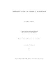
2x 1 0−25x 2 0−52x 3 0−20 10 20 30 40 50tFigure 3: Tracking for (nhi-cs) dynamic system.controls (7) for the system ˙ξ = G(ξ)u, define2(n−m)∑v (ω)i (t) = γ(ẋ, ẍ d ) + α ij (ẋ d , ẍ d ) sin(λ ij ωt)2(n−m)∑+j=1j=1β ij (ẋ d , ẍ d ) cos(µ ij ωt). (10)Denote by [ξ, x] (ω) the solution to (CM) for the controlsv (ω) . Then for matched initial conditions and with respectto the L 2 norm, lim ω→∞ x (ω) (t) = x d (t).Proof: Directly using the result from Prop. 4.1 gives( ) 1ξ (ω) (t) = ẋ d (t) + o .ωOne additional integration and the assumption x(0) =ẋ d (0) gives( ) 1x (ω) (t) = x d (t) + oωand the result follows in the limit ω → ∞.An example of tracking with these controls for the system(nhi-cs) is shown in Fig. 3 with a frequency ofω = 10. The dashed line represents the desired signals,and the solid line shows the system response.To demonstrate how trajectory tracking for drift-freesystems can be extended to (CM) systems, we will restrictour attention to the classẋ =[ẋl] [=ẋ nl✷u l˜G(x l )u nl]= G(x l )u (11)where x l , u l ∈ R p , p < m, x nl ∈ R n−p , u nl ∈ R m−p ,and the subscripts l and nl refer respectively to statesthat are linear and nonlinear. Results for the generalcase can be stated, but the corresponding proofs arebeyond the scope of this text.Corollary 4.5 ((CM) Configuration Tracking)Given a controllable (CM) system with G(x)v of theform (11), three times differentiable functions x d (t)and approximate tracking controls (7) for the system(11), define2(n−m)∑v (ω)l,i= ẍ d,l,i + λ ij ωα ij (z d , ż d ) cos(λ ij ωt)2(n−m)∑−j=1j=1µ ij ωβ ij (z d , ż d ) sin(µ ij ωt)2(n−m)∑v (ω)nl,k= γ k (z d , ż d ) + α kj (z d , ż d ) sin(λ kj ωt)2(n−m)∑+j=1j=1β kj (z d , ż d ) cos(µ kj ωt) (12)where i = 1, . . . , p, k = p + 1, . . . , m, and z d =[x d,l , ẋ d,nl ]. Denote by [ξ, x] (ω) the solution to (CM) forthe controls v (ω) . For matched initial conditions andwith respect to the L 2 norm, lim ω→∞ x (ω) (t) = x d (t).Proof: Integrate the controls v (ω)l,itwice by parts andassume matching initial conditions to get2(n−m)ξ (ω)l,i (t) = ẋ ∑d,i + α ij (z d , ż d ) sin(λ ij ωt)2(n−m)∑+j=1j=1( ) 1β ij (z d , ż d ) cos(µ ij ωt) + oω2(n−m)x (ω)l,i (t) = x ∑ 1d,i −λ ij ω α ij(z d , ż d ) cos(λ ij ωt)j=12(n−m)∑( )11+µ ij ω β ij(z d , ż d ) sin(µ ij ωt) + oωj=1which is exactly the result obtained by integrating theportion of controls (7) corresponding to u l in (11).When z d = [x d,l , x d,nl ] in v (ω)nl,k, we recover the controls(7) corresponding to u nl , and G(x l )v nl = ẋ d,nl + o ( )1ω .In order to have the desired result of G(x l )v nl =ẍ d,nl + o ( 1ω), we simply choose zd = [x d,l , ẋ d,nl ]. Twofinal integrations assuming matched initial conditionsgives the stated result.✷The underactuated link in the plane (4) is a (CM) systemof the type in Cor. 4.5. Using the controls (8) with(5), the drift-free system (3) can track [x 1d , x 2d , θ d ]withu 1 = γ(t) + ω 1 2 sin(ωt) − ω12 m(t)η(t) cos(ωt)u 2 = ˙θ d (t) − ω 1 2 m(t) cos(ωt)

2x 1 0−20220 40 60 80 100x 2 0−20220 40 60 80 100x 3 0−20 20 40 60 80 100Figure 4: Tracking for underactuated planar link.where γ = ż 1 + ż 2 η, m = ż 3 − (ż 2 z 1 − ż 1 z 2 ), η =x d,1 sin(θ d ) − x d,2 cos(θ d ), z 1 = x d,1 cos(θ) + x d,2 sin(θ),z 3 = 2η − θ d z 1 . Modifying the kinematic controls asshown in the corollary gives usv 1 = γ(t) + ω 1 2 sin(ωt) + ω12 m(t)γ(t) cos(ωt)v 2 = ¨θ d (t) + ω 1 2 m(t) sin(ωt)where we make the substitutions η = ẋ d,1 sin(θ d ) −ẋ d,2 cos(θ d ) and z 1 = ẋ d,1 cos(θ) + ẋ d,2 sin(θ). An exampleof these controls for ω = 10 is shown in Fig. 4.5 ConclusionGiven the reduction of a mechanical system to the cascadeof a drift-free nonholonomic system and a set ofintegrators, we have shown for some such classes howamplitude-modulated sinusoidal controls can be constructedto achieve configuration tracking. The generalcase of (CM) systems was not presented here, butwill be handled in subsequent work. Finally, the type ofcontrols presented here do not take into account boundson actuator amplitude or frequency. As the frequencyis increased to produce greater tracking accuracy, physicalactuators will quickly reach performance limits.Simultaneously handling limits on tracking errors andlimits on actuators is a topic of current research.References[1] H. Arai, K. Tanie, and N. Shiroma. Nonholonomiccontrol of a three-DOF planar underactuated manipulator.IEEE Trans. Rob. Aut., 14(5):681–695, 1998.[2] A.M. Bloch and P.E. Crouch. Nonholonomic controlsystems on Riemannian manifolds. SIAM J. Contr. Optim.,33(1):126–48, Jan. 1995.[3] A.M. Bloch, M. Reyhanoglu, and N.H. McClamroch.Control and stabilization of nonholonomic dynamic systems.IEEE Trans. Aut. Contr., 37(11):1746–57, Nov. 1992.[4] R.W. Brockett. Asymptotic stability and feedbackstabilization. In R. W. Brockett, R. S. Millman, and H. J.Sussmann, editors, Differential Geometric Control Theory,pages 181–91. Birkhäuser, 1983.[5] R.W. Brockett. Characteristic phenomena and modelproblems in nonlinear control. In Proc. IFAC Congress,pages 135–40, 1996.[6] F. Bullo, N.E. Leonard, and A.D. Lewis. Controllabilityand motion algorithms for underactuated Lagrangiansystems on Lie groups. IEEE Trans. Aut. Contr.,45(8):1437–54, 2000.[7] F. Bullo and K.M. Lynch. Kinematic controllabilityand decoupled trajectory planning for underactuatedmechanical systems. In Proc. IEEE Int. Conf. Rob. Aut.,pages 3300–7, 2001.[8] G. Campion, B. D’Andrea-Novel, and G. Bastin. AdvancedRobot Control, chapter Controllability and statefeedback stabilizability of nonholonomic mechanical systems,pages 106–24. 1991.[9] J.B. Conway. A Course in Functional Analysis.Springer-Verlag, 1990.[10] C. Canudas de Wit and O.J. Sordalen. Exponentialstabilization of mobile robots with nonholonomic constraints.IEEE Trans. Aut. Contr., 37(11):1791–7, Nov.1992.[11] O. Egeland, M. Dalsmo, and O.J. Sordalen. Feedbackcontrol of a nonholonomic underwater vehicle with a constantdesired configuration. Int. J. Robot. Res., 15(1):24–35,Feb. 1996.[12] A. Isidori. Nonlinear Control Systems. Springer-Verlag, Berlin, Germany, 2 edition, 1985.[13] N.E. Leonard. Periodic forcing, dynamics and controlof underactuated spacecraft and underwater vehicles. InProc. 34th IEEE Conf. Dec. Cont., pages 1131–6, 1995.[14] A.D. Lewis. When is a mechanical control systemkinematic? In Proc. 38th IEEE Conf. Dec. Cont., pages1162–7, 1999.[15] A.D. Lewis and R.M. Murray. Configuration controllabilityof simple mechanical control systems. SIAM J.Contr. Optim., 35(3):766–90, 1997.[16] W. Liu. An approximation algorithm for nonholonomicsystems. SIAM J. Contr. Optim., 35(4):1328–65,Jul. 1997.[17] K.A. Morgansen and R.W. Brockett. Trajectorytracking from approximate inversion for driftless nonholonomicsystems. 2001.[18] R.M. Murray and S. Sastry. Nonholonomic motionplanning: Steering using sinusoids. IEEE Trans. Aut.Contr., 38(5):700–16, May 1993.[19] Ju.I. Neimark and N.A. Fufaev. Dynamics of NonholonomicSystems. American Mathematical Society, Providence,RI, 1972.[20] M. Reyhanoglu, A. van der Schaft, N.H. McClamroch,and I. Kolmanovsky. Dynamics and control of a classof underactuated mechanical systems. IEEE Trans. Aut.Contr., 44(9):1663–71, Sep. 1999.[21] O.J. Sordalen and O. Egeland. Exponential stabilizationof nonholonomic chained systems. IEEE Trans. Aut.Contr., 40(1):35–49, Jan. 1995.[22] H.J. Sussmann. A general theorem on local controllability.SIAM J. Contr. Optim., 25(1):158–94, Jan. 1987.[23] H.J. Sussmann. Local controllability and motionplanning for some classes of systems with drift. In Proc.30th IEEE Conf. Dec. Contr., pages 1110–4, 1991.