Object based contour detection by using Graph-cut on Stereo image

label assingning L p {1,2,3}. This labeling means segment
image that we want[2][4].
We can formulate a standard form of the energy function
to solve this pixel labeling problem[1][2][3][4][5].
The form of energy function is
E( f ) E ( f ) E ( f )
E data (f) and E smooth (f) can be also represented as follows
E ( f )
This function includes a variety of different concept such
as first-order Markov Random Fields. D p (f p ) is a data
penalty function and it means that how well assign a label
f p to a pixel p given the observed data. V p,q (f p , f q )
penalizing between neighboring pixels p, qN is spatial
smoothness term. N is the set of neighboring pixels of
left image. V can be separated from metric and
semi-metric. For any labels , , L
V(, ) = 0 = (2)
V(, ) = V(, ) (3)
V(, ) V(, ) + V(, ) (4)
If V satisfy (2),(3) and (4), V is metric on the space of
Label L. Also V is called a semi-metric if it satisfies only
(2),(3)[2]. We can specify this equation <strong>by</strong> potts model as
follows.
E ( f )
pP
pL
data
D
D
p
p
( f
( f
p
p
)
)
smooth
V
p.
qN
V
p . qN
p , q
( f
T
, f
Here T() is 1 if its argument is true and 0 otherwise[1][3].
Our goal is to find labeling f for local
minimum to minimize energy function(1). We can also
use -expansion move algorithm to generate labeling f.
This is a strong move allowing many pixels to change
their labels to simultaneously. Given a label ,
-expansion is a move from a partition P(labeling f) to a
new partition P’ if P P ’ and P l ’ P l for any label l
[2].
In pixel labeling problem, We have to find f that minimize
energy function. To solve this problem, We can use
graph <strong>cut</strong> method.
p
f
p , q
(
p q
)
q
)
f
(1)
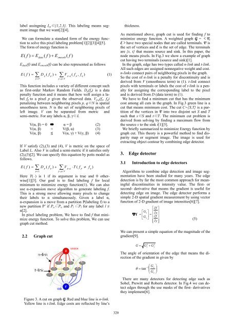
thickness.
As mentioned above, graph <strong>cut</strong> is used for finding f to
minimize energy function. A weighted graph G = V,
Ehave two special nodes that are called terminals. V is
the set of vertices and E is the set of edge. The terminals
are {s, t} that means source and sink. In this paper, the
node means pixels. In Fig.3 we show a example of graph
<strong>cut</strong> having two terminals (source and sink)[1].
In the graph, edge has two types called n-link and t-link.
All such edges are assigned nonnegative weight and cost.
n-links connect pairs of neighboring pixels in the graph.
So the cost of n-link is a penalty for discontinuity and is
derived from V (smoothness term) in (1). t-link connect
pixels with terminals or labels the cost of t-link is a penalty
for assigning the corresponding label to the pixel
and is derived from D (data term) in (1).
We have to find a minimum <strong>cut</strong> that has the minimum
cost among all <strong>cut</strong>s in the graph. In Fig.3 green line is a
<strong>cut</strong> that means minimum cost. The <strong>cut</strong> C={S,T} is a partition
of the vertices in V into two disjoint set S and T
such that s S and tT. The minimum <strong>cut</strong> problem is
derived from solving <strong>by</strong> finding a maximum flow from
the source s to the sink t[1][5].
We briefly summarized to minimize Energy function <strong>by</strong>
graph <strong>cut</strong>. This theory is a powerful method to find disparity
map or segment image. The image is used for
extracting object <strong>contour</strong> <strong>by</strong> combining edge detector.
3. Edge detector
3.1 Introduction to edge detectors
Algorithms to combine edge <strong>detection</strong> and image segmentation
have been studied for many years. The edge
<strong>detection</strong> is <strong>by</strong> far the most common approach for meaningful
discontinuities in intensity value. The first- or
second- derivative that means the gradient is useful for
detecting edge on image. The edge detector performs a
simple 2-D spatial gradient measurement <strong>by</strong> <strong>using</strong> vector
function of 2-D gradient of image intensities[6][7].
f
f
f x
Gy
y
(5)
G x
2
2.2 <strong>Graph</strong> <strong>cut</strong>
We can present a simple equation of the magnitude of the
gradient[9].
G
2
G x
G y
The angle of orientation of the edge that means the direction
of the gradient in given <strong>by</strong>
Figure 3. A <strong>cut</strong> on graph G. Red and blue line is n-link.
Yellow line is t-link. Edge costs are reflected <strong>by</strong> line’s
tan
1
G
G
y
x
There are many detectors for detecting edge such as
Sobel, Prewitt and Roberts detector. In Fig.4 we can detect
edges through the use masks of the first- derivatives
they implement[6].
320