Object based contour detection by using Graph-cut on Stereo image

8-23
MVA2007 IAPR Conference on Machine Vision Applications, May 16-18, 2007, Tokyo, JAPAN
<strong>Object</strong> <strong>based</strong> <strong>contour</strong> <strong>detection</strong> <strong>by</strong> <strong>using</strong> <strong>Graph</strong>-<strong>cut</strong> on Stereo image
Taehoon Kang 1 , Jaeseung Yu 1 , Jangseok Oh 1 , Yunhwan Seol 1 , Kwanghee Choi 1 , Mingi Kim 1*
1 Korea Univ., Department ofElectronics and Information Engineering,
Anam-Dong, Seongbuk-Gu, Seoul 136-701, Korea
{dreamth, yu1227, dueleldi, yhseol, wastedtime, mgkim}@korea.ac.kr
Abstract
In the last few years, computer vision and image processing
techniques have been developed to solve many
problems. One of them, graph <strong>cut</strong> method is powerful
optimization technique for minimizing energy function.
And as you know, many edge detectors are already advanced.
Edge detector is widely used in computer vision
to find object boundaries in images. But traditional edge
detectors detect all edges that we don’t want. Because we
want to detect object <strong>contour</strong>, we propose that graph <strong>cut</strong>
method and edge detector have to combine each other. In
this paper, we describe method minimizing energy function
via graph <strong>cut</strong>s and traditional edge detectors and
show our result images.
1. Introduction
One of the most important techniques in computer vision
is to extract object <strong>contour</strong> in images. In recent,
energy minimization techniques <strong>based</strong> on graph <strong>cut</strong>s are
used for applications such as image segmentation, restoration,
stereo, object recognition and some others
[1][2][3][4][5]. This methods gives very strong experimental
results. To solve our problem, we used standard
stereo geometry such as shown in Fig.1, where a pair of
point M 1 M 2 called corresponding point.
applications, such as image segmentation, region separation,
and recognition use edge <strong>detection</strong> as preprocessing
stage for feature extraction[6][8]. The edge means a
sudden change in image intensity so that the edge may
not guaranty the object boundary. With the segment image
<strong>by</strong> graph <strong>cut</strong>s, the Canny edge detector[7] classifies a
pixel as an edge if the gradient magnitude of pixel is
larger than those of pixels at both its sides in the direction
of maximum intensity change. In general images,
edge detector search all edges that we don’t want. Because
of this reason, we will combine graph <strong>cut</strong>s method
and the Canny edge detector to find object <strong>contour</strong> that
we want.
The most important algorithm described in this paper is
<strong>based</strong> on energy minimization because we have to find
out a correct segmented image[1][2]. In this method, our
focus is to find global minimum of energy function
where it is NP-hard to compute global minimum[2]. We
then describe two algorithms <strong>based</strong> on graph <strong>cut</strong>s,
namely expansion moves and swap moves[2][4] computes
efficiently a local minimum of energy function. We
present only expansion moves that used in our algorithms
for energy minimization.
This paper is organized as follows. In section 2 we begin
with overview of energy minimization algorithms via
graph <strong>cut</strong>s. We review some different edge detector and
the canny edge detector that technique enhanced is introduced
in section 3. We show the experimental result
images in section 4 and discuss conclusion in section 5.
2. Energy minimization <strong>by</strong> graph <strong>cut</strong>s
2.1 Energy function
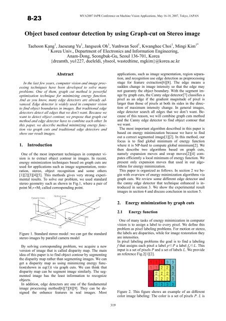
Figure 1. Standard stereo model :we can get the standard
stereo images <strong>by</strong> parallel camera model
By solving corresponding problem, we acquire a new
version of image that is called disparity map. The main
idea of this paper is to find object <strong>contour</strong> <strong>by</strong> segmenting
the disparity map rather than segmenting images. We can
get a disparity map as <strong>using</strong> minimizing energy function(shown
in eq(1)) via graph <strong>cut</strong>s. We can think that
disparity map can be segment image similarly. The segmented
image has the least information to recognize
objects.
In addition, edge detectors are one of the fundamental
image processing method[6][7][8][9]. They can be designed
the enhance features in real images. Most
One of many tasks of energy minimization in computer
vision is to assign a label to every pixel. We define this
problem as pixel labeling problems. For motion or stereo,
the labels are disparities, while for image restoration they
are intensities.
In pixel labeling problems the goal is to find a labeling
f that assigns each pixel a label pP a label f p L. This
input is a set of pixels P and a set of labels L. We provide
an reference Fig.2[1][2].
Figure 2. This figure shows an example of an different
color image labeling: The color is a set of pixels P. L is
319

label assingning L p {1,2,3}. This labeling means segment
image that we want[2][4].
We can formulate a standard form of the energy function
to solve this pixel labeling problem[1][2][3][4][5].
The form of energy function is
E( f ) E ( f ) E ( f )
E data (f) and E smooth (f) can be also represented as follows
E ( f )
This function includes a variety of different concept such
as first-order Markov Random Fields. D p (f p ) is a data
penalty function and it means that how well assign a label
f p to a pixel p given the observed data. V p,q (f p , f q )
penalizing between neighboring pixels p, qN is spatial
smoothness term. N is the set of neighboring pixels of
left image. V can be separated from metric and
semi-metric. For any labels , , L
V(, ) = 0 = (2)
V(, ) = V(, ) (3)
V(, ) V(, ) + V(, ) (4)
If V satisfy (2),(3) and (4), V is metric on the space of
Label L. Also V is called a semi-metric if it satisfies only
(2),(3)[2]. We can specify this equation <strong>by</strong> potts model as
follows.
E ( f )
pP
pL
data
D
D
p
p
( f
( f
p
p
)
)
smooth
V
p.
qN
V
p . qN
p , q
( f
T
, f
Here T() is 1 if its argument is true and 0 otherwise[1][3].
Our goal is to find labeling f for local
minimum to minimize energy function(1). We can also
use -expansion move algorithm to generate labeling f.
This is a strong move allowing many pixels to change
their labels to simultaneously. Given a label ,
-expansion is a move from a partition P(labeling f) to a
new partition P’ if P P ’ and P l ’ P l for any label l
[2].
In pixel labeling problem, We have to find f that minimize
energy function. To solve this problem, We can use
graph <strong>cut</strong> method.
p
f
p , q
(
p q
)
q
)
f
(1)
thickness.
As mentioned above, graph <strong>cut</strong> is used for finding f to
minimize energy function. A weighted graph G = V,
Ehave two special nodes that are called terminals. V is
the set of vertices and E is the set of edge. The terminals
are {s, t} that means source and sink. In this paper, the
node means pixels. In Fig.3 we show a example of graph
<strong>cut</strong> having two terminals (source and sink)[1].
In the graph, edge has two types called n-link and t-link.
All such edges are assigned nonnegative weight and cost.
n-links connect pairs of neighboring pixels in the graph.
So the cost of n-link is a penalty for discontinuity and is
derived from V (smoothness term) in (1). t-link connect
pixels with terminals or labels the cost of t-link is a penalty
for assigning the corresponding label to the pixel
and is derived from D (data term) in (1).
We have to find a minimum <strong>cut</strong> that has the minimum
cost among all <strong>cut</strong>s in the graph. In Fig.3 green line is a
<strong>cut</strong> that means minimum cost. The <strong>cut</strong> C={S,T} is a partition
of the vertices in V into two disjoint set S and T
such that s S and tT. The minimum <strong>cut</strong> problem is
derived from solving <strong>by</strong> finding a maximum flow from
the source s to the sink t[1][5].
We briefly summarized to minimize Energy function <strong>by</strong>
graph <strong>cut</strong>. This theory is a powerful method to find disparity
map or segment image. The image is used for
extracting object <strong>contour</strong> <strong>by</strong> combining edge detector.
3. Edge detector
3.1 Introduction to edge detectors
Algorithms to combine edge <strong>detection</strong> and image segmentation
have been studied for many years. The edge
<strong>detection</strong> is <strong>by</strong> far the most common approach for meaningful
discontinuities in intensity value. The first- or
second- derivative that means the gradient is useful for
detecting edge on image. The edge detector performs a
simple 2-D spatial gradient measurement <strong>by</strong> <strong>using</strong> vector
function of 2-D gradient of image intensities[6][7].
f
f
f x
Gy
y
(5)
G x
2
2.2 <strong>Graph</strong> <strong>cut</strong>
We can present a simple equation of the magnitude of the
gradient[9].
G
2
G x
G y
The angle of orientation of the edge that means the direction
of the gradient in given <strong>by</strong>
Figure 3. A <strong>cut</strong> on graph G. Red and blue line is n-link.
Yellow line is t-link. Edge costs are reflected <strong>by</strong> line’s
tan
1
G
G
y
x
There are many detectors for detecting edge such as
Sobel, Prewitt and Roberts detector. In Fig.4 we can detect
edges through the use masks of the first- derivatives
they implement[6].
320

Prewitt mask
-1 -1 -1 -1 0 1
0 0 0 -1 0 1
1 1 1 -1 0 1
G x
G y
Sobel mask
-1 -2 -1 -1 0 1
0 0 0 -2 0 2
1 2 1 -1 0 1
G x
G y
Roberts mask
-1 0 0 -1
0 1 1 0
G x
G y
Figure 4. Masks of some edge detector. G x and G y are the
first derivatives of gradient vector.
3.2 Canny edge detector
The Canny edge detector developed <strong>by</strong> John Canny [7]
is the optimal detector used around the world. This edge
detector is <strong>based</strong> on detecting at the zero-crossing of the
second directional derivative of the smoothed image. The
procedure of the Canny edge detector was as follows [6]:
1. We can use an appropriate 2-D Gaussian filter
to make smoothed image.
2. In smoothed image we have to compute the
gradient direction and magnitude at each point.
An edge point is defined that strength of the
point is locally maximum in the direction of the
gradient.
3. Perform non-maximal suppression. The edge
point determined above rise to ridges in the
gradient magnitude image. Tracking the top of
the ridges and set to zero all pixels that are not
on the ridge top to make a thin line in the output
image.
4. The ridge pixels are thresholded <strong>by</strong> <strong>using</strong> T1
and T2 with T1

We apply the Canny edge detector to output image <strong>by</strong>
graph <strong>cut</strong>s in order to find object boundary. Fig.6 shows
the difference of the result in the same condition of parameter.
In this Fig.6 we use the same parameter of
T1=0.05 and T2=0.1. As mentioned above the T1, T2
means threshold values. The parameters was obtained <strong>by</strong>
repeated experiments and can adopt the optimized results.
The left images have edges of all objects. We don’t need
all edges when we detect or track objects. Hence, we
readjust parameters, T1 and T2 to show the result of object
boundary we want.
edge detector performs good results for finding object
boundary. Our results show the general boundary of the
objects. However, the <strong>contour</strong> extracted <strong>by</strong> our segmented
image of Fig.6 is not matched with the exact
boundary. In addition, our final goal is to extract
boundaries of each object we want to find. For instance,
if we want to find only the boundary of camera in Tsukuba
image, our algorithm is limited. To improve the
more accurate boundary, our future works will use snake
algorithms of active <strong>contour</strong> model[10]. In snake algorithm,
we can consider the boundaries of our results as
initial points. We believe that our algorithm will get a
powerful result if active <strong>contour</strong> algorithm is inserted.
Acknowledgements
(a)
(c)
(b)
Figure 7. The developed result of the Canny edge detector.
It is the more specified object <strong>contour</strong> that we want.
The main results of our experiment are illustrated in
Fig.7. The Canny edge detector computes a gradient direction
and magnitude for each pixel of the segmented
image. We tried several times to find an appropriate
boundary of object. We can compare our results of the
right images of Fig.6 and the results of Fig.7. Fig.7
shows the better performance than Fig.6. The resetted
values of parameter are T1=0.2 and T2=0.7 in (a),
T1=0.05 and T2=0.3 in (b). In (c) the parameter values
are T1 = 0.1 and T2 = 0.511. The algorithm is powerful
enough to detect object <strong>contour</strong> in images as changing
parameter values.
5. Conclusions
In this paper, We assume the acquired images satisfy
the standard stereo geometry. However, the image we
acquire may not satisfy the geometry. Thus we are preparing
the image rectification stage. We have shown that
combining graph <strong>cut</strong>s algorithm and edge <strong>detection</strong> are
useful algorithms for detecting object <strong>contour</strong>. Our approach
is <strong>based</strong> on the constraint that the images are
standard stereo. We suggest that the use of the Canny
This research was supported <strong>by</strong> a grant from Strategic
National R&D Program of Ministry of Commerce, Industry
and Energy.
References
[1] Boykov, Y., Kolmogorov, V., “An Experimental Comparison
of Min-Cut/Max-Flow Algorithms for Energy
Minimization in Vision”, In IEEE Transactions on PAMI,
Vol. 26, No. 9, pp. 1124-1137, 2004
[2] Boykov, Y., Veksler, O.Zabih, R., “Fast Approximate Energy
Minimization via <strong>Graph</strong> Cuts”, Proc. IEEE Trans.
Pattern Analysis and Machine Intelligence, vol. 23, no. 11,
pp. 1222-123, 2001
[3] V. Kolmogorov and R. Zabih, “Computing Visual Correspondence
with Occlusions via <strong>Graph</strong> Cuts,” Proc. Int'l
Conf. Computer Vision, vol. 2, pp. 508-515, 2001.
[4] Olga Veksler. “Effcient <strong>Graph</strong>-<strong>based</strong> Energy Minimization
Methods in Computer Vision.” PhD thesis, Cornell University,
July 1999.
[5] V. Kolmogorov and R. Zabih. “What energy functions can
be minimized via graph <strong>cut</strong>s” IEEE Transactions on Pattern
Analysis and Machine Intelligence, 26(2):147–159,
Feb. 2004.
[6] Rafael C. Gonzales, Richard E. Woods, “Digital Image
Proessing, second edition”, Prentice Hall, 2002, chapter 10.
[7] J.Canny, “A computational approach to edge <strong>detection</strong>,”IEEE
Trans. PAMI, vol. 8, no. 6, pp. 679–698,1986.
[8] D. Marr and E. Hildreth, “Theory of Edge Detection”, Proc.
of the Royal Society of London B, Vol. 207, pp. 187-217,
1980.
[9] Ali, M. and Clausi, D.A. (2001) “Using the Canny edge
detector for feature extraction and enhancement of remote
sensing images”, Proceedings of the International Geoscience
and Remote Sensing Symposium (IGARSS), Sydney,
Australia, July 9 - 13
[10] C. Xu and J. Prince. “Snakes, shapes, and gradient vector
flow”, IEEE Transactions on Images Processing, 7(3):359–
369, 1998.
322