Optimal Control of Shallow Water Flows Using Adjoint Equation ...

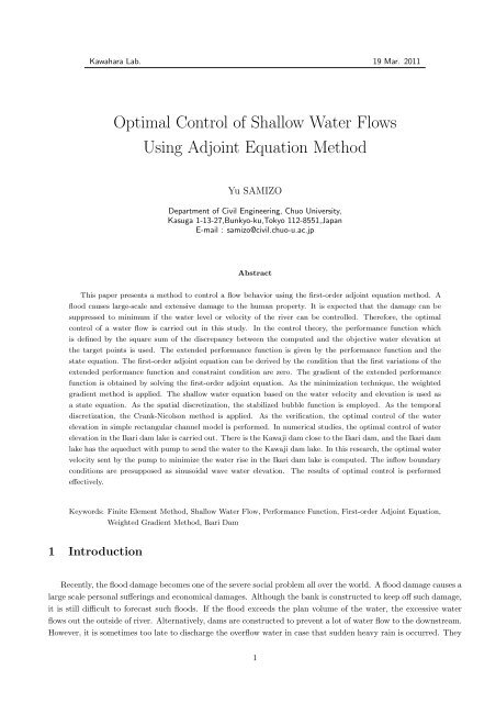
Kawahara Lab. 19 Mar. 2011
Optimal Control of Shallow Water Flows
Using Adjoint Equation Method
Yu SAMIZO
Department of Civil Engineering, Chuo University,
Kasuga 1-13-27,Bunkyo-ku,Tokyo 112-8551,Japan
E-mail : samizo@civil.chuo-u.ac.jp
Abstract
This paper presents a method to control a flow behavior using the first-order adjoint equation method. A
flood causes large-scale and extensive damage to the human property. It is expected that the damage can be
suppressed to minimum if the water level or velocity of the river can be controlled. Therefore, the optimal
control of a water flow is carried out in this study. In the control theory, the performance function which
is defined by the square sum of the discrepancy between the computed and the objective water elevation at
the target points is used. The extended performance function is given by the performance function and the
state equation. The first-order adjoint equation can be derived by the condition that the first variations of the
extended performance function and constraint condition are zero. The gradient of the extended performance
function is obtained by solving the first-order adjoint equation. As the minimization technique, the weighted
gradient method is applied. The shallow water equation based on the water velocity and elevation is used as
a state equation. As the spatial discretization, the stabilized bubble function is employed. As the temporal
discretization, the Crank-Nicolson method is applied. As the verification, the optimal control of the water
elevation in simple rectangular channel model is performed. In numerical studies, the optimal control of water
elevation in the Ikari dam lake is carried out. There is the Kawaji dam close to the Ikari dam, and the Ikari dam
lake has the aqueduct with pump to send the water to the Kawaji dam lake. In this research, the optimal water
velocity sent by the pump to minimize the water rise in the Ikari dam lake is computed. The inflow boundary
conditions are presupposed as sinusoidal wave water elevation. The results of optimal control is performed
effectively.
Keywords: Finite Element Method, Shallow Water Flow, Performance Function, First-order Adjoint Equation,
Weighted Gradient Method, Ikari Dam
1 Introduction
Recently, the flood damage becomes one of the severe social problem all over the world. A flood damage causes a
large scale personal sufferings and economical damages. Although the bank is constructed to keep off such damage,
it is still difficult to forecast such floods. If the flood exceeds the plan volume of the water, the excessive water
flows out the outside of river. Alternatively, dams are constructed to prevent a lot of water flow to the downstream.
However, it is sometimes too late to discharge the overflow water in case that sudden heavy rain is occurred. They
1

causes the dam break and the risk of downstream by a large amount of overflow. In order to prevent such damage,
various provisions should be made.
For example, Kinu river system located in Tochigi prefecture in Japan has a number of dams, and has network
between the Kawaji dam lake and the Ikari dam lake. The Kawaji dam has a larger available storage capacity than
the Ikari dam. In case that the flood that exceeds the acceptable quantity of a dam lake occur, the water is sent
to the other dam lake running through the water tunnel. Herewith, it is possible to prevent the dam break and to
reduce quantity of discharge to the downstream. The optimal control of the intake water has not been carried out
yet. It is necessary to control the intake water velocity to keep the downstream safe.
Consequently, in this research, the verification to control the water elevation at target point in the river is carried
out. Specifying velocity at the boundary in the computational domain, the optimal control of the water elevation
to be as small as possible is carried out by flowing water velocity from the control boundary. The control variable
should be computed so as to minimize the performance function under the constraint of the state equation and
boundary condition. The performance function is defined by the square sum of difference between the computed
and the object value of the water elevations at the target points. The minimization of the performance function
means that computed value becomes as close as possible to the object value. The performance function is extended
by adding inner products between Lagrange multipliers and the state equations. The Lagrange multiplier method
is suitable for the minimization problem with constraint condition. The first-order adjoint equation can be derived
by the state equation and the boundary conditions. As the minimization technique, the weighted gradient method
is applied, which is used widely for the minimization technique. Control variable is updated by the gradient which
is obtained by solving the state and adjoint equations. The shallow water equation are employed as the state
equation. The river and the lake are supposed as a computational domain. As the discretization technique, the
finite element method using the stabilized bubble function in the space direction and the Crank-Nicolson method
in time are applied.
2 State Equation
The non linear shallow water equations are employed as a state equation, which are expressed as follows using
indicial notation and summation convention:
˙u i + u j u i,j + g(η + ξ + H) ,i − ν(u i,j + u j,i ) ,j + fu i = 0, (1)
˙η + {(η + H)u i } ,i = 0, (2)
where u i ,g,η,ξ and H are water velocity, gravitational acceleration, water elevation, bed elevation and water
depth, respectively, ν and f are the coefficient of kinematic eddy viscosity and the bottom friction, respectively.
The boundary conditions shown in Figure 2 are given as follows:
u i = û i on Γ D , (3)
η = ˆη on Γ D , (4)
q = u i n i = ˆq on Γ N , (5)
u i = U i on Γ C , (6)
where the boundaries Γ D ,Γ N , and Γ C are the Dirichlet, Neumann, and control boundaries, respectively and U i is
control variable.
The initial conditions are given as follows:
u i (t 0 ) = û i in Ω, (7)
η(t 0 ) = ˆη in Ω. (8)
2

z
η
u
H
g
ξ
y
x
Figure 1: X-Y-Z Coordinate system
Figure 2: Boundary condition
3

3 Discretization Technique
3.1 Spatial Discretization
For discretization, the finite element method similar to Matsumoto et al.[2003] is used. As for the spatial
discretization of the state equations, the finite element method based on the bubble function interpolation which
is shown in Figure 3 is applied.
u i = Φ 1 u i1 + Φ 2 u i2 + Φ 3 u i3 + Φ 4 ũ i4 , (9)
ũ i4 = u i4 − 1 3 (u i1 + u i2 + u i3 ), (10)
η = Φ 1 η 1 + Φ 2 η 2 + Φ 3 η 3 + Φ 4˜η 4 , (11)
˜η 4 = η 4 − 1 3 (η 1 + η 2 + η 3 ), (12)
Φ 1 = L 1 , Φ 2 = L 2 , Φ 3 = L 3 , Φ 4 = 27L 1 L 2 L 3 . (13)
1
4
2 3
Figure 3: Bubble Function Element
From these discretization technique, the finite element equations of the state equations are expressed as follows:
where
M αβ ˙u βi + A αβγj u βj u γi + S αβi (η β + ξ β + H β ) + D αiβj u βj + fM αβ u βi = 0, (14)
M αβ η˙
β + A αβγi u βi η γ + A αβγi (η β + H β )u βi = 0 (15)
∫
M αβ = (Φ α Φ β )dΩ, (16)
Ω
∫
S αβi = g (Φ α Φ β,i )dΩ, (17)
∫
Ω
A αβγj = (Φ α Φ β Φ γ,j )dΩ, (18)
Ω
∫
∫
D αiβj = ν (Φ α,k Φ β,k )δ ij dΩ + ν (Φ α,j Φ β,i )dΩ. (19)
Ω
Ω
4

3.2 Temporal Discretization
As for the temporal discretization of the state equations, the Crank-Nicolson method is applied:
u n+1
βi
− u n βi
M αβ
∆t
+ A αβγj u n βju n+ 1 2
γi + S αβi
(
η
n+ 1 2
β
+ ξ β + H β
)
+ Dαiβj u n+ 1 2
βi
+ fM αβ u n+ 1 2
βi
= 0, (20)
where
η n+1
βi
− ηβi
n M αβ
∆t
+ A αβγi u n βiη n+ 1 2
γ + A αβγi u n+ 1 2
γi (η β − n + H β ) = 0 (21)
u n+ 1 2
i
= 1 2 (un+1 i + u n i ), (22)
η n+ 1 2 =
1
2 (ηn+1 + η n ). (23)
4 Optimal Control
4.1 Performance Function
In this paper, the control problem is defined to find the control velocity so as to minimize the performance
function under the constraints of the state equation. The performance function J is defined by the square sum
of the discrepancy between the computed and the object value of the water elevations at the target points. The
minimization of the performance function J means that the computed water elevation at the target point becomes
as close as possible to the objective water elevation.
J = 1 2
∫ tf
t 0
∫Ω
(η − η obj )Q(η − η obj )dΩdt, (24)
where Q,η and η obj are weighting diagonal matrix, the computed and the objective water elevation, respectively.
4.2 First-order Adjoint Equation
The Lagrange multiplier method is suitable for the minimization problem with constraint conditions. The
performance function is extended by adding inner products between Lagrange multipliers and the state equations.
The extended performance function J ∗ is expressed as follows:
J ∗ = J +
+
∫ tf
t 0
∫Ω
∫ tf
t 0
∫Ω
u ∗ i { ˙u i + u j u i,j + g(η + ξ + H) ,j − ν(u i,j + u j,i ) ,j + fu i }dΩdt
η ∗ { ˙η + {(η + H)u i } ,i }dΩdt, (25)
where u ∗ i and η∗ denote the Lagrange multiplier for velocity and water elevation, respectively.
The first variation of the extended performance function δJ ∗ is expressed as follows.
δJ ∗ =
+
∫ tf
t 0
∫Ω
∫ tf
t 0
∫Ω
δu i {− ˙u ∗ i − u ∗ i,ju j + u ∗ ju j,i − ν(u ∗ i,jj + u ∗ j,ij) + u ∗ i f − η ∗ ,i(η + H)}dΩdt
δη{− ˙ η ∗ − u ∗ i,ig − η ∗ ,iu i + Q(η − η obj )}dΩdt
5

∫
+ {u ∗ i (t f )δu i (t f ) − u ∗ i (t 0 )δu i (t 0 )}dΩ
Ω
∫
+ {η ∗ (t f )δη(t f ) − η ∗ (t 0 )δη(t 0 )}dΩ
−
+
Ω
∫ tf
t 0
∫ tf
t 0
∫
gu ∗ i δηn i dΓ D dt −
Γ D
∫
∫ tf
t 0
∫
u i η ∗ δηn i dΓ D dt (26)
Γ D
Γ C
{u ∗ i u j + ν(u ∗ j,i + u ∗ i,j) + η ∗ (η + H)δ ij }n j dΓ C dt (27)
The stationary condition is that the first variation of J ∗ should be zero to minimize the performance function.
δJ ∗ = 0. (28)
Then, the first-order adjoint equation eq.(29) and (30), the terminal conditions eq.(31) and (32), and the boundary
conditions eq.(33) and (34) can be obtained:
− ˙u ∗ i − u ∗ i,ju j + u ∗ ju j,i − ν(u ∗ i,jj + u ∗ j,ij) + u ∗ i f − η ∗ ,i(η + H) = 0 in Ω, (29)
− ˙ η ∗ − u ∗ i,ig − η ∗ ,iu i + Q(η − η obj ) = 0 in Ω, (30)
u ∗ i (t f ) = 0 in Ω, (31)
η ∗ (t f ) = 0 in Ω, (32)
u ∗ i = 0 on Γ D , (33)
η ∗ = 0 on Γ D , (34)
b = η ∗ ,in i = 0 on Γ N . (35)
The gradient of the extended performance function with respect to the control variable can be obtained, and it is
expressed by the following form.
grad(J ∗ ) i = {u ∗ i u j + ν(u ∗ j,i + u ∗ i,j) + η ∗ (η + H)δ ij }n j on Γ C . (36)
5 Minimization Technique
5.1 Weighted Gradient Method
In this study, the weighted gradient method is applied as the minimization technique. In the weighted gradient
method, a modified performance function K to which a penalty term is added is used and expressed by the following
equation:
K (l) = J ∗(l) + 1 2
∫ tf
t 0
∫
(U (l+1)
i
Γ C
− U (l)
i )W (l)
ij (U(l+1) j − U (l)
j )dΓ C dt, (37)
where l and W (l)
ij are number of iteration and the weighting parameter , respectively. The penalty term will be
zero, in case that the modified performance function is converged to the minimum value. The minimization of the
performance function is equal to minimize the modified performance function. The following stationary condition
is used to obtain the minimum value of the modified performance function
The control velocity is updated by the following equation.
W (l) U (l+1)
i
δK (l) = 0. (38)
= W (l) U (l)
i
− Grad(J ∗ ) (l)
i (39)
6

5.2 Algorithm
The following algorithm is employed for the computation.
Step 1. Chose the initial control velocity U (0)
i .
Step 2. Solve the state variables u (0)
i
and η (0) using eqs.(1)-(2).
Step 3. Compute the initial performance function J (0) .
Step 4. Solve u ∗(l)
i
and η ∗(l) using eqs.(29)-(30).
Step 5. Solve the gradient using eq.(36).
Step 6. Update the control velocity U (l)
i
Step 7. Solve the state variables u (l+1)
i
using eq.(39).
Step 8. Compute the performance function J (l+1) .
Step 9. Solve u ∗(l+1)
i
and η ∗(l+1) using eqs.(29)-(30).
Step 10. Solve the gradient using eq.(36).
Step 11. Update the control velocity U (l+1)
i
and η (l+1) with the control velocity using eqs.(1)-(2).
using eq.(39).
Step 12. Check the convergence; if ||U (l+1)
i − U i (l)|| < ǫ then stop, else go to step 13.
Step 13. Update a weighting parameter W (l)
ij ;
if J (l+1) < J (l) , then set W (l+1)
ij
else W (l+1)
ij
= 2.0W (l)
ij and go to step 7.
= 0.9W (l)
ij and go to step 4,
6 Verification
In order to confirm that the introduced technique is correct, the verification is carried out using a simple
rectangular channel model. The finite element mesh which has 1203 nodes and 1600 elements is shown in Figure
4. Total length and width are 50[m] and 2[m], respectively. The water depth is 10[m] at whole domain. The time
increment ∆t and the total time are set as 0.005[s] and 5[s]. The coefficient of kinematic eddy viscosity ν and
the bottom friction f are set 0.0[m 2 /s] and 0.0, respectively. The inflow boundary, the control boundary and the
target points are set on the left, on the right and on the center of computational domain, respectively. On the
inflow boundary, the sin wave water elevation is given as Figure 5. The object value of the water elevation at the
target points is set to 0.0[m]. The problem is to find the optimal control velocity on the control boundary so as to
close the water elevation at the target points to object value.
Figure 6 shows variation of the performance function. The performance function converges to 0.0. Figure 8
shows the time history of the water elevation at the target point without control and with control. It is seen that
the water elevation at target points is reduced to object value. Figure 7 shows the time history of the control
velocity.
Therefor, the optimal control of the water elevation at the target points in the simple model is carried out.
7

Figure 4: Finite element mesh, 1203 nodes, 1600 elements
0.1
Inflow water elevation
1
Performance function
0.9
0.08
0.8
0.7
Water elevation [m]
0.06
0.04
Performance function
0.6
0.5
0.4
0.3
0.02
0.2
0.1
0
0 0.5 1 1.5 2 2.5 3 3.5 4 4.5 5
Time [s]
0
0 2 4 6 8 10 12 14 16 18
Iteration
Figure 5: Inflow water elevation
Figure 6: Performance function
0.1
0.09
Control veclocity
0.12
without control
with control
0.08
0.1
0.07
0.08
Control X-velocity [m/s]
0.06
0.05
0.04
0.03
Water Elevation [m]
0.06
0.04
0.02
0.02
0.01
0
0
-0.01
0 0.2 0.4 0.6 0.8 1 1.2 1.4 1.6 1.8 2
Time [s]
Figure 7: Control velocity
0 1 2 3 4 5
Time [s]
Figure 8: Water elevation at the target points
7 Numerical Study
In this study, optimal control of water elevation in the Ikari dam lake which is located in Tochigi prefecture in
Japan is carried out. The Ikari dam lake shown in Figure 10 impounds the water that has flowed from the Oga
river in the upstream, and discharge to the Kinu river in the downstream. There is the hot springs resort area
in the downstream as shown in Figure 9. In case that a flood occurs in upstream of the Ikari dam and the much
water is discharged to the downstream, the hot springs resort area suffers damage. Then, there is the Kawaji dam
close to the Ikari dam, and these two dam lakes can exchange water through the aqueduct. The Ikari dam lake
has the pump system at the aqueduct which can send the water that does not use in the Ikari dam lake and the
water exceed the capacity of the dam. If the over water volume will be discharged from the Ikari dam, it has the
possibility of damaging the hot springs resort area. To reduce the risk, it is necessary to determine the volume to
send the water to the Kawaji dam lake using the aqueduct. In this study, the optimal water velocity sent by pump
system of the aqueduct to minimize the water elevation in the Oga river is carried out.
The finite element mesh is shown in Figure 11. The average of element size is about 10[m]. The total number
of nodes and elements is 2876 and 5215, respectively. The water depth is shown in Figure 12. The time increment
8

is set as 0.2[s]. Total duration time step is 6500. Total time is 1300[s]. The inflow boundary, the outflow boundary,
the control boundary and the target point are set as shown in Figure 2. On the inflow boundary, the boundary
conditions are assumed as flash flood as shown in Figure 13. The object value of water elevation is set to 0.0[m].
The initial condition of the velocity and the water elevation are set 0.0[m/s] and 0.0[m]. The coefficient of kinematic
eddy viscosity ν and the bottom friction f are as 0.01 and 0.01, respectively. The control velocity on the control
boundary is computed by the method presented in this study.
Figure 9: The Ikari dam and the Kawaji dam (Google Map)
sectionNumerical Results
Figure 15 shows variation of the performance function. The performance function converges to about 0.2.
Figure 16 shows the water elevation at the target point without control and with control. It is seen that the water
elevation at target point become lower than without control. Figure 17 and 18 show the time history of the control
X-velocity and Y-velocity, respectively. Figure 19 and 20 show the contour of water elevation in computational
domain without control and with control.
By these results, the optimal velocity at the control point to minimize the water elevation at the target point
is performed.
9

8 Conclusion
In this research, the optimal control of the water elevation in the shallow water flow using the first-order adjoint
equation method is presented. The control velocity is derived so as to minimize the performance function using
the optimal control theory presented in this paper. The water elevation can be as close as object value. As the
future works, determination of the optimal time duration will be presented.
References
[1] J.Matsumoto, T.Umetsu and M.Kawahara, “Stabilized Bubble Function Method for Shallow Water Long Wave
Equation” Int. J. Comp. Fluid Dyn., vol.17(4), pp.319-325, (2003)
[2] M. Shichitake and M. Kawahara, “Optimal Control Applied to Water Flow using Second Order Adjoint
Method”, Int. J. Comp. Fluid dyn. vol22. pp.351-365. (2008)
[3] T.Miyaoka and M.Kawahara, “Optimal Control of Drainage Basin Considering Moving Boundary” Kawahara
Laboratory (2007)
[4] T.Sekine and M.Kawahara, “Computational Water Purification Controls Using Second-order Adjoint Equations
with Stability Confirmation” Kawahara laboratory (2009)
[5] M.Kawahara and K.Sasaki “Adaptive and Optimal Control of the Water Gate of a Dam Using a Finite Element
Method”, Int.J. Comp. Fluid Dyn. vol.7, pp253-273 (1996)
10

Figure 10: The Ikari dam lake
Figure 11: Finite Element Mesh
Figure 12: Water depth
11

2
Inflow water elevation
1
without control
0.8
1.5
0.6
Water elevation [m]
1
Water Elevation [m]
0.4
0.2
0.5
0
0
0 200 400 600 800 1000 1200
Time [s]
-0.2
0 200 400 600 800 1000 1200
Time [s]
Figure 13: Inflow water elevation
Figure 14: Water elevation without control
1
Performance function
1
without control
with control
0.8
0.8
0.6
Performance function
0.6
0.4
Water Elevation [m]
0.4
0.2
0.2
0
0
0 5 10 15 20 25
Iteration
-0.2
0 200 400 600 800 1000 1200
Time [s]
Figure 15: Performance function
Figure 16: Water elevation at target point
1
control X-veclocity
0.4
control Y-veclocity
0.5
0.2
0
Control X-velocity [m/s]
-0.5
-1
-1.5
-2
Control Y-velocity [m/s]
0
-0.2
-0.4
-0.6
-2.5
-3
-0.8
-3.5
0 200 400 600 800 1000 1200
Time [s]
-1
0 200 400 600 800 1000 1200
Time [s]
Figure 17: Control X-velocity
Figure 18: Control Y-velocity
12

Figure 19: Water elevation without control
Figure 20: Water elevation with control
13