Parameter Identification of Manning Roughness Coefficient Using ...

Parameter Identification of Manning Roughness Coefficient
Using Analysis of Hydraulic Jump with Sediment Transport
Akira ISHII
E-mail: a-ki@kc.chuo-u.ac.jp
Abstract
This paper presents a parameter identification of Manning roughness coefficient using the analysis of hydraulic
jump with the sediment transport. To calculate the water flow phenomenon, the shallow water
equation is employed. The friction velocity is applied to the determination of the coefficient of kinematic
eddy viscosity. To calculate the sediment transport, the continuity equation for sand based on the bed-load
quantity is used. The Meyer-Peter Müller equation is used as an equation so as to express the bed-load
quantity. The Crank-Nicolson method is applied to the temporal discretization. The quasi-linear approximation
of advection velocityis given by the Adams-Bashforth formula which has second order accuracy.
The improved bubble element method is applied to the spatial discretization. The Sakawa-Shindo method
is employed for the minimization algorithm.
Key Words : Parameter Identification, Improved Bubble Element, Sakawa-Shindo method
1. Introduction
At the coast of sandy beach including near the
mouse of river,there are problems caused by the
littoral drift in Japan. The littoral drift causes the
deformation of coastal topography because of the
coastal erosion and the sedimentaion. Three major
causes are considered. The first is the decrease
of sandy supply quantity from river because of the
soil-erosion control works and the dams. The second
is a difference in transfer littoral drift quantity
at each place by the coastal flow. The third is an
interception of route of littoral drift which is caused
by building an actual structure. It is considered that
the third case is the most effective against the deformation
of sandy beach. Actually,there are many
actual structures at the coast. And the shape of
actual structure has influence on the deformation of
coastal topography. Therefore,the optimal shape of
actual structure so as to minimize the deformation
of coastal topography are considered.
To consider the sediment transport,such as the littoral
drift which causes the deformation of coastal
topography,the continuity equation for sand based
on the bed-load quantity is used. Before dealing
with the optimal shape problem,the application of
parameter identification to the analysis of shallow
water flow with the sediment transport have to been
considered. This is the purpose of this study. Therefore,the
parameter identification of Manning roughness
coefficient using the analysis of hydraulic jump
with the sediment transport is discussed. The hydraulic
jump needs the effect of friction. The effect
of friction has an influence on the depth of water
and the river-bed. In this study,a value of Manning
roughness coefficient is used as the criteria which
18
expresses the effect of friction.
The shallow water equation and the continuity
equation for sand are reviewed in section 2. In order
to express the bed-load quantity,the Meyer-Peter
Müller equation is used. The spatial discretization
is discussed in section 3. In section 4,the parameter
identification is dealt with. To consider the minimization
problem of performance function,the Lagrange
multiplier method is introduced. The minimization
technique is treated in section 5. The temporal
discretization is discussed in section 6. The
application of parameter identification to the analysis
of shallow water flow with the sediment transport
is verified in section 7. The conclusions are discussed
in section 8.
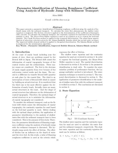
2. State Equation
Y
Z
ξ
η
g
Fig.1 XY-Coordinate System
The shallow water equation and the continuity equation
for sand are used to calculate the water flow
and the sediment transport,respectively. The shallow
water equation and the continuity equation for
sand can be written as follows;
u˙
i + u j u i,j + g ( ξ + η ) ,i
u i
− ν ( u i, j + u j,i ) ,j + fu i = 0, (1)
X

˙ ξ + ξ ,i u i + ξu i,i = 0, (2)
˙η + Λu i,i =0, (3)
where u i , g, ξ and η are the water velocity,the gravitational
acceleration,the water elevation and the
bed elevation,respectively. The coefficient of kinematic
eddy viscosity ν,f and Λ are expressed as
follows;
ν = k l
6 u ∗ ξ, f = u ∗
ξ , Λ= q s
(1 − e ) √ ,
u k u k
where k l , u ∗ , e and q s are the Kalman constant,the
friction velocity,the porosity of sand and the bedload
quantity,respectively. The friction velocity u ∗
is expressed as follows;
√
u ∗ = gn2 uk u k
,
ξ 1/3
where n is the Manning roughness coefficient.
The bed-load quantity q s is determined by a relation
between the tractive force and the limit tractive
force. The tractive force τ 0 is caused by the water
flow. The limit tractive force τ c is expressed as follows;
τ c = σg( ρ s − ρ w ) d m ,
where σ, ρ s , ρ w and d m are the shields parameter,the
density of water,the density of sand and
the sandy average particle size,respectively. The
Meyer-Peter Müller equation is used as an equation
so as to express the bed-load quantity.
If τ 0 >τ c ,
√
1 1
q s =8
ρ w g ( ρ s − ρ w ) ( τ 0 − τ c ) 3 2 .
If τ 0 ≤ τ c , q s =0.
3. Spatial Discretization
3.1 Bubble Function Element
As for the spatial discretization,the interpolation of
bubble function element for the velocity,the water
elevation and the bed elevation fields as shows in
Fig.2 is used. The bubble function element is expressed
as follows;
u i = Φ 1 u i1 + Φ 2 u i2 + Φ 3 u i3 + Φ 4 ũ i4 ,
ũ i4 = u i4 − 1 3 ( u i1 + u i2 + u i3 ),
ξ = Φ 1 ξ 1 + Φ 2 ξ 2 + Φ 3 ξ 3 + Φ 4 ˜ξ4 ,
˜ξ 4 = ξ 4 − 1 3 ( ξ 1 + ξ 2 + ξ 3 ),
where φ e is the bubble function of C 0 continuous
and Φ α ( α = 1 ∼ 4 ) is the bubble function element.
3
s
1
Fig.2
4
2
Bubble Function
Element
r
1.0
s
ω 2
ω 1
ω 3
r
0.0
1.0
Fig.3 Subdivision of
Element
The bubble function is defined by using the
isoparametric coordinates ( r, s ) as shows in Fig.3.
Three triangles ( ω 1 ∼ ω 3 ) is divided at the barycenter
point. The bubble function ofC 0 continuous can
be considered on each sub-triangle as the following
equation;
⎧
⎨ 3(1− r − s ) in ω 1
φ e = 3 r in ω
⎩
2
3 s in ω 3 .
3.2 Improved Bubble Element
The bubble function is capable of eliminating the
barycenter point by using the static condensation.
The discretized form derived from the bubble
function element is equivalent to those from the
SUPG[2]. Therefore,the stabilized parameter which
is derived from the bubble function element is expressed
as follows;
〈 momentum equation for shallow water flow 〉
τ eBui =
〈φ e , 1〉 2 Ω e
A −1
e
1
∆t ‖ φ e ‖ 2 Ω e
+ 1 2 [(ν +˜ν)2 ‖ φ e,j ‖ 2 Ω e
−f ‖ φ e ‖ 2 Ω e
] ,
〈 continuity equations
for shallow water flow and sand 〉
〈φ e , 1〉 2 Ω
τ eBη =
e
A −1
e
1
∆t ‖ φ e ‖ 2 Ω e
+ 1 2 [˜ν ‖ φ e,j ‖ 2 Ω e
] ,
where ˜ν is the stabilized control parameter. From
the criteria for the stabilized parameter in the
SUPG,an optimal parameter can be given as follows;
〈 momentum equation for shallow water flow 〉
η = Φ 1 η 1 + Φ 2 η 2 + Φ 3 η 3 + Φ 4 ˜η 4 ,
˜η 4 = η 4 − 1 3 ( η 1 + η 2 + η 3 ),
Φ 1 = 1 − r − s, Φ 2 = r, Φ 3 = s, Φ 4 = φ e ,
19
τ eBui =
( 1
2 τ −1
es + α ∆t
) −1
,
[ ( ) 2
τes −1 2 | U i |
=
+
h e
( 4ν
h 2 e
) 2 ] 1
2
,

〈 continuity equations
for shallow water flow and sand 〉
where
τ eBη =
( 1
2 τ −1
es
+ α ∆t
) −1
, τ −1
es = 2 | U i |
h e
,
equations. The extended performance function is
expressed as follows;
J ∗ =
∫ tf {
H − λ T ui M ˙u i
t 0
− λ T ξ M ξ ˙
}
− λ T η M ˙η dt, (8)
α = A e ‖ φ e ‖ 2 Ω e
〈φ e , 1〉 2 Ω e
, h e = √ 2A e ,
| U i |= √ u 2 + v 2 + gξ + gΛ,
∫
and Ω e is the element domain, 〈 u, v 〉 Ωe = uvdΩ ,
∫
Ω e
‖ u i ‖ 2 Ω e
= 〈 u, u 〉 Ωe , A e = dΩ . The integral of
Ω e
bubble function is expressed as follows;
〈 φ e , 1〉 Ωe = A e
3 , ‖ φ e,j ‖ 2 Ω e
=3A e g, ‖ φ e ‖ 2 Ω e
= A e
6 ,
g = | Φ α,x | 2 + | Φ α,y | 2 , α =1∼ 3.
4. Parameter Identification
4.1 Performance Function
The parameter identification is defined as finding
the optimal value so as to minimize the performance
function. The performance function is expressed as
follows;
J = 1 2
∫ tf
t 0
{
( ξ − ξ obj ) T Q( ξ − ξ obj )
+(η − η obj ) T R ( η − η obj )
}
dt, (4)
where Q and R are the weighting diagonal matrix.
ξ and η are the water and the bed elevation,respectively.
ξ obj and η obj are the objective water and the
objective bed elevation,respectively.
4.2 Adjoint Equation
The finite element equations of state equations
(1),(2) and (3) can be expressed as follows;
M ˙u + ū j S j u i + gS i ( ξ + η )
+ νH jj u i + νH ji u j
+ fMu i = 0, (5)
M ˙ ξ + ū i S i ξ + ¯ξS i u i = 0, (6)
M ˙η + ΛS i u i = 0. (7)
The Lagrange multiplier method is suitable for
the minimization problem of performance function.
Therefore,the performance function is extended
by the Lagrange multipliers and the finite element
20
where λ ui , λ ξ and λ η express the Lagrange multiplier
for the water velocity,the water elevation and
the bed elevation,respectively. And Hamiltonian H
is defined as follows;
H = 1 2 ( ξ − ξ obj ) T Q ( ξ − ξ obj )
{
T
+λ ui − ū j S j u i − gS i ( ξ + η )
}
− νH jj u i − νH ji u j − fMu i
{
T
+ λ ξ − ū i S i ξ − ¯ξS
}
i u i
{
T
+ λ η − Λ S i u i
}.
To calculate a minimum value of extended performance
function,the first variation of extended performance
function is evaluated. The adjoint equations
and the terminal conditions can be obtained
by δJ ∗ = 0. The adjoint equations and the terminal
conditions are expressed as follows;
Mλ ui = − ∂H
∂u i
,
M λ ξ = − ∂H
∂ξ ,
Mλ η = − ∂H
∂η ,
λ ui = λ ξ = λ η =0 at t = t f .
5.Minimization Technique
5.1 Sakawa-Shindomethod
The Sakawa-Shindo method is applied to the minimization
technique. In this method,the modified
performance function is introduced as adding a
penalty term to the extended performance function.
The modified performance function is expressed as
follows;
K (l) = J ∗(l) + 1 2 ( n(l+1) − n (l) ) T c (l) ( n (l+1) − n (l) ),
where l, n and c (l) are the iteration number for minimization,the
Manning roughness coefficient and the
weighting diagonal matrix,respectively. Applying
to the stationary condition δK (l) = 0,the following
equation can be obtained.
n (l+1) = n (l) + c −(l) ∫ tf
t 0
( ∂H
) (l)
dt, (9)
∂n

where
∂H
∂n =
∂ {
− λ T u
∂n
i
νH jj u i
− λ T u i
νH ji u j − λ T u i
fMu i
}.
The Manning roughness coefficient is renewed by
the equation (9). The initial weighting diagonal matrix
c (0) so that J (1) may be smaller than J (0) is
determined.
5.2 Algorithm
The algorithm of Sakawa-Shindo method is shown
as follows;
1. Set l = 0 and assume the initial Manning roughness
coefficient n (0) .
2. Solve u (l)
i
, ξ (l) , η (l) by using the state equations.
3. Compute the performance function J (l) .
4. Solve the Lagrange multiplier u ∗(l)
i
, ξ ∗(l) , η ∗(l) by
using the adjoint equations.
5. Compute the Manning roughness coefficient
n (l+1)
6. Compute the error norm ɛ = ‖ n (l+1) − n (l) ‖,
and if ɛ

Tab.1 Parameter Value
∆t ( time increment ) 0.02 ( sec )
N ( number of time step ) 3000
k l ( Kalman constant ) 0.41
σ ( shields parameter ) 0.047
ρ s ( density of sand ) 2653 ( kg/m 3 )
ρ w ( density of water ) 1020 ( kg/m 3 )
e ( prosity of sand ) 0.3
d m ( sandy average particle size ) 0.001 ( m )
Tab.2 Coordinate
x y
a 3.0000 0.1000
b 5.5000 0.1000
c 9.0000 0.1000
At first,an objective parameter value of Manning
roughness coefficient is decided. An objective parameter
value is 0.015(s/m 1 3 ). The computational
results which are calculated at this parameter value
are shown from Fig.6 to Fig.9. Moreover,the objective
water and the objective bed elevation are defined
as the water and the bed elevation which are
calculated at this parameter value. To get this objective
parameter value,three objective points ( a,b,
c ) are used as shows in Fig.4. Tab.2 shows x and y
coordinate of three objective points. Next,an initial
parameter value of Manning roughness coefficient
is assumed. In this study,two cases are treated.
As case1,an initial Manning roughness coefficient is
0.030(s/m 1 3). Similarly as case2,an initial Manning
roughness coefficient is 0.013(s/m 1 3 ). According to
the algorithm of Sakawa-Shindo method,the parameter
value is calculated.
Fig.10 and Fig.12 show the variation of performance
function of case1 and case2,respectively.
Fig.11 and Fig.13 show the variation of Manning
roughness coefficient of case1 and case2,respectively.
When the performance function is almost
decreased and converged both cases,the objective
parameter value can be obtained.
8.Conclusions
The purpose of this study is to verify the application
of parameter identification to the analysis of shallow
water flow with the sediment transport. Therefore,
the parameter identification of Manning roughness
coefficient is discussed in this paper. To calculate
the water flow and the sediment transport,the shallow
water equation and the continuity equation for
sand are employed,respectively. The Meyer-Peter
Müller equation is used as an equation so as to express
the bed-load quantity. The Crank-Nicolson
method is applied to the temporal discretization.
The Lagrange multiplier method is applied to the
minimization problem of performance function. The
22
improved bubble element method is applied to the
spatial discretization. The Sakawa-Shindo method
is applied to the minimization technique. When the
performance function is converged,the ob jective parameter
value can be obtained. Thus,the purpose
of this study is achieved. However,as for the parameter
identification of Manning roughness coefficient,
the Manning roughness coefficient can’t be identified
when an initial Manning roughness coefficient
is less than 0.013(s/m 1 3 ). In this study,the shockcapturing
term is applied. When the Lagrange multipliers
are calculated,the parameter of this term is
not well-behaved. Therefore,this parameter is used
as constant. As for the future works,it is necessary
to consider how to treat the shock-capturing term
and the development into the optimal shape problem.
Reference
[1] J. Matsumoto and M. Kawahara,Stable Shape
Identification for Fluid-Structure Interaction
Problem Using MINI Element,Journal of Applied
Mechanics,vol.3, 263-274 (2000).
[2] J. Matsumoto,T. Umetsu and M. Kawahara,
Incompressible Viscous Flow Analysis and Adaptive
Finite Element Method Using Linear Bubble
Function,Journal of Applied Mechanics,vol.2,
223-232 (1999).
[3] Y. Shimizu,M. Fujita and M. Hirano,Calculation
of Flow and Bed Deformation in Compound
Channel with a Series of Verical Drop Spilways,
J. of Hydroscience and Hydraulic Eng.,43,79-84
(1999).
[4] J. Matsumoto,T. Umetsu and M. Kawahara,
Shallow Water and Sediment Transport Analysis
by Implicit FEM,Journal of Applied Mechanics,
vol.1,263-272, (1998).

(m)
2.16
2.14
2.12
2.1
2.08
2.06
2.04
2.02
2
initial bed line
bed line
water elevation
1.98
(m)
0 1 2 3 4 5 6 7 8 9 10
(m)
2.16
2.14
2.12
2.1
2.08
2.06
2.04
2.02
2
Fig.6
t = 6.0(sec)
initial bed line
bed line
water elevation
1.98
(m)
0 1 2 3 4 5 6 7 8 9 10
Fig.8
t = 20.0(sec)
(m)
2.16
2.14
2.12
2.1
2.08
2.06
2.04
2.02
2
initial bed line
bed line
water elevation
1.98
(m)
0 1 2 3 4 5 6 7 8 9 10
(m)
2.16
2.14
2.12
2.1
2.08
2.06
2.04
2.02
2
Fig.7
t = 40.0(sec)
initial bed line
bed line
water elevation
1.98
(m)
0 1 2 3 4 5 6 7 8 9 10
Fig.9
t = 60.0(sec)
Performance Function
Performance Function
9
Performance Function
8
7
6
5
4
3
2
1
0
0 5 10 15 20 25 30 35 40 45
Iteration Count
Fig.10
Performance Function
1.4
Performance Function
1.2
1
0.8
0.6
0.4
0.2
0
0 2 4 6 8 10 12
Iteration Count
Fig.12
Performance Function
Case1
Case2
Manning roughness coefficient
Manning roughness coefficient
0.0325
Manning roughness coefficient
0.030
0.0275
0.025
0.0225
0.020
0.0175
0.015
0.0125
0 5 10 15 20 25 30 35 40 45
Iteration Count
Fig.11
0.015
0.0148
0.0146
0.0144
0.0142
0.014
0.0138
0.0136
0.0134
Manning Roughness Coefficient
0.0132
Manning roughness coefficient
0.013
0 2 4 6 8 10 12
Iteration Count
Fig.13
Manning Roughness Coefficient
23