Computational Accelerator Physics 2002 - Beam Theory Group ...
Computational Accelerator Physics 2002 - Beam Theory Group ...
Computational Accelerator Physics 2002 - Beam Theory Group ...

Create successful ePaper yourself
Turn your PDF publications into a flip-book with our unique Google optimized e-Paper software.
<strong>Computational</strong> <strong>Accelerator</strong> <strong>Physics</strong> <strong>2002</strong><br />
Proceedings of the Seventh International Conference on<br />
<strong>Computational</strong> <strong>Accelerator</strong> <strong>Physics</strong><br />
Michigan, USA, 15–18 October <strong>2002</strong><br />
Edited by<br />
Martin Berz and Kyoko Makino<br />
Institute of <strong>Physics</strong> Conference Series Number 175<br />
Institute of <strong>Physics</strong> Publishing<br />
Bristol and Philadelphia
Preface<br />
This volume contains selected papers from the Seventh International <strong>Computational</strong><br />
<strong>Accelerator</strong> <strong>Physics</strong> Conference that took place 15–18 October, <strong>2002</strong> at Michigan State<br />
University. Following a now well established tradition, the meeting succeeded the conference<br />
in Darmstadt in 2000, and in turn will be followed by the conference in St. Petersburg, Russia<br />
in 2004.<br />
For the refereeing of the papers, we would like to acknowledge the help from a group of<br />
sectional editors that assumed responsibility for certain groups of papers based on their<br />
expertise. Their help was essential for the thorough refereeing and reviewing of the papers.<br />
We would like to thank Bela Erdelyi, Alfredo Luccio, Stephan Russenschuck, Ursula van<br />
Rienen, and Thomas Weiland for assuming responsibility of this important task.<br />
The meeting would not have been possible without help from various sources. We are<br />
grateful for financial support from the US Department of Energy, as well as from Tech-X and<br />
Accel, who as representatives from the commercial world helped defray travel expenses of<br />
graduate students who otherwise may not have been able to attend the meeting. Substantial<br />
support was also provided by the MSU College of Natural Science and the Department of<br />
<strong>Physics</strong> and Astronomy; specifically, we thank Lorie Neuman and Brenda Wenzlick for their<br />
enthusiasm, professionalism, and seemingly never-ending patience.<br />
Kyoko Makino and Martin Berz
Other titles in the series<br />
The Institute of <strong>Physics</strong> Conference Series regularly features papers presented at<br />
important conferences and symposia highlighting new developments in physics and<br />
related fields. Previous publications include:<br />
182 Light Sources 2004<br />
Papers presented at the 10th International Symposium on the Science and Technology<br />
of Light Sources, Toulouse, France<br />
Edited by G Zissis<br />
180 Microscopy of Semiconducting Materials 2003<br />
Papers presented at the Institute of <strong>Physics</strong> Conference, Cambridge, UK<br />
Edited by A G Cullis and P A Midgley<br />
179 Electron Microscopy and Analysis 2003<br />
Papers presented at the Institute of <strong>Physics</strong> Electron Microscopy and Analysis <strong>Group</strong><br />
Conference, Oxford, UK<br />
Edited by S McVitie and D McComb<br />
178 Electrostatics 2003<br />
Papers presented at the Electrostatics Conference of the Institute of <strong>Physics</strong>,<br />
Edinburgh, UK<br />
Edited by H Morgan<br />
177 Optical and Laser Diagnostics <strong>2002</strong><br />
Papers presented at the First International Conference, London, UK<br />
Edited by C Arcoumanis and K T V Grattan<br />
174 Compound Semiconductors <strong>2002</strong><br />
Papers presented at the 29th International Symposium on Compound<br />
Semiconductors, Lausanne, Switzerland<br />
Edited by M Ilegems, G Weimann and J Wagner<br />
173 GROUP 24: Physical and Mathematical Aspects of Symmetries<br />
Papers presented at the 24th International Colloquium, Paris, France<br />
Edited by J-P Gazeau, R Kerner, J-P Antoine, S Métens and J-Y Thibon<br />
172 Electron and Photon Impact Ionization and Related Topics <strong>2002</strong><br />
Papers presented at the International Conference, Metz, France<br />
Edited by L U Ancarani<br />
171 <strong>Physics</strong> of Semiconductors <strong>2002</strong><br />
Papers presented at the 26th International Conference, Edinburgh, UK<br />
Edited by A R Long and J H Davies
Contents<br />
Preface<br />
v<br />
Persistent currents in superconducting filaments due to arbitrary field changes in the<br />
transverse plane<br />
M Aleksa, B Auchmann, S Russenschuck and C Völlinger 1<br />
A simple parallelization of a FMM-based serial beam-beam interaction code<br />
P M Alsing, V Boocha, M Vogt, J Ellison and T Sen 13<br />
Accuracy analysis of a 2D Poisson-Vlasov PIC solver and estimates of the collisional<br />
effects in space charge dynamics<br />
A Bazzani, G Turchetti, C Benedetti, A Franchi and S Rambaldi 25<br />
The COSY language independent architecture: porting COSY source files<br />
L M Chapin, J Hoefkens and M Berz 37<br />
Simulation issues for RF photoinjectors<br />
E Colby, V Ivanov, Z Li and C Limborg 47<br />
Enhancements to iterative inexact Lanczos for solving computationally large finite<br />
element eigenmode problems<br />
J F DeFord and B L Held 57<br />
New numerical methods for solving the time-dependent Maxwell equations<br />
H De Raedt, J S Kole, K F L Michielsen and M T Figge 63<br />
<strong>Beam</strong> simulation tools for GEANT4 (and neutrino source applications)<br />
V D Elvira, P Lebrun and P Spentzouris 73<br />
Muon cooling rings for the ν factory and the µ + µ - collider<br />
Y Fukui, D B Cline, A A Garren and H G Kirk 83<br />
Status of the Los Alamos <strong>Accelerator</strong> Code <strong>Group</strong><br />
R W Garnett 91<br />
3D space-charge model for GPT simulations of high-brightness electron bunches<br />
S B van der Geer, O J Luiten, M J de Loos, G Pöplau and U van Rienen 101<br />
S-parameter-based computation in complex accelerator structures: Q-values and field<br />
orientation of dipole modes<br />
H-W Glock, K Rothemund, D Hecht and U van Rienen 111
viii<br />
AHF booster tracking with SIMPSONS<br />
D E Johnson and F Neri 121<br />
Parallel simulation algorithms for the three-dimensional strong-strong beam-beam<br />
interaction<br />
A C Kabel 131<br />
A parallel code for lifetime simulations in hadron storage rings in the presence of<br />
parasitic beam-beam interactions<br />
A C Kabel and Y Cai 143<br />
Using macroparticles with internal motion for beam dynamics simulations<br />
M Krassilnikov and T Weiland 151<br />
The software ModeRTL for simulation of radiation processes in electron beam<br />
technologies<br />
V T Lazurik, V M Lazurik, G F Popov, Yu V Rogov 161<br />
<strong>Computational</strong> aspects of the trajectory reconstruction in the MAGNEX large<br />
acceptance spectrometer<br />
A Lazzaro, A Cunsolo, F Cappuzzello, A Foti, C Nociforo, S Orrigo, V Shchepunov,<br />
J S Winfield and M Allia 171<br />
Study of RF coupling to dielectric loaded accelerating structures<br />
W Liu, C Jing and W Gai 181<br />
On the map method for electron optics<br />
Z Liu 185<br />
Aspects of parallel simulation of high intensity beams in hadron rings<br />
A U Luccio and N L D’Imperio 193<br />
High-order beam features and fitting quadrupole-scan data to particle-code models<br />
W P Lysenko, R W Garnett, J D Gilpatrick, J Qiang, L J Rybarcyk, R D Ryne,<br />
J D Schneider, H V Smith, L M Young and M E Schulze 203<br />
Muon beam ring cooler simulations using COSY INFINITY<br />
C O Maidana, M Berz and K Makino 211<br />
Solenoid elements in COSY INFINITY<br />
K Makino and M Berz 219<br />
Experience during the SLS commissioning<br />
M Muñoz, M Böge, J Chrin and A Streun 229<br />
Tracking particles in axisymmetric MICHELLE models<br />
E M Nelson and J J Petillo 235
A<br />
ix<br />
<strong>Beam</strong> dynamics problems of the muon collaboration: ν-factories and µ + -µ - colliders<br />
D Neuffer 241<br />
Simulation of electron cloud multipacting in solenoidal magnetic field<br />
A Novokhatski and J Seeman 249<br />
RF heating in the PEP-II B-factory vertex bellows<br />
A Novokhatski and S Weathersby 259<br />
Optimization of RFQ structures<br />
A D Ovsiannikov 273<br />
A multigrid based 3D space-charge routine in the tracking code GPT<br />
G Pöplau, U van Rienen, M de Loos and B van der Geer 281<br />
On the applicability of the thin dielectric layer model for wakefield calculation<br />
S Ratschow, T Weiland and I Zagorodnov 289<br />
COSY INFINITY’s EXPO symplectic tracking for LHC<br />
M L Shashikant, M Berz and B Erdélyi 299<br />
ORBIT: Parallel implementation of beam dynamics calculations<br />
A Shishlo, V Danilov, J Holmes, S Cousineau, J Galambos, S Henderson 307<br />
Vlasov simulation of beams<br />
E Sonnendrücker and F Filbet 315<br />
Space charge studies and comparison with simulations using the FNAL Booster<br />
P Spentzouris, J Amundson, J Lackey, L Spentzouris and R Tomlin 325<br />
Progress in the study of mesh refinement for particle-in-cell plasma simulations and<br />
its application to heavy ion fusion<br />
J-L Vay, _ Friedman and D P Grote 333<br />
Calculation of transversal wake potential for short bunches<br />
I Zagorodnov and T Weiland 343<br />
Author Index 353
Copyright ©2004 by IOP Publishing Ltd and individual contributors. All rights reserved. No part of<br />
this publication may be reproduced, stored in a retrieval system or transmitted in any form or by any<br />
means, electronic, mechanical, photocopying, recording or otherwise, without the written permission<br />
of the publisher, except as stated below. Single photocopies of single articles may be made for private<br />
study or research. Illustrations and short extracts from the text of individual contributions may be<br />
copied provided that the source is acknowledged, the permission of the authors is obtained and IOP<br />
Publishing Ltd is notified. Multiple copying is permitted in accordance with the terms of licences<br />
issued by the Copyright Licensing Agency under the terms of its agreement with the Committee of<br />
Vice-Chancellors and Principals. Authorization to photocopy items for internal or personal use, or the<br />
internal or personal use of specific clients in the USA, is granted by IOP Publishing Ltd to libraries<br />
and other users registered with the Copyright Clearance Center (CCC) Transactional Reporting<br />
Service, provided that the base fee of $30.00 per copy is paid directly to CCC, 222 Rosewood Drive,<br />
Danvers, MA 01923, USA.<br />
British Library Cataloguing in Publication Data<br />
A catalogue record for this book is available from the British Library.<br />
ISBN 0 7503 0939 3<br />
Library of Congress Cataloging-in-Publication Data are available<br />
Published by Institute of <strong>Physics</strong> Publishing, wholly owned by the Institute of <strong>Physics</strong>, London<br />
Institute of <strong>Physics</strong> Publishing, Dirac House, Temple Back, Bristol BS1 6BE, UK<br />
US Office: Institute of <strong>Physics</strong> Publishing, The Public Ledger Building, Suite 929, 150 South<br />
Independence Mall West, Philadelphia, PA 19106, USA<br />
Printed in the UK by Short Run Press Ltd, Exeter
Inst. Phys. Conf. Ser. No 175<br />
Paper presented at 7th Int. Conf. <strong>Computational</strong> <strong>Accelerator</strong> <strong>Physics</strong>, Michigan, USA, 15–18 October <strong>2002</strong><br />
©2004 IOP Publishing Ltd<br />
1<br />
Persistent Currents in Superconducting Filaments<br />
Due to Arbitrary Field Changes in the Transverse Plane<br />
Martin Aleksa, Bernhard Auchmann,<br />
Stephan Russenschuck, Christine Völlinger<br />
Abstract. Magnetic field changes in the coils of superconducting magnets are shielded<br />
from the filaments’ core by so-called persistent currents which can be modeled by means<br />
of the critical state model. This paper presents an semi-analytical 2-dimensional model of the<br />
filament magnetization due to persistent currents for changes of the magnitude of the magnetic<br />
induction and its direction while taking the field dependence of the critical current density into<br />
account. The model is combined with numerical field computation methods (coupling method<br />
between boundary and finite elements) for the calculation of field errors in superconducting<br />
magnets. The filament magnetization and the field errors in a nested multipole corrector<br />
magnet have been calculated as an example.<br />
1. Introduction<br />
The Large Hadron Collider (LHC) [6], a proton-proton superconducting accelerator, will<br />
consist of about 8400 superconducting magnet units of different types, operating in super-fluid<br />
helium at a temperature of 1.9 K. The applied magnetic field changes induce currents in the<br />
filaments that screen the external field changes (so-called persistent currents). The filaments<br />
are made of type II hard superconducting material with the property that the magnetic<br />
field penetrates into the filaments with a gradient that is proportional to the magnitude<br />
of the persistent currents. Macroscopically, these currents (that persist due to the lack of<br />
¤¦¥<br />
resistivity if flux creep effects are neglected) are the source of a magnetization of the<br />
superconducting strands. One way to calculate this magnetization would be to mesh the coil<br />
with finite elements and solve the resulting non-linear field problem numerically by ¡£¢<br />
making<br />
¤¨¥<br />
use of a measured -curve. This approach has two main drawbacks: The numerical field<br />
computation has to be combined with a hysteresis model for hard superconductors, and the<br />
coil has to be discretized with highest accuracy also accounting for the existing gradient ¡§¢<br />
of<br />
the current density due to the trapezoidal shape of the cables, the conductor alignment on the<br />
winding mandrel, and the insulation layers. Hence, we aimed for computational methods that<br />
avoid the meshing of the coil by combining a semi-analytical magnetization model with the<br />
BEM-FEM coupling method [5].<br />
In the straight section of accelerator magnets the magnetic induction is almost perpendicular to<br />
the filament axis. The effect of a magnetic induction parallel to a superconducting filament is<br />
small (see [11]) and has therefore been neglected here. A model to calculate the magnetization<br />
of the superconducting strands is presented, considering external fields that change their<br />
magnitude and direction. For this purpose, the model introduced in [1] has been extended to<br />
account for filament magnetizations non-parallel to the outside field. As in [1], the model does<br />
not attempt to describe the microscopic flux pinning, but applies the critical state model [2]<br />
which states that any external field change is shielded from the filament’ s core by ¢¤¥<br />
layers<br />
of screening currents at ©<br />
critical density . The model differs from other attempts to<br />
describe a superconducting filament’ s response to arbitrary field changes in the transverse
£<br />
<br />
0<br />
<br />
¥<br />
<br />
<br />
<br />
0<br />
<br />
¥<br />
2<br />
g<br />
plane as, e.g., in [8]. It takes into account the dependence of the critical current density on<br />
the applied external fiel and the resulting field distribution in the filament cross-section. As a<br />
consequence, also low field effects such as the peak-shifting (asymmetry in the magnetization<br />
curve for vanishing external field) are reproduced by the model.<br />
The described model is combined with the coupled boundary element / finite element method<br />
(BEM-FEM) [5] which avoids the representation of the coil in the finite element mesh since<br />
the coil is located in the iron-free BEM domain. The fields arising from current sources in<br />
the coil are calculated by means of the Biot-Savart law, while the surrounding ferromagnetic<br />
iron yoke has to be meshed with finite elements. Hence, the discretization errors due to the<br />
finite-element part in the BEM-FEM formulation are limited to the iron-magnetization arising<br />
from the yoke structure. In order to account for the feed-back of the filament magnetization<br />
¤¨¥<br />
on the magnetic field, an -iteration is performed.<br />
The magnetization model is based on the input ¡£¢<br />
¢¤¥<br />
function of the critical © current<br />
density, which represents the material properties of the superconductor, but is independent<br />
of geometrical parameters such as the filament diameter or shape and the ratio of the<br />
superconductor to total strand volume. The method reproduces the hysteretic behavior for<br />
arbitrary turning points in the magnet’s excitational cycle including minor loops and ¡<br />
rotating<br />
external fields.<br />
2. The 1-dimensional magnetization model<br />
For a better understanding of the magnetization model, let us first consider a field change of<br />
the ¢ form is the nominal field strength in some direction<br />
¤£¦¥ ¤<br />
where and ¤<br />
§©¨<br />
perpendicular to the axis of a circular superconducting filament, which we shall call a 1-<br />
¥ §©¨<br />
dimensional field change. This field change induces a shielding-current layer of a relative<br />
thickness called the relative penetration depth, see Fig. 1. It is measured on the scale of<br />
<br />
the relative penetration parameter that is zero on the outside and one in the center of the<br />
filament. The currents are directed as to create a magnetic induction that opposes the applied<br />
field change on the conductor surface, thus shielding the field change from the filament’ s core.<br />
The thickness of the layer depends on the amplitude of the applied field sweep, on the filament<br />
radius, and on the critical current density in the superconducting material.<br />
The generation of a shielding field can be modeled by the perfectly uniform dipole field<br />
produced by two intersecting circles with opposite current densities shifted by the relative<br />
¢ distance<br />
,<br />
<br />
<br />
¢<br />
£! #" <br />
$&%('*)<br />
(1)<br />
',+<br />
" ¢<br />
¢/- -<br />
where is the shielding field, is the filament radius and are the relative penetration<br />
parameters that limit the shielding current layer, [3]. Such pairs of circles are nested inside<br />
concentric circles. This equation will later be used to find a differential equation for the<br />
differential shielding . In Fig. 1 these nested pairs of circles are represented with<br />
finite thickness, notwithstanding the continuous nature of the mathematical model, which<br />
will be introduced in Sec. 3.1. Figure 1 (left) shows the cross-section of a filament after a<br />
1-dimensional change of the external field from to . The nested circles each shield<br />
a fraction of the outside field from the inside, thus increasing 0 ¢ ¤214365 ¤¨¥<br />
©<br />
in the inner circles, as<br />
represented in Fig. 1 (left bottom diagram). The figure also yields a vector representation<br />
¢ ¤ ¢<br />
¥ ¥.-<br />
© <br />
of the 1-dimensional field change and the corresponding shielding effect. The vector ¢ <br />
indicates the shielding magnetic induction as a function of the penetration from the outside<br />
, to the inner boundary of the shielding layer<br />
0 £<br />
), where ¢ 0 ¥2£ <br />
and ¤ ¢ 0 ¥2£<br />
¤87,94:
¥<br />
¢<br />
<br />
<br />
¡<br />
1#3 5 ¢ 0 ¥ <br />
"$# % !<br />
G<br />
<br />
0<br />
<br />
¤214365 <br />
<br />
¡<br />
¡<br />
7 ¢<br />
¥<br />
¥<br />
<br />
¡<br />
<br />
¡<br />
g<br />
3<br />
= <br />
, G<br />
<br />
O H<br />
* O<br />
G <br />
N H<br />
> <br />
* N<br />
@ <br />
<br />
<br />
* O<br />
* N<br />
O H<br />
* O<br />
N H<br />
* N<br />
JG<br />
<br />
* O<br />
* N<br />
* J<br />
*<br />
<br />
G <br />
G <br />
<br />
G<br />
A <br />
<br />
<br />
<br />
<br />
G<br />
<br />
<br />
G <br />
G <br />
G<br />
<br />
<br />
G<br />
Figure 1. Circular superconducting filament in a magnetic induction of fixed direction,<br />
for different penetration states. The individual graphs contain: (a) A schematic view of the<br />
circular filament with inscribed pairs of circles. Orange colors indicate positive currents in<br />
-direction, blue colors indicate negative currents. The color intensity represents the absolute<br />
value of the currents £¥¤¥¦ ¦¨§©© at critical density ; (b) The component of the magnetic<br />
induction over the relative ¡ penetration parameter ; (c) The component ¦¨§© of § over ; § (d)<br />
The vector representation of the shielding problem in the -plane; and ¡ ¡<br />
¡ denote the <br />
external field vector and the shielding field vector at ¡ penetration , , respectively; § (e)<br />
¦¨§©<br />
The shielding currents £¥¤¥¦ ¦¨§©© at critical density in the cross-section. Left: Penetration to<br />
a relative § penetration depth of . (§ Right: Full penetration ).<br />
¤ ¢ ¥ ¤27,94:; ¢ <br />
<br />
(<br />
¥<br />
<br />
<br />
<br />
<br />
¢¤ ¢<br />
©<br />
¥¥<br />
( <br />
¢ ¤ 0<br />
<br />
¥<br />
<br />
¢<br />
¤ ¤27 <br />
¢ 0<br />
(<br />
(<br />
), where . The absolute value of depends in a non-linear<br />
way on the penetration parameter (see -relation in Eq. (6) and on the applied field<br />
change.<br />
The right hand side of Fig. 1 shows the situation where a larger field change is applied to the<br />
filament surface. The entire cross-section contains shielding currents of critical density which<br />
are, however, unable to completely shield the field from the inside. The field has thus fully<br />
penetrated the filament ). In the vector representation, points from the induction<br />
at the filament surface to the value of the induction at the center of the filament<br />
.<br />
Fig. 2 (left) shows the case where the magnetic induction outside the filament is ramped up to<br />
(previously denoted ) and subsequently reduced to . A new layer of shielding<br />
currents is generated, leaving the remaining inner layers untouched. The new field change is<br />
again shielded from the filament’ s core. The shielding vector is now to oppose the<br />
new field change. It further has to fulfill continuity requirements on the outer ) and<br />
inner boundary of the new current layer<br />
):<br />
¤ ¢ 0 ¥ <br />
¤21#3 5 ;<br />
(2)<br />
<br />
¥ <br />
¤21#3 5 ;<br />
1#3 5 ¢ <br />
<br />
¥ <br />
<br />
¤27 ;<br />
<br />
¥&<br />
(3)<br />
¤ ¢
¥<br />
G<br />
¥<br />
G<br />
¥<br />
4<br />
With given 7 ¤27<br />
and , the mathematical problem consists in the determination of a<br />
5<br />
penetration parameter and the corresponding shielding vector that satisfies the Eqs. ¤21#3 (2)<br />
<br />
and (3). For the 1-dimensional field change this task has been discussed 5 1#3 in [1].<br />
O H<br />
O H<br />
* N<br />
N H<br />
<br />
<br />
N H<br />
* N<br />
<br />
<br />
* O<br />
* O<br />
<br />
G <br />
<br />
<br />
G <br />
<br />
G<br />
* O<br />
J @<br />
J A M<br />
* @ * A M<br />
* N<br />
<br />
<br />
<br />
<br />
G<br />
* @<br />
J @<br />
* O<br />
* N<br />
* A M J A M<br />
<br />
G <br />
<br />
G <br />
<br />
G<br />
<br />
<br />
G<br />
Figure 2. Sequel to Fig. 1 (right). Different 1-dimensional field changes applied to a fully<br />
penetrated superconducting filament. Left: The diminution of the external field causes the<br />
creation of a new current layer of relative thickness with opposite current densities. Right:<br />
The outer field changes sign, causing the new current layer to completely erase the previous<br />
layer ( ). The gray part of the ¡£¢ ¤<br />
vector represents ¡£¢ ¤ , the part of the shielding<br />
magnetic induction that has been replaced by the new shielding layer ¦¥¨§© .<br />
Figure 2 (right) shows a case where a field changes wipes out the previous current layer(s)<br />
entirely. This happens, if the field change is too large (or the field is turned into a direction<br />
that does not allow for an intersection of shielding vectors, see Sec. 3). It further shows that<br />
¢ ¥ ¤ ¥ 0<br />
<br />
<br />
the critical current density reaches its maximum at where the shielding<br />
effect is biggest and the ¤<br />
curve has the steepest inclination.<br />
¢ ¤<br />
¢ <br />
3. Persistent Currents Model for 2-dimensional field changes<br />
The more general case of a magnetic induction that changes its absolute value and direction<br />
is discussed now. We shall denote the underlying model therefore as “2-dimensional” or the<br />
“vector magnetization model”. Starting again from the situation described in Fig. 1 (right), a<br />
clockwise rotation and diminution of the magnetic induction is now studied. It can be expected<br />
from the results presented in Section 2 that a new shielding-current layer of relative thickness<br />
is created to oppose the change of the induction. Of course, the continuity equations (2)<br />
<br />
and (3) also have to hold for rotational field changes.<br />
Figure 3 (left) illustrates the case. The shielding vector 14365 ¢ points to ¤27 ; 7 ¢<br />
.Itis<br />
directed as to shield field changes from the filament’ s core in accordance with the continuity
G<br />
1#3 5 ¢ <br />
<br />
<br />
¥<br />
<br />
<br />
<br />
¥<br />
<br />
<br />
<br />
G<br />
5<br />
* N<br />
O H<br />
O H<br />
N H<br />
G G <br />
* N<br />
N H<br />
<br />
<br />
* O<br />
* O<br />
J @<br />
J A M<br />
= A M<br />
= A M<br />
> A M<br />
J A M<br />
J @<br />
* A M<br />
* O<br />
* N<br />
* @<br />
= @<br />
* @<br />
* A M<br />
<br />
G <br />
<br />
G <br />
<br />
G<br />
* O<br />
* N<br />
> A M<br />
<br />
<br />
<br />
G<br />
> @<br />
Figure 3. Left: Sequel to Fig. 1 (right). The<br />
¡ ¥¨§©<br />
outer field is decreased and<br />
¥¨§©¢¡<br />
turned by<br />
¤ with respect to the previous excitation step<br />
¡<br />
¡ ¢ ¤ . A new current layer is created<br />
¡ ¢<br />
with § relative thickness , that shields the field change from the filament’s<br />
¡ ¥¨§©<br />
core. Right:<br />
is increased and rotated with<br />
¡<br />
¡ ¢ ¤ respect to . The field change fully penetrates the crosssection.<br />
In the vector representation, the shielding vector points to the arrowhead of the<br />
¦¥¨§©<br />
old<br />
<br />
¡ ¢ ¤ shielding vector .<br />
equations (2) and (3). The magnetic induction in the filament cross-section is, thus, given by<br />
¥ ¤£<br />
¤214365(;<br />
¥ 0¦¥<br />
¥ & (4)<br />
<br />
<br />
( <br />
<br />
Similar to the case presented in Fig. 2 (right), the current layer resulting from the outer<br />
field change shown in Fig. 3 (right) penetrates the entire cross-section. Again, the previous<br />
shielding-current layer is completely removed ). As the effects are computed for<br />
successive excitational conditions and the computational results ought to be independent of<br />
the step sizes of these excitations, the vector for points to the arrowhead of .<br />
This behavior is illustrated in Fig. 4.<br />
¤ ¢<br />
¤27 ;<br />
7 ¢<br />
¥ <br />
3.1. Mathematical description of the vector magnetization model<br />
Most magnetization models for superconducting filaments (e.g. [11]) neglect the fielddependence<br />
of the critical current density © . This is reasonable only if the excitational field is<br />
large compared to the field generated by the filament magnetization (i.e., all the filaments are<br />
fully penetrated). There are, however, regions in superconducting coils that yield a magnetic<br />
induction in the transverse plane that is close to zero even at nominal level. Strands that are<br />
positioned in these regions - the vorteces of the magnetic induction - are not fully penetrated<br />
during the entire ramp cycle of a magnet. The model introduced in this paper includes varying<br />
current densities inside the filament and calculates the continuous course of the magnetic field<br />
over the filament cross-section by means of a differential approach. The model is, therefore,<br />
suited to describe also low-field effects such as the peak-shifting, see Fig. 4. The following<br />
approach was adopted to derive the mathematical model:<br />
§ A differential equation for the course of the magnetic field is derived, based on the<br />
equation for the perfectly uniform dipole field produced by a pair of intersection circles,<br />
compare Eq. (1).
§<br />
§<br />
§<br />
§<br />
§<br />
§<br />
<br />
<br />
<br />
¥ <br />
<br />
¥ <br />
¥<br />
¥<br />
<br />
<br />
¤<br />
<br />
¥<br />
<br />
<br />
<br />
<br />
<br />
<br />
¥<br />
&<br />
<br />
<br />
<br />
6<br />
* O<br />
* O<br />
* O<br />
* @<br />
* A M<br />
J A M<br />
J @<br />
J @<br />
J A M<br />
J @<br />
J A M<br />
* @<br />
* A M * @<br />
* A M<br />
= <br />
> <br />
Figure 4. Vector representation of steps of different sizes, following an increase and rotation<br />
of the magnetic induction on a filament’s surface (dashed line). This plot is to illustrate why,<br />
after a large step, (c), the shielding<br />
¥ §©<br />
vector has to point to the arrowhead<br />
<br />
¡ ¢ ¤ of : Increasing<br />
the step size, the moment of full penetration of the field (§ ) is reached in (b). Assume<br />
now that the step size is being infinitesimally increased. In order to avoid any incontinuity of<br />
the results due to a choice of step sizes, the new shielding vector must point to the arrow head<br />
of the old vector. Applying the same reasoning to a larger step, (c), it can be seen that letting<br />
¦¥¨§©<br />
point to the arrow head<br />
<br />
¡ ¢ ¤ of is the appropriate approximation of a series of successive<br />
infinitely small steps along the dashed line.<br />
To obtain a solveable differential equation, the fit function for the critical current density<br />
is approximated around the working point.<br />
A set of differential equations for the - and ¡ a -components is derived, to describe<br />
arbitrary field changes in the transverse plane.<br />
The shielding induction vector ¢ is introduced to describe the course of the induction<br />
over the cross-section.<br />
One differential equation for ¢ <br />
¥ ¢ ¥ <br />
is obtained. Solving the equation yields the<br />
inverse relation ¢ ¥<br />
. <br />
With this solution at hand, the penetration parameter of a new shielding current layer can<br />
be determined by solving an equation system, given by the continuity requirements in<br />
¢ ¤ ¢ ¥ ¥<br />
Eqs.(2-3).<br />
relation, the<br />
magnetization of the filament can be calculated.<br />
Given the limits of each current layer and the respective © <br />
The critical current density as a function of the magnetic induction ¢ <br />
the following fit function [4], where ¤ ¤ :<br />
<br />
¤ ¢<br />
<br />
¥<br />
¥ <br />
is given by<br />
¤<br />
¢ ¢ ¥¤ <br />
¥ §¦ ¨ ¥<br />
£¢<br />
£¢<br />
(5)<br />
§¦ ¨<br />
3<br />
¢¤ ¢<br />
¥ ¥ ©©<br />
<br />
<br />
<br />
¤ ¢<br />
¤ ¢<br />
The fit parameters for the LHC main-magnet cables are a reference current © ©<br />
0 ¤"!<br />
$# &&%'<br />
density<br />
, a critical temperature of<br />
<br />
(at 4.2 K and 5 T), an upper critical field ¤ £¢<br />
<br />
¢ <br />
<br />
© <br />
¢¤<br />
3<br />
(¢<br />
<br />
. /<br />
$ & $<br />
1<br />
<br />
¢ ¢¤ ¥ ¥32 4 ¥ ¢<br />
¤ that©<br />
687,9<br />
<br />
:¤
Substituting )<br />
.<br />
1#3<br />
¤¦¥ ¢<br />
¢ <br />
<br />
-<br />
<br />
<br />
)<br />
¢<br />
)<br />
<br />
<br />
&<br />
¥<br />
'<br />
<br />
<br />
<br />
¥<br />
<br />
<br />
<br />
¥<br />
©<br />
¥¡ ¢¤27,94:<br />
¤ ;<br />
¤27,94:<br />
¢/<br />
¥<br />
<br />
¥<br />
¤<br />
; ;<br />
<br />
<br />
¤27,94:<br />
<br />
<br />
¢ ¤ 7,94: .<br />
/ ¢.<br />
<br />
<br />
¥!;<br />
<br />
<br />
¢¤27,94: ¥ ¤<br />
¤ ;<br />
¢ ¤27,9 :,.<br />
¥<br />
$6&<br />
; ¤ ;<br />
; ;<br />
¤27,94:<br />
/<br />
.<br />
<br />
+<br />
<br />
-<br />
$<br />
<br />
<br />
/<br />
¥<br />
<br />
'<br />
&<br />
<br />
<br />
<br />
¥<br />
¥<br />
/<br />
/<br />
<br />
&<br />
¤27,94:<br />
$<br />
7,94: $ ¤27,94: <br />
#<br />
; .<br />
#<br />
$<br />
<br />
32 .54¡4<br />
&<br />
<br />
¢ ¤27,9 :7(.<br />
¥ <br />
<br />
&<br />
7,94:<br />
398<br />
<br />
¥<br />
<br />
7<br />
point ¤27,9 : <br />
with the following function ( <br />
¤27,94:<br />
is constant):<br />
¢ ¤ ¥ 9<br />
(6)<br />
¤27,94:<br />
From Eq. (1) for the perfectly uniform dipole field produced by a pair of intersection circles,<br />
¢ ¤<br />
a system of differential equations for the field change within the filament can now be<br />
-<br />
© <br />
<br />
¢<br />
¥£¢<br />
¢<br />
derived:<br />
- ¤¦¥ ¢<br />
!<br />
¢ ¤27,94: ¥©¨ ¤<br />
¤ ¥<br />
¢.<br />
<br />
/ ;<br />
¥<br />
-<br />
¥<br />
(7)<br />
¢.<br />
- ¤¦§ ¢<br />
¢<br />
<br />
The angles are defined in Fig. 3. The geometry factor ¨ $ "<br />
¥<br />
$ ¥ 0 &.# ¢<br />
, where "<br />
"<br />
denotes the filament radius, accounts for the little spaces that are left when a round filament is<br />
filled with a series of intersecting circles inscribed in concentric circles (instead of intersecting<br />
ellipses that would avoid these spaces but which could not be inscribed in concentric circles,<br />
see Fig. 1 (left) and [1]). By setting<br />
<br />
; ¢<br />
¥<br />
¢.<br />
¥<br />
(8)<br />
¤¦§ ¢<br />
! "# %<br />
¢.<br />
! "$# %<br />
¥<br />
"$# %<br />
!<br />
! #" <br />
and hence<br />
¤ ¢<br />
¥ ;<br />
7,94: $ ¤27,94: ¢<br />
<br />
<br />
¥% ¢.<br />
we can derive from Eq. (7) a differential equation for ¢ <br />
<br />
¢ ;<br />
:<br />
(9)<br />
$ <br />
<br />
<br />
¥<br />
'& - ¤ ;<br />
7,94: $ ¤27,94: ¢<br />
<br />
<br />
¥%(. yields<br />
¥%( ¢.<br />
¥<br />
¢ <br />
¥ <br />
¤ ¢ ¤27,94: ¥©¨ -<br />
(10)<br />
¤ ¢¤27,9 : ¥*¨ -<br />
(11)<br />
<br />
; ¤ 7,94: ¥ ¢.<br />
A solution for and hence for<br />
Mathematica computer program [7]):<br />
¥<br />
is found by integrating Eq. (11) (using the<br />
;<br />
)<br />
!<br />
¢¤87,94: .<br />
¥<br />
¤ ¢ ¤27,94: ¥©¨<br />
<br />
¤27,94:,¢.<br />
¥.- $;<br />
10 <br />
¥<br />
<br />
<br />
$<br />
<br />
<br />
(12)<br />
<br />
.<br />
10 <br />
<br />
10 where denotes the Gauss’ Hypergeometric function. The algorithm for the<br />
¤<br />
10 implementation of in the program language C was based on [9].<br />
A system of equations can now be established for the problem of finding a relative<br />
penetration depth that fulfills the Eqs. (2) and (3) or, equivalently, the problem <br />
of finding<br />
¢ 5 ¥ 14365<br />
<br />
7 ¢ ¥ 1#3 5 7 <br />
and . Obviously it is required that<br />
<br />
<br />
<br />
1#3 5 ¥ ¢¤27 7 5 7 ¥<br />
¢¤81#3 5 1#3<br />
(13)<br />
. .
$ <br />
<br />
<br />
¥<br />
¥<br />
¢¡¤£<br />
<br />
<br />
¢ ¤27,94: ¥<br />
<br />
¢ <br />
&<br />
<br />
<br />
¥<br />
<br />
<br />
¥<br />
5<br />
/1#3<br />
¥<br />
/7<br />
¥<br />
<br />
<br />
/7 ¥<br />
¢ ¤27,94: .<br />
<br />
$ <br />
<br />
$<br />
<br />
-<br />
-<br />
<br />
<br />
¥<br />
¢¡ ¥ <br />
<br />
<br />
¥<br />
<br />
¥<br />
<br />
<br />
8<br />
Moreover, the continuity equation (3) yields<br />
¤21#3 5<br />
/14365<br />
<br />
/14365<br />
; 14365<br />
¢.<br />
14365 <br />
/1#3 5 ¥<br />
¢.<br />
(/7 <br />
; ¤27 <br />
/<br />
/7 <br />
7 <br />
( ¢.<br />
&<br />
(14)<br />
Given the quantities<br />
.7 ¤27 <br />
<br />
, and/7<br />
, the system of equations (13) and (14)<br />
/14365 <br />
can be solved ¤ 1#3 5 1#3 5 1#3 5<br />
for the and by means of a Newton algorithm.<br />
Eventually, to find the distribution of the magnetic induction in the filament cross-section, 7 <br />
<br />
<br />
unknowns.<br />
see<br />
Eq. (9), the inverse relation of Eq.<br />
<br />
<br />
(12), , is required. It is obtained from the<br />
Newton algorithm, using recursions of the form. 7,94: ¤ ¢ <br />
7<br />
7<br />
/ ¢.<br />
14365<br />
¢¡ <br />
¢¤27,94: ¥* <br />
7,94: $ ¤27,9 : ¢¡ ¢.<br />
¥ ; ¡<br />
<br />
(15)<br />
!<br />
¤ <br />
0 & && <br />
denoting the index of the iteration step. An appropriate starting value is<br />
<br />
required.<br />
with¥<br />
From Fig. 3 it is easy to see<br />
;<br />
that field changes on the outside of the filament effect the<br />
¦<br />
of§©¨¦ creation distinct shielding-current layers between the relative penetration parameter<br />
values £<br />
and , ¨¨§ . The indices and<br />
; <br />
correspond to what previously has been<br />
subscripted as ’old’ and ’new’.<br />
<br />
Provided the semi-analytic expression for the magnetic induction ¢ inside the filament,<br />
¢¤ ¢ ¥¥<br />
can be<br />
derived. The vector of the entire filament’ s magnetization ¤ equals the geometric sum of the<br />
¡<br />
the magnetization due to a layer of shielding currents of critical © density<br />
magnetization vectors generated by the individual current layers,<br />
¡<br />
¥.-<br />
(16)<br />
where<br />
¢<br />
denotes the magnetization contribution of a shielding current layer of relative<br />
thickness at .<br />
, subsequently denoted<br />
-<br />
. We obtain for the magnetization of one shielding-current layer<br />
'<br />
The direction of follows the direction of the shielding vector <br />
¢<br />
¡<br />
<br />
<br />
¡<br />
<br />
¡<br />
% ' +<br />
¢<br />
¢ ¤ ¢<br />
¥ ¥ ¢ <br />
¥ <br />
© <br />
<br />
<br />
#"<br />
%' +<br />
¡<br />
<br />
#"<br />
(17)<br />
'<br />
%(' +<br />
where ¤ ¢ <br />
is given in Eq. (9). Generally, Eq. (17) is evaluated numerically. An analytical<br />
approximation exists for outer fields being substantially larger than the shielding induction,<br />
¢ ¤27,94: ¥<br />
<br />
<br />
¢<br />
£ ¥ <br />
which is used whenever possible in order to accelerate the function<br />
<br />
evaluation.<br />
'<br />
; ¤ ¢<br />
4. Simulations of a single filament subjected to field changes<br />
at &)<br />
The result is scaled for a strand with a filling factor $&0)%<br />
takes into account the copper to superconductor ratio of the multi-filament wire. Figure 4<br />
presents computations of 1-dimensional field changes between ¤ 7,94: 0 $ and -2 T. The<br />
<br />
which<br />
&%<br />
The computations in this section are presented for one filament with a radius "<br />
m<br />
+<br />
.
0<br />
9<br />
model reproduces the typical hysteretic behavior of superconducting filaments, as discussed<br />
in [1].<br />
Note that the so-called virgin curve joins the hysteresis slope in the point where the outer<br />
field has fully penetrated the filament cross-section (and which is not the point of maximum<br />
magnetization). At every point the magnetization vector opposes the applied field change.<br />
Consequently the lower branch of the hysteresis loop (up-ramp) is called the shielding branch<br />
and the upper branch (down-ramp) is called the trapping branch. It can also be seen that the<br />
filament magnetization increases as the outer field tends to zero and decreases for larger outer<br />
¡<br />
.<br />
inductions. This effect is due to the -dependence of the critical current density © <br />
¢¤ ¥<br />
¤<br />
The fact that the actual peak of the magnetization is shifted from is discussed in detail<br />
in [1].<br />
A similar case for the vector magnetization model is shown in Fig. 6. The left hand side<br />
0 ¤¤£<br />
diagram shows a clockwise rotating excitation field that goes through the origin in the ¤ ¥ ¤ ¤ § -<br />
plane ( ). As for the first excitation steps, the filament’ s response (shown in the<br />
right diagram of Fig. 6) is very similar to the 1-dimensional field change. The magnetization<br />
opposes exactly the applied field. As the outer field further increases in absolute ¤27,94: £<br />
value, the<br />
magnetization decreases due to the field dependence of the critical current density. At full<br />
penetration the magnetization curve meets the closed 2d-hysteresis<br />
¡ <br />
loop. The maximum of<br />
¤27,9 :<br />
is reached at the completion of each turn in the excitational field, where is zero.<br />
<br />
5. Combining the model with numerical field calculation<br />
For the calculation of field errors in superconducting accelerator magnets with a ferromagnetic<br />
yoke, the magnetization model is combined with the coupling method between boundary<br />
and finite elements BEM-FEM which accounts for the local saturation effects in the yoke,<br />
µ 0 M<br />
0.15<br />
0.1<br />
0.05<br />
trapping<br />
0<br />
-0.05<br />
virgin<br />
shielding<br />
-0.1<br />
-0.15<br />
-2 -1.5 -1 -0.5 0 0.5 1 1.5 2<br />
B<br />
Figure 5. Computed magnetization curve for one filament, scaled by the filling <br />
factor<br />
¦¨§© ¤ ¦ ¤ ). The excitational field is represented on the x-axis, the<br />
(¡ £¢¥¤<br />
corresponding magnetization on the y-axis. Note that the maximum of the magnetization is<br />
not exactly at zero excitation but slightly shifted from it. This effect is called “peak-shifting”<br />
and is confirmed by measurements.
10<br />
By<br />
0.1<br />
µ 0 My<br />
0.06<br />
0<br />
0.04<br />
0.02<br />
-0.1<br />
0<br />
-0.2<br />
-0.02<br />
-0.04<br />
-0.3<br />
-0.06<br />
-0.4<br />
-0.08<br />
-0.1<br />
-0.5<br />
-0.12<br />
-0.5 -0.4 -0.3 -0.2 -0.1 0 0.1<br />
Bx<br />
-0.12 -0.1 -0.08 -0.06 -0.04 -0.02 0 0.02 0.04 0.06<br />
µ 0 Mx<br />
Figure 6. Rotational field excitation of one filament, scaled by the (¡ <br />
filling factor<br />
¦ §© <br />
<br />
¤ ¦ ¤ ). Two complete turns have been computed. Left: The<br />
¢ ¤<br />
external field follows a circular, clockwise path that goes through the origin in the -<br />
<br />
plane. Right: The filament’s response in terms of magnetization; A virgin curve and a closed<br />
<br />
hysteresis slope can be identified.<br />
[5]. The BEM-FEM formulation has the major advantage that the coil does not have to be<br />
meshed in finite elements since it is positioned in the iron-free BEM domain. The coil can<br />
therefore be modeled with the required accuracy taking insulation layers, cable keystoning,<br />
and conductor placements into consideration. The fields arising from the source currents in<br />
the superconducting coil and those resulting from the induced superconductor magnetization<br />
can be calculated analytically by means of the Biot-Savart Law. The field generated by the<br />
magnetization of the superconducting strands at each strand position is added to the computed<br />
sum of the source fields from the superconducting coil and the contributed magnetic induction<br />
which results from the non-linear iron yoke.<br />
In order to calculate global shielding effects in the coil (in particular at low excitational<br />
field) the feed back of the persistent currents on the excitational field is calculated by means<br />
¤¨¥<br />
of an -iteration on the strand level. For that, an algorithm is implemented, that<br />
controls the convergence of the - ¡£¢<br />
and -components of the magnetization vectors seperately,<br />
¡<br />
since convergence in magnitude only does not exclude rotation. The combination of the<br />
magnetization model with numerical field computation follows the method described in [10]<br />
for the 1-dimensional model.<br />
Fig. 7 shows the field plots of the combined octupole decapole spool-piece corrector (MCDO)<br />
for the LHC. A somewhat academic excitational cycle is considered (which will serve the<br />
purpose of validating the model with measurements). First the decapole is ramped up to<br />
0.25 of its nominal field value. Then the octupole is powered up to its nominal field value<br />
(100 A) which creates the asymmetric field in the magnet. Then the octupole field is ramped<br />
repeatedly up and down between +100 and -100 A. The latter stages are displayed in Fig. 7.<br />
This excitation creates a field change in a particular strand which is displayed on the left hand<br />
side of Fig. 8 together with the resulting magnetization on the right.<br />
Fig. 9 shows the 7 and ¤ ¨ field component for the MCDO magnet with the ramp cycle<br />
¤<br />
described as above. The field errors are the Fourier series components (in Tesla) of the radial<br />
field at a reference radius " of 17 mm. The field in the aperture can be calculated from the
0. - 0.024<br />
<br />
<br />
<br />
¢£¢ ¥<br />
"<br />
11<br />
|Btot| (T)<br />
|Btot| (T)<br />
0.435 - 0.459<br />
0.410 - 0.435<br />
0.386 - 0.410<br />
0.362 - 0.386<br />
0.338 - 0.362<br />
0.314 - 0.338<br />
0.290 - 0.314<br />
0.266 - 0.290<br />
0.242 - 0.266<br />
0.217 - 0.242<br />
0.193 - 0.217<br />
0.169 - 0.193<br />
0.145 - 0.169<br />
0.121 - 0.145<br />
0.097 - 0.121<br />
0.073 - 0.097<br />
0.048 - 0.073<br />
0.024 - 0.048<br />
0. - 0.024<br />
Figure 7. Field plots for the different excitations of the combined decapole octupole corrector<br />
magnet. First the decapole (outer layer coil) is ramped up to about 0.25 of its nominal field<br />
value. Then the octupole (inner layer coil) is powered up to its nominal field value (100<br />
A) which results in the assymmetric field in the magnet as displayed on the left hand side.<br />
Subsequently the octupole field is ramped up and down between +100 and -100 A. This is<br />
a somewhat academic excitational cycle but it will serve the purpose of validating the model<br />
with measurements.<br />
relation<br />
§<br />
<br />
<br />
¤ ¢ ; ¤ ¤¦¥<br />
<br />
;<br />
<br />
¡<br />
¢ where<br />
that, for symmetry reasons, the numerical calculation of the MCDO magnet’s field without<br />
the persistent current effects does not have any 7 or ¤ component.<br />
¤<br />
¥<br />
<br />
<br />
(18)<br />
;<br />
( [6]. The ¤ <br />
are called the normal and the ¡ <br />
the skew components. Note<br />
By<br />
0.25<br />
0.2<br />
µ 0 My<br />
0.06<br />
0.04<br />
0.15<br />
0.02<br />
0.1<br />
0.05<br />
0<br />
0<br />
-0.02<br />
-0.05<br />
-0.04<br />
-0.1<br />
-0.06<br />
-0.15<br />
-0.15 -0.1 -0.05 0 0.05 0.1 0.15 0.2 0.25<br />
Bx<br />
-0.06 -0.04 -0.02 0 0.02 0.04 0.06<br />
µ 0 Mx<br />
Figure 8. Left: Excitational field of one filament in the MCDO combined corrector magnet.<br />
Right: The filament’s response in terms of magnetization. The filament in question is situated<br />
at the “two o’clock”position in the outer coil (decapole), compare Fig. 7
0 20 40 60 80 100 120 140<br />
12<br />
x 10 -3 B3.<br />
x 10 -4 B7.<br />
-0.04<br />
0.14<br />
0.12<br />
-0.06<br />
0.1<br />
-0.08<br />
0.08<br />
-0.1<br />
0.06<br />
0.04<br />
-0.12<br />
0.02<br />
-0.14<br />
0<br />
Step 0 20 40 60 80 100 120 140<br />
Step<br />
Figure 9. Field errors (left right in Tesla at a reference radius of 17 mm) as a function<br />
of the excitation step. First the decapole (outer layer coil) is ramped up to about 0.25 of its<br />
¡ ¡£¢<br />
nominal field value (step 10). Then the octupole (inner layer coil) is powered up to its nominal<br />
field value (100 A, step 20). Subsequently the octupole field is ramped up and down between<br />
+100 (step 20, 60, 100) and -100 A (step 40, 80, 120).<br />
6. Conclusions<br />
A vector magnetization model for superconducting multi-filamentary wires in the coils<br />
of accelerator magnets has been developed. It describes arbitrary excitational cycles, in<br />
particular also excitations for which the magnetization is not parallel to the external field. The<br />
model has been combined with numerical field computation for the calculation of field errors<br />
in magnets with nested coil geometries and local saturation of the ferromagnetic yoke. The<br />
material related input parameter is only the critical current density (which can be measured on<br />
the strand level). Arbitrary excitational cycles can now be studied and optimized for machine<br />
operation.<br />
References<br />
[1] M. Aleksa, S. Russenschuck and C. Völlinger Magnetic Field Calculations Including the Impact of<br />
Persistent Currents in Superconducting Filaments IEEE Trans. on Magn., vol. 38, no. 2, <strong>2002</strong>.<br />
[2] C.P. Bean, Magnetization of High Field Superconductors, Review of Modern <strong>Physics</strong>, vol. 36, 1964.<br />
[3] R. A. Beth, An Integral Formula for two-dimensional Fields, Journal of Applied <strong>Physics</strong>, vol. 38/12, Nov<br />
1967<br />
[4] L. Bottura, A Practical Fit for the Critical Surface of NbTi, 16th International Conference on Magnet<br />
Technology, Florida, 1999<br />
[5] S. Kurz and S. Russenschuck, The Application of the BEM-FEM Coupling Method for the Accurate<br />
Calculation of Fields in Superconducting Magnets, Electrical Engineering - Archiv für Elektrotechnik,<br />
vol. 82, no. 1, Berlin, Germany, 1999.<br />
[6] The LHC study group, The Yellow Book, LHC, The Large Hadron Collider - Conceptual Design,<br />
CERN/AC/95-5(LHC), Geneva, 1995.<br />
[7] Wolfram Research, Mathematica 4.1<br />
[8] M. Pekeler et al., Coupled Persistent-Current Effects in the Hera Dipoles and <strong>Beam</strong> Pipe Correction Coils,<br />
Desy Report no. 92-06, Hamburg, 1992<br />
[9] W.H. Press et al., Numerical Recipes in C: The Art of Scientic Computing, 2nd edition, Cambridge<br />
University Press, 1992<br />
[10] C. Völlinger, M. Aleksa and S. Russenschuck, Calculation of Persistent Currents in Superconducting<br />
Magnets, Physical Review, Special Topics: <strong>Accelerator</strong>s and <strong>Beam</strong>s, IEEE, New York, 2000<br />
[11] M.N. Wilson, Superconducting Magnets, Monographs on Cryogenics, Oxford University Press, New<br />
York, 1983.
Inst. Phys. Conf. Ser. No 175<br />
Paper presented at 7th Int. Conf. <strong>Computational</strong> <strong>Accelerator</strong> <strong>Physics</strong>, Michigan, USA, 15–18 October <strong>2002</strong><br />
©2004 IOP Publishing Ltd<br />
13<br />
A simple parallelization of a FMM-based serial<br />
beam-beam interaction code<br />
Paul M. Alsing†§, Vinay Boocha†<br />
Mathias Vogt ⋆ , James Ellison‡ and Tanaji Sen ⋄<br />
† Albuquerque High Performance Computing Center,<br />
‡ Department of Mathematics and Statistics<br />
University of NewMexico, Albuquerque NM, 87131<br />
⋆ DESY/MPY, Notkestr. 85, 22607 Hamburg, FRG<br />
⋄ <strong>Beam</strong> <strong>Physics</strong>, Fermi National <strong>Accelerator</strong> Laboratory, Batavia, IL<br />
1. Introduction<br />
The essence of collective simulations of the beam-beam interaction in particle colliders<br />
is (1) the propagation of the particles in two counter-rotating bunches between adjacent<br />
interaction points (IP) through external fields and (2) the computation of the collective<br />
electromagnetic forces that the particles in one bunch exert on each of the particles<br />
of the other bunch,localized at the interaction points. The first part is straight<br />
forward and can be naively parallelized by assigning subsets of particles to different<br />
processors,and propagating them separately. The second part encompasses the core<br />
computational challenge which entails the summation of the collective effects of the<br />
particles in one beam on the individual particles in the other beam. Typically,for high<br />
energy colliders the computation of the collective forces is reduced to a 2 dimensional<br />
Poisson problem. If there are N particles in each beam,a brute force calculation<br />
involves O(N 2 ) computations. For moderate size N,this quickly becomes a prohibitively<br />
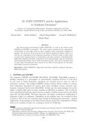
expensive operation. Fast Multipole Methods (FMM) have been used to reduce the<br />
number of calculations to O(N) [1,2,3]. These methods invoke Taylor expansions of<br />
forces due to multipole expansions of distant localized groups of particles. At large<br />
distances,target particles interact with collective sources,while at near distances,<br />
individual particle-particle interactions (
14<br />
has to communicate with a suitably defined neighborhood of “nearby” processors and<br />
involves the interchange of only a small number of particles close to the boundaries of<br />
the domains. However,in beam-beam calculations for circular colliders,this condition is<br />
violated,since the propagation of the particles through the external fields between beambeam<br />
interactions potentially causes them to wander over the entire spatial domain.<br />
Thus current parallel implementations of FMM are inadequate for such simulations.<br />
In this work we describe a very simple parallelization of a FMM based beam-beam<br />
interaction code. We continue to use a serial FMM algorithm,but embed it in a clever<br />
parallel communication scheme called Force Decomposition (FD) [5],initially developed<br />
for molecular dynamics simulations. Without the FMM,each processor in the FD<br />
algorithm would perform an N ′2 brute force calculation,where N ′ = N/ √ P ,with P<br />
the total number of processors used. By replacing this brute force computation with<br />
a serial FMM algorithm on each processor we reduce the computational complexity to<br />
O(N ′ )=O(N/ √ P ). The advantage of this combined FMM/FD parallel method is<br />
that it is extremely easy to implement. The FD method itself involves two basic MPI<br />
routines,each called twice per interaction,and basic FMM calculations are performed<br />
exactly as in a serial based FMM code,just now on a reduced set of source and target<br />
particles.<br />
This paper is organized as follows. In section 2 we discuss the beam-beam ring<br />
model. In section 3 we discuss the macro particle tracking method for the beambeam<br />
interaction,and in section 4 a serial implementation of the FMM for the beambeam<br />
kick calculations. In section 5 we discuss the parallel force decomposition (FD)<br />
communication scheme. In section 6 we discuss our parallelization of the previous serial<br />
code which we denote as FD/FMM. Finally in Section 7 we summarize our findings and<br />
indicate directions for future work to increase the order of this speedup.<br />
2. The ring model<br />
WeassumearingwithoneIPatθ = 0 and two counter-rotating bunches. In this work<br />
we only treat head-on collisions ,and the reference point at which the distribution is<br />
studied is directly before the IP (θ mod 2π =0 − ). In what follows we use the convention<br />
that if some parameter or dynamical variable X describes one beam,then X ∗ describes<br />
the other beam.<br />
Let ψ n (z) andψ ∗ n (z) (z := (q, p),q =(x, y),p =(p x,p y )) denote the normalized<br />
phase space densities of the beams at θ =0 − +2nπ. Then the representation of the one<br />
turn map for the unstarred beam from turn n to n +1is<br />
T [ψ ∗ n ]=A ◦ K[ψ∗ n ] (1)<br />
where A represents the lattice without the beam-beam and K[ψ] is the collective beambeam<br />
kick. In highly relativistic beams the beam-beam force for head-on bunch crossings<br />
with zero crossing angle is essentially transverse (the space charge forces within each
15<br />
bunch are negligible). In this approximation,the collective kick is given by<br />
(<br />
)<br />
∫<br />
q<br />
K[ψ](q, p) =<br />
,k[ψ](q) =ζ g(q − q ′ )ρ(q ′ ) dq ′ , (2)<br />
p + k[ψ](q)<br />
R 2<br />
( √x2 )<br />
where g = ∇G, G(q) =− 1 log + y<br />
2π 2 is the Green’s function, ζ is a strength<br />
parameter and ρ(q) = ∫ ψ(q, p) dp is the spatial density.<br />
R 2<br />
The particle trajectories are propagated turn by turn via<br />
z n+1 = T [ψ ∗ n](z n ) ,z ∗ n+1 = T ∗ [ψ n ](z ∗ n) (3)<br />
and since the maps are measure preserving,the densities evolve via<br />
ψ n+1 (z n+1 )=ψ n (z n ) ,ψ ∗ n+1 (z∗ n+1 )=ψ∗ n (z∗ n ) . (4)<br />
Note that the T and T ∗ are explicitly distinguished,allowing for different parameter sets<br />
describing the starred and the unstarred lattice. Equations (1-4) define a representation<br />
of the beam–beam Vlasov-Poisson system using maps.<br />
3. Macro particle tracking<br />
Macro Particle Tracking (see also [2]) is a method for computing time dependent phase<br />
space averages of f<br />
∫<br />
〈f〉 n := f(z)ψ n (z) dz, 〈f〉<br />
∫R ∗ n := f(z)ψn ∗ (z) dz, (5)<br />
4 R 4<br />
which can be evaluated as,for example,<br />
∫<br />
∫<br />
(<br />
〈f〉 n = f(z) ψ 0 M<br />
−1<br />
n (z)) dz = f (M n (z)) ψ 0 (z) dz, (6)<br />
R 4 R 4<br />
where M n := T [ψn−1 ∗ ] ◦ ...◦ T [ψ∗ 0 ] is the symplectic n-turn map containing successive<br />
collective kicks. Note that the beam-beam kick function can be written as such an<br />
average over the beam-beam kernel with q fixed, k[ψn](q) ∗ = ζ 〈g(q −·)〉 ∗ n. The<br />
macro particle concept enters through approximating the phase space integrals by finite<br />
sums over macro particle trajectories. A popular implementation for high dimensional<br />
problems is Monte Carlo macro particle tracking (MCMPT) where an initial ensemble<br />
of identical macro particles is generated randomly at positions z k according to the initial<br />
∑<br />
density ψ 0 . Then 〈f〉 n ≈ 1 N k f(M n(z k )). Of course,if we approximate the kicks in<br />
Eq. (2) by this method then we have approximate trajectories η k (n) ≈ M n (z k ). Thus<br />
our final approximation is<br />
〈f〉 n ≈ 1 ∑<br />
f(η k (n)) . (7)<br />
N<br />
k<br />
This will be our procedure in this report. A refined method which captures the behavior<br />
outside the beam core more accurately is weighted macro particle tracking (WMPT)<br />
[2]. Here we start with the initial densities ψ 0 and ψ ∗ 0 defined on an initial mesh {z k}<br />
and a quadrature formula with weights w k . Using WMPT to update the approximate<br />
trajectories η k (n),the final approximation becomes 〈f〉 n ≈ ∑ k f(η k(n))ψ 0 (z k )w k .
16<br />
These procedures use only forward tracking of particles and conservation of<br />
probability is guaranteed by construction. In contrast to methods with an explicit<br />
mesh (like PF in [2]),naive computation of the collective kick is an O(N 2 ) operation.<br />
The fast multipole method [1] reduces this to O(N),albeit with a large order constant.<br />
4. A serial implementation of FMM for the beam-beam kick<br />
The fast multipole method (FMM) [1] is a tree code that allows the computation of the<br />
collective force of an ensemble of N charges on themselves to a given accuracy δ with<br />
an operations count O(N) given that the distribution of the ensemble in configuration<br />
space is not too irregular. It employs the fact that the force on a particle due to a<br />
distant localized “clump” of charge can be given by a finite order multipole expansion<br />
up to precision δ.<br />
The FMM algorithm successively subdivides an outer rectangle in configuration<br />
space occupied by the ensemble until,on the finest level of subdivision,no more than a<br />
fixed number (typically 40) of particles are in each box. This leads to a tree structure<br />
of boxes containing boxes containing boxes and so on,until the boxes on the finest level<br />
finally contain a small number of particles. In the non-adaptive version of the scheme<br />
all boxes on the same level have the same number of child boxes. We use the adaptive<br />
version in which a box only branches into child boxes if the box itself still contains too<br />
many particles. In the upward traversal of the tree (fine → coarse levels) the algorithm<br />
first computes the multipole (long distance) expansions for all boxes on the finest level<br />
explicitly. The next step is to generate multipole expansions around the center of the<br />
parent boxes by translating their children’s expansions to the center and adding them<br />
up,see Fig.(1). This is repeated at every level so that in the end every box,at every<br />
level of mesh refinement,has its own long distance expansion.<br />
The downward traversal of the tree (coarse → fine levels) begins with boxes that<br />
are separated from one another by more than one box (i.e. at the 3-rd coarsest<br />
level). The potential inside a given box due to the sum of the multipole expansions<br />
of all well separated boxes is converted into a Taylor polynomial around the center<br />
of that box. Taylor series around the centers of the boxes in the next finer level are<br />
generated by shifting the Taylor polynomials of the parent boxes to the centers of their<br />
children (Fig.(1)) and adding the contributions of the multipole expansions from the<br />
well separated boxes (in the child level) which now show up at the boarder of the well<br />
separated parents. This procedure is iterated until the finest level. Finally,for each box<br />
on the finest level the forces on the particles are computed by evaluating the explicitly<br />
given derivative of its local Taylor polynomial at the position of the particle plus a small<br />
number of direct Coulomb terms.<br />
The 2-D adaptive routines (DAPIF2),used in our simulations,were supplied by<br />
Greengard. For more details see Greengard in [1].<br />
FMM was originally invented for dynamics such as space charge where the force of N<br />
particles on themselves is computed. The beam-beam effect on the other hand consists of
17<br />
S c<br />
S c<br />
S c<br />
S c<br />
S<br />
p<br />
T c<br />
T c<br />
T<br />
p<br />
T c<br />
T c<br />
Figure 1. Schematic representation of FMM algorithm (see text). Upward sweep<br />
through boxing structure tree (fine → coarse levels): Far field multipole expansions<br />
(MPE) of individual charges are summed and evaluated at the center of source-child<br />
boxes S c . The MPE of source-children boxes are summed and evaluated at the center<br />
of corresponding parent box S p . Downward sweep through tree (coarse → fine levels):<br />
The MPE of far sources are evaluated at the center of a target parent box T p as local<br />
Taylor expansions. These local Taylor expansions are shifted and evaluated at centers<br />
of target children boxes T c . At the finest level, forces can be computed on individual<br />
target particles.<br />
the collective interaction among two distinct counter-rotating bunches without taking<br />
into account the space charge forces inside each bunch. In other words one has to<br />
compute the forces on N particles of the unstarred bunch exerted by the N ∗ particles<br />
of the starred bunch, and then in addition the forces on N ∗ particles in the starred<br />
bunch due to the N particles in the unstarred bunch. Let us assume for simplicity<br />
that N = N ∗ . The forces can then be computed at 4 times the computational expense<br />
of the space charge force calculations inside a single bunch. First,the 2N particles<br />
of both beams are considered as one ensemble,with the charges of the starred bunch<br />
unchanged and the charges of the unstarred bunch set to zero. Then FMM computes<br />
the “space charge” force of the 2N particles (half of them being uncharged) at the 2N<br />
spatial coordinates. The kick proportional to the force is applied,however,only to the<br />
particles of the unstarred bunch. Then the charges of the unstarred particles are set<br />
back to their original values and the charges of the starred particles are set to zero.<br />
After having FMM compute the new “space charge” forces,the kicks are applied to<br />
the particles of the starred beam only. Thus FMM is called twice with twice as many<br />
particles.
18<br />
5. The parallel force decomposition algorithm<br />
In this section we discuss the Force Decomposition (FD) algorithm as originally<br />
envisioned for MD simulations. In the next section we discuss our adaption of the<br />
FD algorithm for the beam-beam kick calculations utilizing FMM.<br />
The Force Decomposition (FD) algorithm was developed in 1995 by Plimpton<br />
and Hendrickson [5] originally as a parallel method for matrix-matrix multiplication<br />
without All-to-All communications (e.g. as used in 2D parallel FFT algorithms when<br />
all processors must communicate with each other at the same time during the transpose<br />
operation). The authors realized that this communication scheme (described below)<br />
could be adapted to short range force molecular dynamics simulations where two-body<br />
(and higher multi-body and bonded) forces could be computed more efficiently,over<br />
that of the more conventional spatial decomposition algorithms,for particle numbers<br />
in the range of N ∼ 10 5 − 10 6 . In molecular dynamics (MD) simulations,the main<br />
computational task involves the calculation of the force on particle i due the rest of the<br />
N particles, F i = ∑ N<br />
j=1 F ij. A brute force serial calculation (which is to be avoided<br />
at all costs) would involve an O(N 2 ) double-do-loop calculation of the form:<br />
do i =1,N<br />
do j =1,N<br />
F i ← F i + F ij<br />
enddo<br />
enddo . (8)<br />
The so called Replicated Data (RD) algorithm reduces the order count by distributing<br />
the particles amongst the P processors. Thus the outermost (i) do-loop is distributed<br />
amongst the processors and each processor computes the forces on its own N/P particles<br />
and then updates the position and momentum of these particles. However,in order<br />
to perform the next calculation,all N updated particle positions would need to be<br />
communicated to all processors; a communication operation that scales as N. A<br />
measure of the scalability of an algorithm is isoscalability IS,which is the ratio of the<br />
communication cost to the computation cost. An ideal algorithm has IS =1,which<br />
indicates that larger problems can utilize larger resources in the most efficient manner,<br />
i.e. the communication and computation costs scale commensurately. Unfortunately,<br />
the RD algorithm has IS = P ,which implies that the efficiency of the algorithm<br />
decreases with the number of processors P ,since the communication cost scales as<br />
P times the computation cost.<br />
The most common parallel algorithm used in molecular dynamics force calculations<br />
is Spatial Decomposition (SD). In SD,the physical domain is divided amongst the P<br />
processors,with each processor responsible for the particles within its sub-volume. Thus,<br />
computation cost scales as the volume or V ∼ N/P. For problems with short range<br />
potentials which can be treated as negligible after some finite cutoff radius r c ,the<br />
communication cost scales as the area A = V 2/3 ∼ (N/P) 2/3 in the limit of large N/P.
19<br />
If each processor’s sub-volume is on the order of rc 3 ,communication takes place between<br />
the processor and its nearest neighbors across its boundary areas and the communication<br />
cost can approach N/P asymptotically for large N/P. Thus,theoretically IS → 1for<br />
SD,though there can be impediments to reaching this limit [5].<br />
Note that RD divides up the particles while SD divides up the physical domain.<br />
RD has the advantage of being geometry free,with ease of coding for any arbitrary<br />
dimension of the physical coordinates (i.e. z a 2D,3D,vector,etc ...),though with<br />
the marked disadvantage of poor scalability. The surface area to volume ratio of SD<br />
communications makes it worth the added effort of coding for particles sizes typically<br />
greater than 10 6 .<br />
Force Decomposition (FD) has an isoscalability that lies between RD and SD and<br />
has been shown by Plimpton and Hendrickson [5] to out perform SD in the realm<br />
of under 10 6 particles. As shown in Fig.(2),FD parallelizes the force matrix F ij by<br />
‘col particles’<br />
nmbr_rows = (15,15,14,14);<br />
j ncols = 14<br />
nmbr_cols = (15,15,14,14);<br />
15 15 14<br />
30 31 44 45 58<br />
1 15 16<br />
1<br />
15<br />
i<br />
nrows = 15<br />
‘row particles’<br />
15<br />
16<br />
30<br />
31<br />
(0,0) (0,1)<br />
(0,2)<br />
(0,3)<br />
15<br />
30<br />
44<br />
58<br />
F i<br />
= ∑F F i<br />
= F i<br />
= F<br />
, j ∑ F , j ∑ i , j<br />
F i i<br />
i<br />
= ∑ F i , j<br />
j=<br />
1<br />
j=<br />
16<br />
j=<br />
31<br />
j=<br />
(1,0) (1,1) (1,2)<br />
45 (1,3)<br />
i = {16,...,30} i = {16,...,30} i = {16,...,30} i = {16,...,30}<br />
14<br />
14<br />
44<br />
45<br />
58<br />
(2,0) (2,1)<br />
(2,2)<br />
(2,3)<br />
(3,0) (3,1)<br />
(3,2)<br />
(3,3)<br />
P(i,j) =<br />
{coords(1), coords(2)}<br />
Figure 2. Parallel force decomposition (FD) of force matrix F ij on a 2D processor<br />
grid. Each processor owns approximately O(N/ √ P ) i-particle indices and O(N/ √ P )<br />
j-particle indices. A given processor, e.g. P 12 computes the partial forces on all its<br />
i-particles (here 16 − 30) due to all its j-particles (here 31 − 44).<br />
creating a processor grid which is two dimensional regardless of the dimension of the<br />
coordinates z =(q, p). Each processor, P rc ,is responsible for approximately N/ √ P<br />
target or i-particles and N/ √ P source or j-particles and thus can locally compute the<br />
partial forces F i = ∑ N/ √ P<br />
j=1<br />
F ij ,<br />
do i =1,N/ √ P<br />
do j =1,N/ √ P<br />
F i ← F i + F ij<br />
enddo<br />
enddo . (9)
20<br />
Here the i and j are local indices in a given processor (Note: Fig.(2)-Fig.(4) are labeled<br />
with global indices). With the use of neighbor lists (as used in SD) to tag the O(N/P)<br />
non-zero interactions in F i ,the computation cost scales as O(N/P). Though the FD<br />
algorithm can be coded for a non-square number of processors,we discuss it here for<br />
a square number. The total number of particles N need not be a multiple of the the<br />
number of processors P ,as is illustrated in Fig.(2) (which uses N =58andP =16for<br />
ease of discussion).<br />
i<br />
16<br />
23<br />
24<br />
30<br />
j<br />
1 15 16 30 31 44 45 58<br />
j=<br />
31...44<br />
F i<br />
= ∑ F i F i<br />
= ∑ F i , j<br />
F i<br />
= ∑ F i , j<br />
F i<br />
= ∑ F i ,<br />
, j<br />
j=<br />
1...15<br />
i = {16,...,23}<br />
j=<br />
45...58<br />
j=<br />
31...44<br />
j=<br />
45...58<br />
j<br />
j=<br />
16...30<br />
j=<br />
1...15<br />
j=<br />
16...30<br />
i = {16,...,23} i = {24,...,30} i = {24,...,30}<br />
16<br />
19<br />
20<br />
i 23<br />
24<br />
27<br />
28<br />
30<br />
j<br />
1 15 16 30 31 44 45 58<br />
58<br />
58<br />
F i<br />
= ∑ F i , j F i<br />
= ∑ F i , j<br />
F i<br />
= ∑ F i , j F i<br />
= ∑ F i ,<br />
j=<br />
1<br />
j=<br />
1<br />
j=<br />
1<br />
i = {16,17,18,19} i = {20,21,22,23} i = {24,25,26,27}<br />
58<br />
58<br />
j=<br />
1<br />
i = {28,29,30}<br />
j<br />
Figure 3. Summation of total forces in a processor grid-rowby recursive halving(see<br />
text). Each processor obtains the total forces on approximately O(N/P) i-particles<br />
in log 2 (N/ √ P ) steps. (For processor P 12 these are i-particles {24, 25, 26, 27}). This<br />
operation is implemented via a call to MPI REDUCE SCATTERV.<br />
Within each row of the processor grid the goal is to obtain the total force ∑ N<br />
j=1 F ij<br />
for each of the N/ √ Pi-particles in that row. This is accomplished by the following clever<br />
recursive halving communication scheme,depicted in Fig.(3) for the second processor<br />
row of Fig.(2). At the first stage,each processor halves the number of partial forces it<br />
has for its i-particles and sends them to a target processor in the same grid-row (top<br />
half of Fig.(3)). At the same time this processor receives half of the target processor’s<br />
partial forces. For example,processor (1, 0) sends its partial forces for 24 ≤ i ≤ 30 to<br />
processor (1, 2) while receiving the partial forces for 16 ≤ i ≤ 30 from this processor.<br />
After this first stage,each processor in the grid-row now owns a more complete (yet<br />
not fully complete) set of partial forces,but now for only half of its original i-particles.<br />
This process is now repeated in log 2 (N/ √ P ) stages until each processor in the grid-row<br />
owns the total force ∑ N<br />
j=1 F ij,for N/P i-particles. The bottom half of Fig.(3) illustrates<br />
the second stage of this process. This recursive halving entails a communication cost<br />
that scales as O(N/ √ P ) and is accomplished in MPI by the call MPI REDUCE SCATTERV<br />
with an MPI SUM reduction operation. At this stage each processor updates its N/P<br />
coordinates for which it has the total forces ( i.e solve ẍ i = F i /m i ).
21<br />
i<br />
16<br />
j<br />
1 15 16 30 31 44 45 58<br />
n+<br />
1 n<br />
n+<br />
1 n n+<br />
1 n n+<br />
1 n<br />
z i<br />
zi<br />
z i<br />
zi<br />
z i<br />
zi<br />
z i<br />
zi<br />
i = {16,17,18,19} i = {20,21,22,23} i = {24,25,26,27} i = {28,29,30}<br />
30<br />
i<br />
16<br />
j<br />
1 15 16 30 31 44 45 58<br />
n+<br />
1<br />
z i<br />
i = {16, ,30}<br />
n+<br />
1<br />
z i<br />
i = {16, ,30}<br />
n+<br />
1<br />
z i<br />
i = {16, ,30}<br />
n+<br />
1<br />
z i<br />
i = {16, ,30}<br />
30<br />
Figure 4. Communication of updated particles positions in a processor grid-rowin<br />
log 2 (N/ √ P )stepsbyrecursive doubling (see text). This operation is implemented by<br />
acalltoMPI ALLGATHERV.<br />
To return the data to its initial configuration,in order to begin the next calculation,<br />
FD invokes a recursive doubling of the data within a processor grid-row,Fig.(4) (i.e.<br />
the opposite of the recursive halving operation described above). This operation is<br />
accomplished by MPI ALLGATHERV and upon its completion,each processor in the gridrow<br />
has the updated coordinates for all of its N/ √ Pi-particles.<br />
So far,the FD communication scheme has taken place only within processor gridrows,with<br />
no inter-grid-row communications. However,while the recursive doubling<br />
operation above has updated all the i-particle coordinates within a grid-row,each<br />
processor still requires the updated coordinates for its j-particles in order to begin<br />
the calculations of the partial forces anew. An inspection of Fig.(2) reveals that the<br />
transpose processor P cr (when we utilize a two-digit designation of the processors in a<br />
2D processor grid) has precisely the i-particles that processor P rc requires for use as<br />
its own j-particles. Thus,the last step in the FD communication scheme is for these<br />
two processors to perform a point-to-point communication (via MPI SENDRECEIVE) to<br />
swap copies of their respective i-particles. Upon completion of this operation,the data<br />
has now returned to its original form and we are ready to start a new partial force<br />
calculation,as in Fig.(2).<br />
Since the computation cost scales as O(N/P) and the communication cost scales<br />
as O(N/ √ P ),the FD algorithm has an IS = √ P ,which is intermediate between<br />
RD and SD. FD retains the ease of coding and the geometry features of RD with a<br />
intermediate isoscalability. As N/ √ P grows large,the double-do-loop in Eq.(9) grows<br />
prohibitively large enough to warrant a transition to the SD algorithm with a near<br />
optimal isoscalability. As stated earlier,Plimpton and Hendrickson [5] have shown that<br />
FD out performs SD in the particle range N ∼ 10 5 − 10 6 .
22<br />
6. Parallel force decomposition with serial fast multipole method<br />
Our simple parallelization scheme for the beam-beam interaction is now easily described.<br />
We employ a FD parallel communication strategy where the on-processor partial force<br />
computations in Eq.(9) are replaced by a serial FMM calculation. As pointed out earlier,<br />
in the beam-beam interaction the row i-particles and column j-particles in Fig.(2) are<br />
in separate beams,say the unstarred and starred beam,respectively. Thus,on each<br />
processor,we first compute the total force on the i-particles due to all the j-particles<br />
(using FMM) and secondly compute the total force on the j-particles due to all the<br />
i-particles (with a second call to FMM). Once the total force on all the i-particles are<br />
known we can apply the momentum kick to each of the i-particles and then apply the<br />
symplectic map to the next IP (and similarly for the j-particles in the starred beam).<br />
What differs from the FD algorithm as discussed in the previous section,is that each<br />
beam does not need the updated coordinates of the other beam. This means that we<br />
can drop the MPI_SENDRECEIVE between transpose processors. Instead,between each IP<br />
our algorithm utilizes the pair of routines MPI_REDUCE_SCATTERV and MPI_ALLGATHERV,<br />
(Fig.(3) and Fig.(4)) in each processor grid-row for the accumulation of forces for the i-<br />
particles,and then another pair of calls MPI_REDUCE_SCATTERV and MPI_ALLGATHERV in<br />
processor grid-columns for the accumulation of forces for the j-particles. We denote this<br />
parallelization method FD/FMM. While serial FMM reduces an O(N 2 ) computation to<br />
O(N),FD/FMM reduces an O((N/ √ P ) 2 ) computation to O(N/ √ P ),yielding a √ P<br />
speedup.<br />
As a proof of principal we have written a test code implementing FD/FMM which<br />
functions as follows:<br />
1) Every processor sets up the two lattice maps.<br />
2) Two Monte Carlo ensembles representing the 2 bunches are generated by computing<br />
2N times 4 independent Gaussian random variables in transverse phase space and distributing<br />
e.g. the unstarred particles along the rows and the starred particles along the<br />
columns of the processor grid.<br />
3) The collective beam-beam kicks,starred on unstarred,are computed using the<br />
FD/FMM approach along the columns and then along the rows. Here FMM is called<br />
once on 2N/ √ P particles in the row cycle and then once again on the 2N/ √ P in the<br />
column cycle.<br />
4) Each processor applies the single particle lattice maps A and A ∗ for its portion of the<br />
starred and unstarred particles.<br />
5) Repeat step 3) and 4) for as a given number of turns around the ring.<br />
In our simulations we have achieved the expected √ P speedup (defined as the ratio<br />
of serial to parallel execution time) for N up to 10 7 particles. In future work,we will<br />
incorporate the FD/FMM strategy into the WMPT code and do a detailed comparison<br />
with the serial version.
23<br />
7. Summary and outlook<br />
One of the main advantages of FD/FMM is its ease of coding. We were able to transform<br />
the serial FMM code to an FD/FMM code in a couple of days,with most of the work<br />
entailing the re-dimensioning of local arrays from N → N/ √ P .Onecanalsomakeuse<br />
of MPI’s Cartesian topology routines to create grid-row and grid-column communicators<br />
to facilitate scatter and gather operations in FD algorithm. In all,a total of four MPI<br />
communications calls need to be invoked while the original serial FMM code remains<br />
unaltered. The serial FMM code is called by each processor to accomplish the force<br />
calculation only for the i and j particles that it owns. This is embedded in the efficient<br />
parallel communication framework of FD to obtain the total beam-beam kick on each<br />
particle.<br />
FD/FMM is limited by its isoscalability, IS = √ P ,which results from its<br />
communication cost scaling as N/ √ P . This is inherent in the FD algorithm and so<br />
the maximum speedup of √ P we achieved cannot be transcended with this method. As<br />
pointed out earlier,conventional parallel FMM methods are extremely inefficient in the<br />
beam-beam interaction context considered here since the particles move substantially<br />
over the physical domain between interactions. Thus FD/FMM offers an easy way to<br />
achieve some degree of speed up and ability to utilize a larger number of particles with<br />
a minimal amount of coding effort. This work highlights the need for the development<br />
of parallel FMM based algorithms for beam-beam interaction codes that can transcend<br />
the current spatial decomposition limitations. This will be a focus of our future work.<br />
In addition we will explore the application of FD/FMM to the so-called hybrid FMM<br />
approach,[2,3]. This approach significantly reduces the number of points at which<br />
FMM has to compute the forces by laying down a PIC like grid and defining a minimum<br />
number, n,of particles per cell. Cells with more than n particles per cell are defined to<br />
be in the core and are deposited on the cell corners and the other cells are in the halo.<br />
The corners of the core cells and the halo particles are then fed to FMM.<br />
8. Acknowledgments<br />
We thank L. Greengard for supplying the adaptive FMM routines. Our work was<br />
supported by DOE grant DE-FG03-99ER41104. All simulations were performed at the<br />
Albuquerque High Performance Computing Center.<br />
References<br />
[1] L. Greengard, Thesis, The Rapid Evaluation of Potential Fields in Particle Systems, The MIT<br />
Press, Cambridge, MA (1988);<br />
L. Greengard, L. Rokhlin, A Fast Algorithm For Particle Simulations, Journal of <strong>Computational</strong><br />
<strong>Physics</strong> 73, 325-348 1987.<br />
[2] M.Vogt, T.Sen, J.A.Ellison, Simulations of Three 1-D Limits of the Strong-Strong <strong>Beam</strong>-<br />
<strong>Beam</strong> Interaction in Hadron Colliders Using Weighted Macro-Particle Tracking Phys. Rev.
24<br />
ST Accel. <strong>Beam</strong>s 5, 024401 (<strong>2002</strong>) and FNAL Pub-01/096-T (2001); M.Vogt, J.A.Ellison,<br />
T.Sen, R.L.Warnock, Two Methods for Simulating the Strong-Strong <strong>Beam</strong>-<strong>Beam</strong> Interaction<br />
in Hadron Colliders, Fermilab <strong>Beam</strong>-<strong>Beam</strong> Workshop (2001), Ed. T. Sen and M. Xiao,<br />
http://www-ap.fnal.gov/~meiqin/beambeam01/beambeam01.html.<br />
[3]F.W.Jones,Proc. Workshop on Space Charge <strong>Physics</strong> in High Intensity Hadron Rings, Ed.<br />
A. U. Luccio and W. T. Weng, AIP Conf. Proc. 448, (1998);<br />
W. Herr, M.-P. Zorzano and F. W. Jones, Phys. Rev. ST-AB 4 054402, (2001);<br />
W. Herr, M.-P. Zorzano and F. W. Jones, Fermilab <strong>Beam</strong>-<strong>Beam</strong> Workshop (2001), Ed. T. Sen<br />
and M. Xiao, http://www-ap.fnal.gov/~meiqin/beambeam01/beambeam01.html.<br />
[4] M.S. Warren and J.K. Salmon, A Portable Parallel Particle Program Computer <strong>Physics</strong><br />
Communication 87, 266-290 (1995); J.K. Salmon, M.S. Warren, and G.S. Winckelmans, Fast<br />
Parallel Tree Codes for Gravitational and Fluid Dynamical N-Body Problems, International<br />
Journal of Supercomputer Applications and High Performance Computing 8, 129-142 (1994).<br />
[5] S. Plimpton, Fast Parallel Algorithms for Short-Range Molecular Dynamics, J. Comp Phys.<br />
117, 1 (1995); B. Hendrickson and S. Plimpton Parallel Many-Body Simulations Without Allto-All<br />
Communications,Journal of Parallel and Distributed Computing, 27, 15-25 (1995); S.<br />
Plimpton and B. Hendrickson A New Parallel Method for Molecular Dynamics Simulation of<br />
Macromolecular Systems, J.Comp.Chem17, 326 (1996). Alsing, P.M., Kale, R.P., and Fleharty,<br />
M.E., Parallel Molecular Dynamics Visualization using MPI and MPE Graphics, Proceedings<br />
IEEE, Second MPI Developers Conference, Library of Congress #96-76653, 104 (July 1-2, 1996).
Inst. Phys. Conf. Ser. No 175<br />
Paper presented at 7th Int. Conf. <strong>Computational</strong> <strong>Accelerator</strong> <strong>Physics</strong>, Michigan, USA, 15–18 October <strong>2002</strong><br />
©2004 IOP Publishing Ltd<br />
25<br />
Accuracy analysis of a 2D Poisson-Vlasov PIC<br />
solver and estimates of the collisional effects in<br />
space charge dynamics<br />
A. Bazzani †, G. Turchetti ,<br />
C. Benedetti, A. Franchi, S. Rambaldi<br />
Dipartimento di Fisica Università di Bologna, INFN Sezione di Bologna, ITALY<br />
Abstract.<br />
We analyze the accuracy of a 2D Poisson-Vlasov PIC integrator, taking the KV<br />
as a reference solution for a FODO cell. The particles evolution is symplectic and<br />
the Poisson solver is based on FFT. The numerical error, evaluated by comparing the<br />
moments of the distribution and the electric field with the exact solution, shows a<br />
linear growth. This effect can be modeled by a white noise in the envelope equations<br />
for the KV beam. In order to investigate the collisional effects we have integrated the<br />
Hamilton’s equations for N charged macro-particles with a hard-core r H , reducing the<br />
computational complexity to N 3/2 . In the constant focusing case we observed that a<br />
KV beam, matched or mismatched relaxes to the Maxwell-Boltzmann self consistent<br />
distribution on a time interval, which depends on r H and has a finite limit for r H → 0.<br />
A fully 3D PIC code for short bunches was developed for the the ADS linac design<br />
at LNL (Italy). A 3D particle-core model, based on Langevin’s equations with the<br />
drift and noise terms given by Landau’s integrals, has been considered in viewof the<br />
inclusion of collisional effects in the the Poisson-Vlasov equation.<br />
1. Introduction<br />
High intensity linacs and storage rings are being considered for fundamental research on<br />
matter at very high energy density and a variety of applications ranging from neutron<br />
spallation sources to nuclear wastes transmutation and inertial fusion. In high intensity<br />
accelerators the major problems are the field quality and the control of small losses.<br />
In the storage rings,where the number of visited FODO cells can be as high as 10 6 ,<br />
the resonances between the collective motion of the core and nonlinear betatron motion<br />
may cause slow diffusion and affect the dynamic aperture. Moreover the collisional<br />
effects need to be considered because the changes induced in the distribution may be<br />
relevant on a long time scale. The semi-analytical tools available are mainly based on<br />
the particle-core models developed to study the behavior of a test particle in a given<br />
self consistent field of the core. The application of the frequency map analysis to these<br />
models allowed to detect the key role of the mismatch oscillations in the diffusion process<br />
which may explain the growth of the halo [1,2,3]. The analytical self consistent solutions<br />
of the 2D and 3D Poisson-Vlasov (P.V.) equation for the particles distribution and the<br />
corresponding electric field are confined to the constant focusing case [4],in which a a<br />
linear and nonlinear stability analysis of small perturbations have also been developed<br />
[5,13]. The excitation of the lowest unstable mode was proposed as a possible escape<br />
mechanism from the core,generating the halo [6,7]. For the periodic focusing case<br />
† To whom correspondence should be addressed: bazzani@bo.infn.it
26<br />
numerical PIC solutions are extensively used since the only known analytic solution<br />
is KV distribution in the 2D case. We have developed a 2D PIC code for a lattice<br />
of identical FODO cells in order investigate its convergence properties,the onset of<br />
instabilities and the dynamics of test particles. This program has been undertaken using<br />
the KV as a reference solution in the periodic focusing case. Our 2D PIC solver is based<br />
on a symplectic integrator and a FFT Poisson solver which allows to impose Dirichelet<br />
conditions on a arbitrary closed boundary. For a matched KV solution the error on the<br />
electric field and on the moments of the distribution are analyzed as a function of the<br />
number K of Fourier components in each dimension and the number of pseudo-particles<br />
N. In this case the rms radii,the emittance and the field error exhibit a linear growth.<br />
For a fixed K we observe a decrease with N with a possible asymptotic limit; for K<br />
fixed the error decreases reaches a minimum and increases again. The linear growth<br />
of the moments is related to the accumulation numerical errors ( due to the grid size<br />
and to the density fluctuations),which behave as a noise in the equations of motion[10];<br />
For a circular machine to keep the error growth sufficiently small is a computational<br />
challenge¿ In this case the effect of Coulomb collisions cannot be neglected. To this<br />
end we have developed a molecular dynamics algorithm to integrate symplectically a<br />
system of N macro-particles,reducing the computational complexity from N 2 to N 3/2<br />
(with a multipolar expansion of the far field). We have introduced a hard core r H so<br />
that an elastic collision occurs whenever there is a contact. In the absence of hard core<br />
the close encounters are resolved by increasing the integration accuracy. It is found<br />
that an initial KV distribution evolves towards the self consistent Maxwell-Boltzmann<br />
distribution. This relaxation process cannot be obtained within the framework of a mean<br />
field equation like P.V. The relaxation time increases as r H decreases and has a finite<br />
limit for r H → 0. An estimate of the relaxation time for the lattice of identical FODO<br />
cells previously considered is given. We have also developed a fully 3D parallel PIC<br />
code in order in order to study the evolution of a bunch in the linac ISCL,a project of<br />
the INFN laboratories of Legnaro (Italy).. In that case a Neuffer-KV initial distribution<br />
evolves numerically,with our PIC solver,towards a Fermi-Dirac distribution whose<br />
tails are Maxwellian. [11] We present a 3D particle core model defined by a Langevin<br />
equation with a drift and noise given by the Landau integrals in view of an inclusion of<br />
the collisions in the PIC code as recently proposed [12].<br />
The plan of the paper is the following: we describe our 2D model in section 2,the<br />
PIC solver in section 3,we present the error analysis in section 4,the related Langevin<br />
model in section 5,we analyze the MD approach to collisions in section 6,3D extensions<br />
and the related particle-core Langevin model in section 7.<br />
2. The model<br />
2.1. The Hamiltonian<br />
We consider a coasting beam on a lattice of identical FODO cells of length L at the end<br />
of which a thin sextupole can be switched on. The Hamiltonian is<br />
H ph = p2 xph + p2 yph<br />
2<br />
+ k0,x(s ph<br />
ph ) x2 ph<br />
2 − kph 0,y(s ph ) y2 ph<br />
2 +<br />
+ K 2,ph<br />
6 (x3 ph − 3x ph y 2 ph)δ L (s ph )+ ξ ph<br />
2 V ph(x ph ,y ph )<br />
(1)
27<br />
where K 2,ph is the sextupolar gradient, δ L denotes the periodic Dirac function of period<br />
L, ξ ph is the perveance defined by<br />
ξ ph =<br />
2qQ<br />
p 0 v 0 γ = 2qI<br />
(2)<br />
2 mc 3 β 3 γ 3<br />
and I is the current, Q the total charge per unit length. In order to use dimensionless<br />
variables we scale the longitudinal coordinates with L the transverse ones with a. Asa<br />
consequence dropping the label ph on the scaled variables we have x ph = ax, s ph = Ls,<br />
p x,ph = p x a/L and L 2 k ph<br />
0,x = k 0,x , aLK 2,ph = K 2 and ξ ph L 2 /a 2 = ξ. Finally letting<br />
H ph = a 2 L −2 H and V ph (x ph ,y ph )=V (x, y) the scaled Hamiltonian reads<br />
H = p2 x + p2 y<br />
+ k 0,x (s) x2<br />
2<br />
2 − k 0,y(s) y2<br />
2 + K 2<br />
6 (x3 − 3xy 2 )δ(s)+ ξ V (x, y) (3)<br />
2<br />
The self consistent potential satisfies the Poisson equation<br />
∫<br />
∆V = −4πρ S (x, y, s) ρ S (x, y, s) = ρ(x, y, p x ,p y ,s)dp x dp y (4)<br />
where ρ is the solution of the Liouville equation for the Hamiltonian H namely<br />
∂ρ<br />
+[ρ, H] =0 (5)<br />
∂t<br />
We remark that the emittances scale as well according to ɛ ph = ɛa 2 /L. Correspondingly<br />
the optical functions and the corresponding amplitudes scale according to β x,ph = Lβ x<br />
and A x,ph = √ ɛ x,ph β x,ph = aA x . The advantage of this choice is that all the quantities<br />
become of order 1 choosing a of the order of the transverse size of the beam.<br />
2.2. The FODO cell<br />
It has a unit length,the quadrupoles length is 0.2 and their gradients are k 0,x = k 0,y =<br />
12,the emittances are ɛ x = ɛ y = 1 (tipically L =1m,a = 1 mm). The perveance<br />
range we considered is [1, 10],the results presented refer to ξ = 10 for which the tune<br />
depressions 0.1.<br />
2.3. Envelope equation<br />
In order to analyze the performance of the PIC solver for equations (4) and (5) we<br />
consider first a linear lattice (K 2 = 0) and K.V. beam whose phase space distribution is<br />
ρ = 1 δ ( 1 − X2 + Px<br />
2 + Y 2 + P 2 )<br />
y<br />
π 2 ɛ x ɛ y ɛ x ɛ y<br />
ρ S =<br />
1<br />
πA x A y<br />
ϑ ( 1 − x2<br />
A 2 x<br />
− y2 )<br />
A 2 y<br />
where the normalized coordinates are given by X = xβx −1/2 , P x =(α x x + β x p x )βx<br />
−1/2<br />
and the optical functions are related by β x = A 2 x /ɛ x, α x = −A x A ′ x /ɛ x to the amplitudes<br />
A x,y which are the periodic solutions (matched beam) of the envelope equations<br />
d 2 A x<br />
ds 2<br />
− ɛ2 x<br />
+ k<br />
A 3 0,x A x =<br />
x<br />
3. The PIC solver<br />
2ξ<br />
A x + A y<br />
d 2 A y<br />
ds 2<br />
(6)<br />
− ɛ2 y<br />
2ξ<br />
+ k<br />
A 3 0,y A y =<br />
(7)<br />
y<br />
A x + A y<br />
The numerical solution of Poisson-Vlavov equations was obtained with a PIC code by<br />
using N pseudo-particles. A parallel version for the evolution has been developed with<br />
MPI.
28<br />
3.1. Initial distribution<br />
We first change to the linearly normalized coordinate and perform the following<br />
transformation<br />
X = √ √<br />
tuɛ x cos(2πφ x ) Y = t(1 − u)ɛ y cos(2πφ y ) (8)<br />
P x = √ √<br />
tuɛ x sin(2πφ x ) P y = t(1 − u)ɛ y sin(2πφ y ) (9)<br />
where t ≥ 0andu, φ x ,φ y ∈ [0, 1]. The following relation holds<br />
ρ(X, P x ,Y,P y )dX, dP x dY dP y = ρ(t, u, φ x ,φ y )π 2 ɛ x ɛ y tdtdφ x dφ y du (10)<br />
For the case of a K.V. distribution we have ρ =(π 2 ɛ x ɛ y ) −1 δ(1−t) and the distribution is<br />
obtained by fixing t = 1 and filling uniformly the unit hypecube [0, 1] 3 in the (u, φ x ,φ y )<br />
space. The waterbag distribution for which ρ =(π 2 ɛ x ɛ y ) −1 2θ(1−t) is obtained by filling<br />
uniformly the unit hypercube [0, 1] 4 in the (t 2 ,u,φ x ,φ y ) space.<br />
3.2. The evolution scheme<br />
We have considered a second order symplectic evolution scheme . The Hamiltonian (3)<br />
can be written as H = H 0 + H sex + 1 ξV and the numerical scheme consists in replacing<br />
2<br />
the space charge contribution in each interval s i+1 − s i with an impulsive force at s i<br />
(kick approximation),whereas the linear evolution from s i to s i+1 due to H 0 is computed<br />
exactly. The sextupole contribution ,if any,is also a kick.<br />
3.3. The Poisson solver<br />
The Poisson equation is solved by a spectral method. We choose a rectangle |x| ≤<br />
1<br />
Λ 2 x, |y| ≤ 1Λ 2 y whose sides are at least 3 times bigger than the amplitudes A x ,A y .<br />
We consider a grid whose cells have sides ∆x =Λ x /K x , ∆y =Λ y /K y where K x ,K y<br />
are powers of 2 and at any grid point we compute the density either by the nearest<br />
grid points (NPG) deposition method or by the cloud in cell (CIC) deposition method.<br />
The potential is obtained by a FFT transform and the electric field is computed by a<br />
centered difference. To speed up the computation one FFT may be replaced by the<br />
solution of a three diagonal system which reduces the computational complexity from<br />
(K log K) 2 to K 2 log K. The potential is computed by imposing Dirichelet conditions<br />
V = 0 at the boundary of the square; these conditions can be imposed on an arbitrary<br />
closed curve,by using a Green’s function method which doubles the computation time<br />
at each step once a K × K matrix is inverted,for an approximation of the given curve<br />
with a polygonal with K vertices.<br />
4. Error analysis<br />
A rigorous analysis of the discretization error introduced by a PIC code with respect<br />
to the exact solution is a very hard task. We remark that the approximate solutions<br />
depend on the box size Λ,(assuming Λ x =Λ y = Λ),on the the number K of Fourier<br />
components (assuming K x = K y ) which fixes the space resolution ∆x =Λ/K,on the<br />
particle number N andontheintegrationstep∆s. The exact result is recovered in<br />
the limit Λ →∞, ∆s → 0andK, N →∞,once this limit is correctly defined. We<br />
have fixed the first two parameters by choosing ∆s =1/100 (this is the average of ∆s i )<br />
and Λ = 20 so that for the chosen value of the perveance ξ = 10 it is larger than 3
29<br />
Log ε<br />
Log K<br />
K=32<br />
K=64<br />
K=128<br />
K=256<br />
Log N<br />
Log N<br />
Figure 1. Sketch of the dependence of the error on K and N (left). Sketch of<br />
the behavior of K opt as a function of N and corresponding power law K opt = CN β<br />
continuous interpolation.<br />
times the amplitudes. The error introduced by the longitudinal step is of order (∆s) 2<br />
and we checked this is the case on the solution of envelope equation we computed by<br />
integrating (7) with the same procedure (splitting method with exact integration of the<br />
linear part and kicks for the space charge force). The error dependence on K and N has<br />
been examined. We investigate the double limit by letting first N →∞and considering<br />
the its dependence on K. Indeed N can be increased up to 10 6 and occasionally 10 7 ,<br />
whereas K is limited to a few values ranging from 32 to 512. We have checked that by<br />
increasing N the error decreases up to a limit value,which can be further reduced by<br />
increasing K. As consequence if we fix N and vary K,the error first decreases reaches<br />
a minimum and then increases. The error we consider refers to the electric field and to<br />
the moments of the distribution. Since the error growth with s is linear,see figures 2<br />
and 3,we have computed the slope and studied its dependence on N and K. Forfixed<br />
K the slope appears to follow a power law N −α with an exponent α slightly smaller<br />
than 1 before the asymptotic region is reached; the asymptotic limit decreases with K.<br />
Fixing N at a low value the error increases with K. As a consequence for fixed N the<br />
error decreases,reaches a minimum and then increases again,as shown qualitatively by<br />
figure 1. The optimal value of K is a stepwise function of N for which we propose a<br />
power law interpolation K = cN β .<br />
4.1. Scaling law<br />
A power law is found if we assume that the optimal condition is reached when the<br />
relative error on the density,given by the statistical fluctuation,is equal to uncertainty<br />
in the space resolution. Denoting by n P<br />
the average number of particles per cell in<br />
thecoreandbyl the core diameter such condition is ∆n P<br />
/n P<br />
≃ ∆x/l. Letting η the<br />
fraction of the box occupied by the core,the diameter of the core is given by l ≃ η 1/2 Λ.<br />
The side of the cell is ∆x =Λ/K so that the uncertainty in the position within the core<br />
is ∆x/l =1/(Kη 1/2 ) For a uniform distribution the number of occupied cells is ηK 2<br />
and the average number of particles per cell is n P<br />
= N/(ηK 2 ). As a consequence since<br />
the statistical fluctuation is ∆n P<br />
= √ n P<br />
by equating the position uncertainty to the<br />
cell population uncertainty n −1/2 =∆x/l we obtain<br />
P<br />
N ≃ η 2 K 4 (11)
30<br />
2<br />
2<br />
2<br />
ε<br />
ε<br />
ε<br />
1<br />
0 s<br />
1000<br />
1<br />
0 s<br />
1000<br />
1<br />
0 s<br />
1000<br />
Figure 2. Variation of the emittances ɛ x , ɛ y with the iteration number n for different<br />
values of the number of Fourier components K = 64 (left frame), K = 128 (central<br />
frame), K = 256 (right frame). In each frame the x and y emittancehavethesame<br />
color which changes with the particles number: N =10 3 (light blue), N =2.510 3<br />
(red), N =510 3 (blue), N =10 4 (green), N =10 5 (purple).<br />
4.2. Numerical experiments<br />
We have analyzed the error dependence on K and N on a model of FODO cell with a<br />
high value of the perveance. This choice was made since we observed that the behavior<br />
of the error was clearly detectable for a moderate number of iterations s max =10 3 .<br />
Indeed the most relevant effect of discretization is a numerical noise which causes a<br />
linear growth of the moments of the distributions and of the error in the electric field.<br />
The growth rate increases with the perveance. We consider the FODO cell of section<br />
2withaperveanceξ = 10. The bare and depressed tune are ν 0 x = ν 0 y =61.8 o and<br />
ν x = ν y =6.5 o ,the bare amplitudes A 0 x =1.21, A 0 y =0.81,the core amplitudes<br />
A x =3.65, A y =2.53. The number of longitudinal steps per FODO cell used is 100,<br />
the periodic solution is found by a Newton’s method and the accuracy of the symplectic<br />
integration procedure agrees with the theoretical estimate (∆s) 2 =10 −4 . The size of<br />
the square where Poisson equation is solved is Λ = 20 so that fraction occupied by the<br />
core is η =0.07. The relative error on the electric field is defined by<br />
( ∫<br />
∆E<br />
E = D ∗<br />
[(E x − E xex ) 2 +(E y − E yex ) 2 ] dx dy ) 1/2<br />
( ∫ (12)<br />
D ∗<br />
[Exex 2 + E2 yex ] dx dy) 1/2<br />
where the integrals are extended to the D ∗ =[−2.5, 2.5] 2 a domain almost entirely within<br />
the core. In this way we can ignore errors due to the non-zero field on the boundaries.<br />
In figure 2 we show the variation of the emittances defined by ɛ x =4(<br />
− 2 ) 1/2 ,with the number s of visited FODO cells. It is evident that the growth<br />
is linear with s and that the slope decreases with N. WhenK increases for a fixed N,<br />
the slope also increases,except for for the highest value N =10 5 ,shown in figures 2,<br />
for which the minimum occurs at K = 128. In figure 3 we consider the variation of<br />
the error in the electric field ∆E/E with the iteration number s. We observe that the<br />
error growth with s is still linear and that the slope decreases with N for a fixed K. We<br />
have also fitted a line a + bn to the error growth in order to examine the dependence<br />
of the coefficient b on N and K. The scaling law suggests that increasing K by 2 the<br />
optimum N should increase by 2 4 ,a result compatible with our numerical observations.<br />
For K =64theoptimumN is below 10 5 a value above which the error does not decrease
31<br />
0.3<br />
0.3<br />
0.3<br />
δΕ/Ε<br />
δ Ε/Ε<br />
δΕ/Ε<br />
0<br />
0 s<br />
1000<br />
0<br />
0 s<br />
1000<br />
0<br />
0 s<br />
1000<br />
Figure 3. Variation of error on the electric field δE/E with the iteration number s<br />
for different values of the number of Fourier components K = 64 (left frame), K = 128<br />
(central frame), K = 256 (right frame). In each frame the color which changes with<br />
the particles number: N =10 3 (light blue), N =2.510 3 (red), N =510 3 (blue),<br />
N =10 4 (green), N =10 5 (purple).<br />
-2<br />
k= 64<br />
-2<br />
k= 128<br />
-2<br />
Log __ dε<br />
dn<br />
Log __ dε<br />
dn<br />
Log __ dε<br />
dn<br />
-6<br />
3 Log N<br />
6<br />
-6<br />
3 Log N<br />
6<br />
-5<br />
0 Log ξ<br />
2<br />
Figure 4. Variation of the slope b of the emittance ɛ x = a + bs, determined by least<br />
square fit, with respect to N, for different values of the number of Fourier components:<br />
K = 64 (left frame),K = 128 (central frame) . Variation of the slope with the perveance<br />
ξ forN =10 4 and k = 128 (right frame).<br />
appreciably. This is shown by figure 4 where dependence of the emittance slope on N<br />
is shown for a fixed value of K. The saturation for K = 64 is evident,whereas it is<br />
not reached for K = 128 up to N =10 6 . In the same figure we show the variation of<br />
the slope with the perveance which is monotonic and approximately given by b ∝ ξ 3/2 .<br />
The results described above refer to the NPG deposition method. We have repeated the<br />
same simulations with CIC deposition method and the difference was typically within<br />
10%,without any significant variation for the dependence on K and N described above.<br />
5. The Langevin equation<br />
We consider a stochastic model suitable to describe the linear rise of the errors with<br />
number of visited cells s. We assume that the fluctuations in the particle number in every<br />
cell is equivalent to a white noise in the equations of motion. This is by no means related<br />
to the physical collisions which preserve asymptotically the kinetic energy. Referring
32<br />
still to a KV beam the equations of motion become<br />
d 2 x<br />
ds + k 2 x x = η dw<br />
d 2 y<br />
ds<br />
ds + k 2 y x = η dw<br />
(13)<br />
ds<br />
where w(s) denotes a Wiener process and the the depressed gradients k x ,k y are defined<br />
by k x (s) =k 0 x − 2ξ ( A x (A x + A y )) −1 and similarly for k y . The amplitudes A x and A y<br />
are solutions of the envelope equation<br />
d 2 A x<br />
ds 2<br />
− ɛ2 x<br />
+ k<br />
A 3 x (s)A x =0<br />
x<br />
We recall that when η = 0 the following relations hold<br />
= A2 x<br />
4<br />
d 2 A y<br />
ds 2<br />
− ɛ2 y<br />
+ k<br />
A 3 y (s)A y = 0 (14)<br />
y<br />
= 1 ɛ 2 x<br />
+ 1( dA ) x 2<br />
= 1<br />
x 4 ds<br />
4 A dA x<br />
x<br />
ds (15)<br />
By taking the average also on the stochastic process we find that the second moments<br />
grow linearly with s with a slope proportional to η 2 .<br />
This can be easily proven by direct computation in the smooth focusing<br />
approximation and zero space charge limit. In the symmetric case k 0,x (s) =k 0,y (s)<br />
are replaced by a constant ω0 2 and the fluctuations change the x and y emittance ɛ 0<br />
into ɛ(s) = ɛ 0 +2η 2 s/ω 0 if one neglects oscillating terms. As a consequence since<br />
A 2 = ɛ(s)/ω 0 we see that dɛ 2 /ds =4ɛη 2 /ω 0 =4η 2 A 2 . More generally the amplitudes<br />
and the emittances satisfy the system of equations (14),where k x ,k y are replaced by<br />
ω0 2 and<br />
dɛ 2 x<br />
ds =4η2 A 2 dɛ 2 y<br />
x<br />
ds =4η2 A 2 y (16)<br />
Assuming these equations still hold in presence of space charge,one one has to replace<br />
k x (s), k y (s) withω 2 (s) =ω0 2 − ξ/A 2 (s). In order to find an approximate solution for a<br />
matched beam we observe that the numerical solution shows that A(s) varies slowly so<br />
that in (16) one can replace A 2 (s) withA 2 (0) = ɛ 0 /ω(0) namely<br />
ɛ(s) = ( ɛ 2 0 +4ɛ 0<br />
η 2 s ) 1/2<br />
≃ ɛ0 +2 η2 s<br />
ω(0)<br />
ω(0)<br />
In (17) the linear approximation holds for 4η 2 s/ɛ 0 ω(0) ≪ 1andω(0) = ɛ 0 /A 2 (0) where<br />
A 2 (s) =<br />
ξ + ɛ(s) ( ξ 2 ) 1/2<br />
1+ (18)<br />
2ω0<br />
2 ω 0 4ɛ 2 (s)ω0<br />
2<br />
The errors on the emittance and the amplitude are given by (17) and (18) whereas for<br />
the electric field we have E = x ξ/A 2 (s) and the error is computed according to (12).<br />
The result for ξ ≫ 1 simplifies and setting γ =2η 2 /ω(0) we have<br />
ɛ(s) =ɛ(0) + γs A 2 (s) =A(0) 2 + γ<br />
ξA(0) s<br />
(17)<br />
δE ∣ ∣∣1<br />
E = A 2 (s)<br />
−<br />
A 2 ∣ =<br />
2γ<br />
(0) ξA 2 (0) s (19)<br />
In our model using the smooth focusing approximations we obtain A =2.95,to be<br />
compared with the average of the amplitude over one period =< A y >=3.08.<br />
The estimate of the slope for the electric field error growth is 0.022 times the slope of the<br />
emittance growth; fitting that data of our simulations we find a range of values between<br />
0.018 and 0.03 which is compatible with the estimate.
33<br />
1.5<br />
1.5<br />
18<br />
ρ (E)<br />
ρ (E)<br />
χ 2<br />
0<br />
0 2.4<br />
E<br />
0<br />
0 E<br />
2.4<br />
0<br />
0 s<br />
6000<br />
Figure 5. Energy density for particles without hard core at s = 0 (left) and s = 6000<br />
(center). The red curve is the self consistent Maxwell-Boltzmann (MB) distribution.<br />
Right frame: The χ 2 for the discrepancy of the phase distribution ρ with respect to<br />
the MB distribution.<br />
6. Coulomb oscillators<br />
In order to estimate the effect of collisions we have developed a 2D molecular dynamics<br />
(MD) code. In this preliminary stage the smooth focusing approximation was chosen<br />
because the thermodynamic equilibrium distribution is known. The equations of motion<br />
for a system of N Coulomb oscillators are<br />
d 2 x i<br />
ds 2<br />
+ ω2 0 x i = ξ N<br />
∑<br />
j≠i<br />
x i − x j<br />
r 2 ij<br />
d 2 y i<br />
ds 2<br />
+ ω2 0 y i = ξ N<br />
∑<br />
j≠i<br />
y i − y j<br />
r 2 ij<br />
and we integrate them with a second order symplectic integrator. A more accurate<br />
integration is reserved to the subset of colliding particles (whose distances r ij are below<br />
an assigned value λ coll smaller than the average distance N −1/2 which in turn is smaller<br />
than the Debye radius,which for ξ ∼ 1is1/3 the beam size.<br />
R 2 = k T B<br />
= A2 〈p 2 x + p 2 〉 ( )<br />
y A 2<br />
2 ωɛ 0<br />
D = (21)<br />
4πq 2 ρ s 2ξ 2 4 ξ<br />
We have also considered a model in which the macro-particles have a hard core r H<br />
,so<br />
that elastic collisions occur when r ij =2r H<br />
. These collisions are treated with compiling<br />
a list for each step and linearly interpolating the elastically colliding particles. The<br />
simulations refer to a unit cells with bare phase advance ω 0 = 1 emittances ɛ 0 =2<br />
and perveance ξ =2sothatω =0.64. The second order moments,for a matched<br />
initial K.V. distribution,remains constant within the statistical error. The distribution<br />
changes and evolves to a Maxwell-Boltzmann self consistent distribution ρ = Z −1 e −H/kT<br />
where H = 1 2 (p2 + ω0 2r2 )+ ξ V (r) andV is the self consistent potential. The relaxation<br />
2<br />
time depends on the hard core radius and reaches a finite limit for r H<br />
→ 0. In figure<br />
5a and 5b we show the initial and final distribution in energy,when the equilibrium<br />
condition has been reached. The result is the same for any value of the hard core. In<br />
figure 5c we show instead the evolution of the distance from the equilibrium distribution,<br />
measured by the χ 2 (averaged on a small time interval to reduce the fluctuation). The<br />
hard core accelerates the relaxation process as expected and the dependence of the<br />
relaxation time on r H<br />
is smooth.<br />
(20)
34<br />
7. 3D model and its applications<br />
7.1. Scaling law for the PIC solver<br />
An analogous error analysis of our 3D PIC solver is a more difficult task. In the periodic<br />
focusing a self-consistent analytic solution of the Vlasov problem to be used as reference<br />
solution is not available. The coupling between longitudinal and transverse dynamics<br />
may also produce a fast relaxation of the bunch into a stationary distribution. Looking at<br />
the emittance behavior it is therefore difficult to distinguish the physical and numerical<br />
effects. A generalization of the scaling law given in sec. 4.1 reads<br />
N ≃ η 5/3 K 5 (22)<br />
where η is the fraction of the cube occupied by the core. With the parameters of the<br />
TRASCO-ISCL linac [8],a first set of simulations has been recently carried out [9].<br />
7.2. Collisional Particle in Core model<br />
The collisional effects within the Debye radius are modeled by using the Landau<br />
approach: the collisions are supposed to be ’soft’,binary and of short range. We<br />
introduce the drift and the diffusion coefficients<br />
a i (x,s)=η 2 ∂ρ 1<br />
D ik (x,s)= η2 ∂ 2 ρ −1<br />
(23)<br />
∂p i<br />
2 ∂p i ∂p k<br />
where ρ n (x,s) are the Rosenbluth potentials obtained by integrating the phase space<br />
density over a Debye sphere of center x,whose volume is V D<br />
∫ ρD (p ′ , x)<br />
ρ n (p, x,s)=<br />
‖p − p ′ ‖ n dp′ ρ D (p ′ , x,s)= 1 ∫<br />
ρ(x ′ , p,s) dx ′ (24)<br />
V D ‖x−x ′ ‖
35<br />
X 2<br />
1.2<br />
1<br />
0.8<br />
0.6<br />
0.4<br />
0.2<br />
0<br />
0 0.2 0.4 0.6 0.8 1 1.2<br />
X 1<br />
No. of particles<br />
12000<br />
10000<br />
8000<br />
6000<br />
4000<br />
2000<br />
0<br />
0.6 0.8 1 1.2 1.4<br />
energy<br />
Figure 6. Formation of a halo in due to the collision terms (left). Spread of the<br />
energy after a 500 FODO cells (right) for the matched (red) and mismatched (blue)<br />
case.<br />
where a i are the bunch amplitudes.<br />
We recall that the Particle in Core model is able to reproduce the single particle<br />
instabilities,but unable to observe the collective instabilities since its space charge field is<br />
not self consistent. On the contrary the PIC model is self consistent but is not optimized<br />
for the single particle instabilities,since the single particle contributes are averaged on<br />
the grid points. All these problems could be avoided by using a fully 3D Molecular<br />
Dynamics model,whose computational complexity is too high to be implemented with<br />
enough resolution.<br />
8. References<br />
[1] M. Lagniel Necl. Instr. Meth. A 345 (1994) 405.<br />
[2] A. Bazzani, M. Communian, A. Pisent Part. Accel. 63 (1999) 79.<br />
[3] M. Communian, A. Pisent, A. Bazzani, S. Rambaldi, G. Turchetti Phys. Rev. Special Topics -<br />
<strong>Accelerator</strong>s and <strong>Beam</strong>s Vol. 4, 124201 (2001)<br />
[4] R. L. Gluckstern, A. V. Fedotov, S. Kurennoy, R, Ryne Phys. Rev. 58, 4977 (1998)<br />
[5] I.Hofmann,Phys.Rev.E57 (1998) 4713.<br />
[6] R.L.GlucksternPhys.Rev.Letters73, 1247 (1994)<br />
[7] R. L. Gluckstern, W. H. Cheng, S. S. Kurennoy, H. Ye Phys. Rev E 54, 6788 (1996)<br />
[8] http://trasco.lnl.infn.it<br />
[9] A. Franchi et al. , LINAC conference, Korea <strong>2002</strong><br />
[10] J. Struckmeier, Phys. Rev. E54, 830 (1996)<br />
[11] G. Turchetti, S. Rambaldi, A. Bazzani, M. Communian, A. Pisent 3D solutions of the Poisson-<br />
Vlasov equations for a charged plasma and particle core model in a line of FODO cells - EPJ<br />
submitted (<strong>2002</strong>)<br />
[12] Ji Qiang, R. D. Ryne, S. Habib Self-consistent Langevin simulation of Coulomb collisions<br />
in charged particle beams technical paper, SC2000 conference, Dallas (2000)<br />
http://www.SC2000.org/proceedings/techpapr/papers/pap224.pdf<br />
[13] R. Davidson Phys. Rev. Letters 81, 991 (1998)
Inst. Phys. Conf. Ser. No 175<br />
Paper presented at 7th Int. Conf. <strong>Computational</strong> Accelarator <strong>Physics</strong>, Michigan, USA, 15–18 October <strong>2002</strong><br />
©2004 IOP Publishing Ltd<br />
37<br />
The COSY language independent architecture: porting<br />
COSY source files<br />
L. M. ChapinÝ, J.Hoefkensݧ and M. BerzÝ<br />
Ý Department of <strong>Physics</strong> and Astronomy, Michigan State University, East Lansing, MI 48824,<br />
USA<br />
Abstract. As part of the project of porting the code COSY INFINITY[1] to a language<br />
independent architecture, a tool is being developed that translates COSY language to C++<br />
language. The tool will allow the use of C++ classes for all elementary operations of COSY,<br />
which represent a wrapper around high-performance COSY C source. This will allow those<br />
unfamiliar with the COSY language access to the power of COSY.<br />
1. The COSY language independent architecture and the COSY syntax<br />
Recently the COSY system [1, 2, 3, 4, 5, 6] has been ported to a language independent<br />
platform to accommodate the use in various modern and widely used programming<br />
environments. In particular, the languages supported include FORTRAN 77, C, as well as the<br />
object oriented environments of FORTRAN 90 and C++. This is achieved in the following<br />
way. The original FORTRAN 77 based language environment consists mainly of operations<br />
on a suite of COSY objects, most notably the DA (Differential Algebra) objects that have<br />
proven very useful for beam physics purposes [7]. These objects can traditionally be utilized<br />
either within the environment of a FORTRAN precompiler[8, 9, 10], or within the object<br />
oriented language environment of the COSY scripting tool[1], which will be discussed in<br />
detail below. Support in the C world is achieved by the use of a FORTRAN-to-C precompiler,<br />
and the FORTRAN source has been adjusted to achieve reliable cross-compilation to the C<br />
environment that results in efficient code. To assure future reliability and reproducibility of<br />
this porting operation, the C source code of the cross-complier is maintained together with the<br />
FORTRAN package. The use within C++ and FORTRAN90 are achieved by a suite of light<br />
wrappers providing C++ and FORTRAN90 objects for the COSY objects [11]. Great care is<br />
taken to maintain the high performance of these data types, which is achieved by merely<br />
representing the objects via pointers into COSY’s original memory management system.<br />
Altogether this approach allows the rendering of COSY objects in four different language<br />
environments, while developers need only to write and maintain the FORTRAN 77 based<br />
source code in COSY.<br />
Besides the use of data types of COSY in other languages, it is also desirable to port highlevel<br />
code written in the COSY scripting language to other languages. The COSY language<br />
is an object oriented scripting tool that supports dynamic typing. It is recursive and allows<br />
nesting, local variables, and procedures. Its syntax concepts are similar to those of PASCAL,<br />
but in addition COSY has object oriented features. All type checking is done at run time, not<br />
at compile time.<br />
Most commands of the COSY language consist of a keyword, followed by expressions<br />
and names of variables, and terminated by a semicolon. The individual entries and the<br />
§ Currently at GeneData AG, CH-Basel 4016, Switzerland.
38<br />
semicolon are separated by blanks. The exceptions are the assignment identifier “:=”, and the<br />
call to a procedure, in which case the procedure name is used instead of the keyword. Line<br />
breaks are not significant; commands can extend over several lines, and several commands can<br />
be in one line. Everything contained within a pair of curly brackets “” and“” is ignored.<br />
Each keyword and each name consist of upto 32 characters. The case of the letters is not<br />
significant. The basic COSY commands consist of the following commands:<br />
ÁÆ Æ<br />
ÈÊÇÍÊ ÆÈÊÇÍÊ<br />
ÍÆÌÁÇÆ ÆÍÆÌÁÇÆ<br />
ÎÊÁÄ<br />
ÄÇÇÈ<br />
ÆÄÇÇÈ<br />
ÏÀÁÄ ÆÏÀÁÄ<br />
Á ÄËÁ ÆÁ<br />
as well as the assignment command. (For more details, see p. 18 ff in [1], and p. 27 for a<br />
complete list.) In the following we describe a tool that converts code written in COSY syntax<br />
to C++.<br />
2. Outline of the method<br />
The conversion between COSY syntax and C++ syntax is accomplished by means of a<br />
program written in Perl [12]. The program begins by reading in all of the lines of the source<br />
.fox COSY file and placing each one, delimited by a semicolon, into an array called @Lines,<br />
with a separate entry for each line. The array is then processed and various changes are made<br />
to each line, and the order is changed in accordance with C++ standard syntax. As an example<br />
of this first type of change, a COSY loop construct “LOOP I 1 TWOND 2 ;” would be changed<br />
totheC++equivalent“for(I=1;I TWOND ; I+=2)”.<br />
The second type of change includes the unnesting of COSY functions and returning of<br />
corresponding C++ functions in the appropriate order. The modified contents of that array are<br />
then outputted to a new C++ file, which can then be read through and even modified. The<br />
resulting C++ source will be fully compilable and, at execution time, will exactly duplicate<br />
the performance of the original COSY source.<br />
3. COSY intrinsic functions and procedures<br />
All of the COSY intrinsic functions and procedures can be accessed through the COSY class.<br />
The converter program gives calls in the proper format; in COSY, calls may be made with no<br />
parentheses or commas between the arguments, but they are necessary in C++. A few of the<br />
names are slightly different (normally with different capitalization) to avoid conflict with C++<br />
reserved words, such as “int.” The renaming is based on a translation table (pp. 44-48 in [1]).<br />
For example: “SIN(X)” becomes “Cosy sin (x)” and “PROCEDURE MEMALL Y” becomes<br />
“void memall (y)”.<br />
4. COSY commands<br />
The Programming Manual lists the keywords in COSY (p. 27 in [1]). The simple commands<br />
are reformatted with a one line statement when they are encountered. The commands that are
39<br />
complicated enough to need more than one line of manipulation have their own subprograms<br />
that are called when a line is found to contain a command. The line is sent to the subprogram<br />
as an argument. Each subprogram breaks the line up and takes pieces as it needs them,<br />
processes the line, and returns it to its place. For example, upon encountering a line containing<br />
the word ‘WRITE’ such as “WRITE 6 ‘Hello’ ;”, the program would call the following Perl<br />
subprogram.<br />
×Ù ÛÖØ<br />
ß<br />
ÑÝ´°ÛÖص °¼℄ <br />
ÖØ× ÐÓÐ ÚÖÐ ÓÖ Ø ÖÙÑÒØ ×Òظ ºº Ì ÐÒ<br />
°ÛÖØ ×»²»·» <br />
Ò× Ø Ó×Ý ÓÒØÒØÓÒ ×ÝÑÓÐ ÓÖ Ø ·· ×ÝÑÓÐ<br />
°ÛÖØ ×»´µÛÖØ »ÓÙØ » <br />
Ò× Ø Ó×Ý ÓÙØÔÙØ ÓÑÑÒ ÓÖ Ø ·· ÓÙØ×ØÖÑ<br />
°ÛÖØ ×»³»» <br />
Ò× Ó×Ý³× ×ÒÐ ÕÙÓØ× ÖÓÙÒ ×ØÖÒ×<br />
ØÓ ÓÙÐ ÕÙÓØ× ÓÖ ··<br />
°ÛÖØ °ÛÖغ Ò ÖØÙÖÒ× Ø ÑÓ ÐÒ<br />
Ð<br />
Here °¼℄ is the default variable for the first argument sent to the subprogram in Perl<br />
(the arguments are stored as entries to the array and are accessed by °¼℄, °½℄, °¾℄,<br />
etc. for each argument).<br />
The subprograms for the other commands are generally much more complicated, but<br />
follow the same basic idea.<br />
5. User-declared procedures and functions<br />
In COSY, following conventional PASCAL philosophy, it is permitted to nest functions<br />
and procedures within each other infinitely deep and to even entangle the functions and<br />
procedures. For example, it’s fine to declare:<br />
ÈÊÇÍÊ ÈÊÇÌË̽ <br />
ÈÊÇÍÊ ÈÊÇÌË̾ <br />
ÍÆÌÁÇÆ ÍÆÌË̽ ÍÆÌË̽ ·½ ÆÍÆÌÁÇÆ <br />
ÍÆÌË̽´µ ÆÈÊÇÍÊ <br />
ÈÊÇÌË̾ · ÏÊÁÌ <br />
ÆÈÊÇÍÊ <br />
In C++, functions cannot be nested, and the function signatures should be declared at the<br />
beginning of the converted program and the functions should be defined at the end. Thus,<br />
a user COSY code must be reshaped before being converted to C++. “PROCEDURE”s<br />
may be regarded as void functions for the purposes of C++. The subprograms of the<br />
conversion program that reshape the “PROCEDURE”s are very similar to those that reshape<br />
“FUNCTION”s, with the exception of being of type void and thus not returning anything.<br />
They are treated together for reshaping purposes.
40<br />
(i) The conversion program reads through the array until it first finds the keyword<br />
“ENDFUNCTION” or “ENDPROCEDURE,” assigning the variable ‘toggle’ to<br />
“FUNCTION” or “PROCEDURE” depending on which is found first.<br />
(ii) The index of the end‘toggle’ line is recorded and the search reverses and looks for the<br />
closest preceding ‘toggle,’ recording its index.<br />
(iii) All of the array entries between the ‘toggle’ index and the end‘toggle’ index are<br />
inclusively removed from the array and concatenated into a single string (with the entries<br />
separated by semicolons “;”).<br />
(iv) The string is passed to the conversion ‘toggle’ subprogram, which takes care of<br />
formatting details. The nested structure is preserved by appending the names of any<br />
functions or procedures the function is nested within to the end of the name.<br />
(v) The formatted function is then stored in a separate array and the process is repeated,<br />
assigning ‘toggle’ the value of “FUNCTION” or “PROCEDURE” each time depending<br />
on the next one found, until all of the “END”‘toggle’ s are removed from the @Lines<br />
array.<br />
(vi) Each function is then split back into separate entries by semicolons and added to the end<br />
of the @Lines array.<br />
As a result of this process, the reshaped intermediate code of the example above would<br />
look like this:<br />
ÍÆÌÁÇÆ ÍÆÌË̽ÈÊÇÌË̾ÈÊÇÌË̽ <br />
ÍÆÌË̽ ·½ <br />
ÆÍÆÌÁÇÆ <br />
ÈÊÇÍÊ ÈÊÇÌË̾ÈÊÇÌË̽ <br />
ÍÆÌË̽´µ <br />
ÆÈÊÇÍÊ <br />
ÈÊÇÍÊ ÈÊÇÌË̽ <br />
ÈÊÇÌË̾ <br />
· <br />
ÏÊÁÌ <br />
ÆÈÊÇÍÊ <br />
The subprograms of the converting program that format the “FUNCTION”s and<br />
“PROCEDURE”s differ only slightly. The following describes the formatting ”FUNCTION”<br />
subprogram in detail.<br />
(i) The conversion subprogram for functions takes all of the lines that were between the<br />
command “FUNCTION” and the command “ENDFUNCTION” concatenated into one<br />
line as an argument.<br />
(ii) The line is immediately divided upinto local variables for function name, arguments,<br />
and the rest of the lines.<br />
(iii) An opening curly bracket is appended to the arguments. If there is more than<br />
one argument, commas are placed between them. The set of arguments is placed<br />
in parentheses and each argument is typed as ‘Cosy²’. This is a reference<br />
to the actual variable. An ‘f’ for function or a ‘p’ for procedure is placed
41<br />
at the beginning of the name to establish uniqueness. Thus, for example, “<br />
FUNCTION FUNTEST1 PROTEST2 PROTEST1 A ” in COSY has become “Cosy<br />
fFUNTEST1 PROTEST2 PROTEST1 ( Cosy² A)”.<br />
(iv) A COSY variable with the same name as the function is declared, preceded by an “i”,<br />
because, in COSY, functions deal with and return such a variable, which is declared only<br />
in naming the function. “Cosy iFUNTEST1 PROTEST2 PROTEST1 (1),” is the return<br />
variable for the above example.<br />
(v) The rest of the lines are returned to the function and the final curly bracket closes it.<br />
(vi) The names of any variables declared in the function (including the name variable and<br />
arguments) are placed in a string that becomes the “namespace” of the function. The<br />
“namespaces” that are visible to the function are declared using “using namespace” [13].<br />
See the section on variables below.<br />
(vii) The entire array @Lines holding the rest of the program is then queried for calls to the<br />
function, which are reformatted to call “ °functionName” with parentheses surrounding<br />
and commas separating the arguments and the full function name.<br />
(viii) All keywords are searched for and dealt with by their individual subprograms.<br />
(ix) A function signature is also generated to be placed at the beginning of the output program<br />
so that the function may be placed at the end of the main output program in the style of<br />
C++. The function is then returned to the @Lines array.<br />
The resulting C++ code for this example would be:<br />
Ó×Ý ÍÆÌË̽ÈÊÇÌË̾ÈÊÇÌË̽ ´Ó×ݲ µ <br />
ÚÓ ÔÈÊÇÌË̾ÈÊÇÌË̽ ´Ó×ݲ µ <br />
ÚÓ ÔÈÊÇÌË̽ ´Ó×ݲ ¸ Ó×ݲ µ <br />
ÒÑ×Ô ÈÊÇÌË̽<br />
ß<br />
Ó×Ý ´½µ <br />
Ó×Ý ´½µ <br />
Ð<br />
ÒÑ×Ô ÈÊÇÌË̾ÈÊÇÌË̽<br />
ß<br />
Ó×Ý ´½µ <br />
Ð<br />
ÒÑ×Ô ÍÆÌË̽ÈÊÇÌË̾ÈÊÇÌË̽<br />
ß<br />
Ó×Ý ÍÆÌË̽ÈÊÇÌË̾ÈÊÇÌË̽ ´½µ <br />
Ó×Ý ´½µ <br />
Ð<br />
Ó×Ý ÍÆÌË̽ÈÊÇÌË̾ÈÊÇÌË̽ ´Ó×ݲ µ<br />
ß<br />
Ù×Ò ÒÑ×Ô ÈÊÇÌË̽ <br />
Ù×Ò ÒÑ×Ô ÈÊÇÌË̾ÈÊÇÌË̽ <br />
Ù×Ò ÒÑ×Ô ÍÆÌË̽ÈÊÇÌË̾ÈÊÇÌË̽ <br />
ÍÆÌË̽ÈÊÇÌË̾ÈÊÇÌË̽ ·½
42<br />
Ð<br />
ÖØÙÖÒ ÍÆÌË̽ÈÊÇÌË̾ÈÊÇÌË̽ <br />
ÚÓ ÔÈÊÇÌË̾ÈÊÇÌË̽ ´Ó×ݲ µ<br />
ß<br />
Ù×Ò ÒÑ×Ô ÈÊÇÌË̽ <br />
Ù×Ò ÒÑ×Ô ÈÊÇÌË̾ÈÊÇÌË̽ <br />
ÍÆÌË̽ÈÊÇÌË̾ÈÊÇÌË̽ ´µ <br />
Ð<br />
ÚÓ ÔÈÊÇÌË̽ ´Ó×ݲ ¸ Ó×ݲ µ<br />
ß<br />
Ù×Ò ÒÑ×Ô ÈÊÇÌË̽ <br />
ÔÈÊÇÌË̾ÈÊÇÌË̽ ´µ <br />
· <br />
ÓÙØ <br />
Ð<br />
6. Variables<br />
COSY variables have no declared types. They can be declared with an unlimited number<br />
of arguments that will simply increase the dimensionality of the variable (while defining the<br />
dimensions).<br />
In treating the variables of COSY programs, most of the variables could be given the<br />
type “Cosy” from the COSY class. However, many functions explicitly require integers, and<br />
the C++ version of a COSY array is based on an integer array. For these functions, it must be<br />
determined if a numerical integer or a COSY variable is passed (both equally valid options in<br />
COSY, but not acceptable in C++). In the case of a COSY variable, the variable must be cast<br />
into an integer. This is done by using the COSY class’s “toDouble” Cosy to double casting<br />
function [1] and casting the resulting double as an integer in the normal C++ fashion.<br />
In consideration of scope, COSY variables are visible inside the program segment in<br />
which they are declared as well as in all other program segments inside it. If a variable has the<br />
same name as one visible from a higher level, its name and properties override the name and<br />
properties of the higher level variable of the same name for the remainder of the block [1].<br />
This priority is being dealt with in C++ by creating a “namespace”[13] for each function and<br />
procedure and giving access to the “namespace” in order of priority to all of the appropriate<br />
program segments. The C++ command “using namespace”[13] overrides variables in the<br />
same manner as COSY priority. The rule for granting access is that: if a “namespace”’s full<br />
name (with the nesting extensions) appears in the name of the block, the block has the right<br />
to that “namespace”. This “namespace” convention is still being implemented, but appears<br />
to be a promising solution that allows for variables to maintain their short, original names<br />
while preserving scope and avoiding a mass of global variables. In COSY, the actual variable<br />
is passed to a function and not just a copy, as is common in C++. To account for this, all<br />
variables are passed by reference to functions in the converted code [13].
43<br />
7. Array access<br />
To access arrays conveniently using all of the arguments used to call an array in COSY, two<br />
C++ functions were written that are appended to the end of the converted program and used<br />
throughout : “GetIt” and “SetIt”. These functions take advantage of member access functions<br />
of the COSY class [1]. The ℄ access is not implemented in the COSY class and so is not<br />
presently available in the conversion.<br />
8. Examples<br />
To provide a more comprehensive example of the conversion process, we list here the results<br />
of the translation of an entire procedure from the code COSY.FOX, a part of the beam physics<br />
environment of COSY [2]. The procedure, as coded in COSY language, has the following<br />
form:<br />
ÈÊÇÍÊ Ä Ä <br />
ßÁÄ¹Ê ÊÁÌÐ<br />
ÎÊÁÄ Á ½ ÎÊÁÄ Â ½ <br />
Á ÄÍŽ ÏÊÁÌ ³ ÊÊÇʸ ÄÄ ÍÅ ÇÊ ÄÅÆ̳ <br />
ÉÍÁÌ ¼ ÆÁ <br />
ÄÌ ÅÈ Ä Á Æʼ ÍÅË ÄÌ ÅË Ä ÆÁ <br />
ÄÇËÌ ¼ Ä ¼ Ä ¼ ¼ ¼ Á ÇÆ˴ĵ¼ Ê ¼ ÆÁ <br />
ÄÇÇÈ Á ½ ¿ ÄÇÇÈ Â ½ ¿ ËËÊ´Á¸Âµ ¼´½µ ÆÄÇÇÈ <br />
ËËÊ´Á¸Áµ ½·¼´½µ ÆÄÇÇÈ ÍÈÌ ¼ ½ ½ <br />
ÆÈÊÇÍÊ <br />
After conversion, the C++ code will have the following form:<br />
ÚÓ ÔÄ ´Ó×ݲ ĵ <br />
ÒÑ×Ô Ä<br />
ß<br />
Ó×Ý Â ´½µ <br />
Ó×Ý Á ´½µ <br />
Ó×Ý Ä ´½µ <br />
Ð<br />
ÚÓ ÔÄ ´ Ó×ݲ ĵ<br />
ß<br />
Ù×Ò ÒÑ×Ô Ä <br />
»ÁÄ¹Ê ÊÁÌ»<br />
´ ÄÍŽ µ<br />
ß<br />
ÓÙØ ÊÊÇʸ ÄÄ ÍÅ ÇÊ ÄÅÆÌ <br />
Ö ¼ <br />
Ð<br />
ÄÌ ´ Åȸ Ä µ <br />
´ Æʼ µ<br />
ß<br />
ÍÅË´µ
44<br />
Ð<br />
ÄÌ ´ Å˸ Ä µ <br />
Ð<br />
ÄÇËÌ ´ ¼¸ ĸ ¼¸ ĸ ¼¸ ¼¸ ¼ µ <br />
´ ÓÒ״ĵ¼ µ<br />
ß<br />
Ê ¼ <br />
Ð<br />
ÓÖ ´ Á ½ Á ¿ Á··µ<br />
ß<br />
ÓÖ ´  ½  ¿ ··µ<br />
ß<br />
ËØÁØ´ ¼ØÁØ´¸ ½ µ ¸ ËËÊ ¸ Á¸  µ<br />
Ð<br />
ËØÁØ´ ½·¼ØÁØ´¸ ½ µ ¸ ËËÊ ¸ Á¸ Á µ <br />
Ð<br />
ÍÈÌ ´ ¼¸ ½¸ ½ µ <br />
<br />
We note that for the purpose of readability, the procedures, functions, and variables<br />
declared elsewhere and found in this procedure were translated with the procedure and then<br />
removed. For example, LOCSET is not declared as a procedure here, but earlier in the code<br />
COSY.FOX. If one tried to translate just this excerpt, the conversion program would not<br />
have identified LOCSET as a procedure and would not have processed it as such, adding<br />
the parentheses and commas.<br />
Acknowledgments<br />
The work was supported by the US Department of Energy and the National Science<br />
Foundation. We would like to thank K. Makino for various useful comments.<br />
References<br />
[1] M. Berz, J. Hoefkens, and K. Makino. COSY INFINITY Version 8.1 - programming manual. Technical<br />
Report MSUHEP-20703, Department of <strong>Physics</strong> and Astronomy, Michigan State University, East<br />
Lansing, MI 48824, 2001. See also http://cosy.pa.msu.edu.<br />
[2] M. Berz and K. Makino. COSY INFINITY Version 8.1 - user’s guide and reference manual. Technical<br />
Report MSUHEP-20704, Department of <strong>Physics</strong> and Astronomy, Michigan State University, East<br />
Lansing, MI 48824, 2001. See also http://cosy.pa.msu.edu.<br />
[3] K. Makino and M. Berz. COSY INFINITY version 8. Nuclear Instruments and Methods, A427:338–343,<br />
1999.<br />
[4] M. Berz, G. Hoffstätter, W. Wan, K. Shamseddine, and K. Makino. COSY INFINITY and its applications<br />
to nonlinear dynamics. In M. Berz, C. Bischof, G. Corliss, and A. Griewank, editors, <strong>Computational</strong><br />
Differentiation: Techniques, Applications, and Tools, pages 363–365, Philadelphia, 1996. SIAM.<br />
[5] K. Makino and M. Berz. COSY INFINITY Version 7. AIP CP, 391:253, 1996.<br />
[6] M. Berz. COSY INFINITY Version 6. In M. Berz, S. Martin and K. Ziegler (Eds.), Proc. Nonlinear Effects<br />
in <strong>Accelerator</strong>s, page 125, London, 1992. IOP Publishing.<br />
[7] M. Berz. Modern Map Methods in Particle <strong>Beam</strong> <strong>Physics</strong>. Academic Press, San Diego, 1999. Also<br />
available at http://bt.pa.msu.edu/pub.<br />
[8] M. Berz. The Differential algebra FORTRAN precompiler DAFOR. Technical Report AT-3:TN-87-32,<br />
Los Alamos National Laboratory, 1987.<br />
[9] M. Berz. The DA precompiler DAFOR. Technical report, Lawrence Berkeley Laboratory, Berkeley, CA,<br />
1990.
[10] M. Berz. Differential algebra precompiler version 3 reference manual. Technical Report MSUCL-755,<br />
Michigan State University, East Lansing, MI 48824, 1990.<br />
[11] J. Hoefkens. Verified Methods for Differential Algebraic Equations. PhD thesis, Michigan State University,<br />
East Lansing, Michigan, USA, 2001.<br />
[12] E. Siever and S. Spainhour and N. Patwardhad. PERL in a Nutshell : A Desktop Quick Reference. O’Reilly<br />
² Associates, Inc., CA, 1999.<br />
[13] The C·· Resources Network, http://www.cplusplus.com, 2000-2003.<br />
45
Inst. Phys. Conf. Ser. No 175<br />
Paper presented at 7th Int. Conf. <strong>Computational</strong> <strong>Accelerator</strong> <strong>Physics</strong>, Michigan, USA, 15–18 October <strong>2002</strong><br />
©2004 IOP Publishing Ltd<br />
47<br />
Simulation Issues for RF Photoinjectors<br />
E. Colby, V. Ivanov, Z. Li, C. Limborg<br />
Stanford Linear <strong>Accelerator</strong> Center<br />
Abstract. Accurate simulation of radiofrequency photoinjector performance<br />
remains a challenge in predicting the performance of future linear colliders and<br />
next-generation light sources. Calculated performance consistently and<br />
significantly exceeds measured performance. This discrepancy can be traced to<br />
two principal sources: measurement uncertainty and unrealistic assumptions and<br />
approximations made in the numerical calculations. The dynamics involved<br />
make the calculation challenging: electrons are accelerated from rest to<br />
relativistic velocities in millimeters. Strong wakefield and space charge effects<br />
require that fields be accurately represented on very small distance scales over<br />
large volumes. These issues will be discussed, the results of detailed code-tocode<br />
comparisons for tracking and particle-in-cell codes will be shown, and<br />
recommendations for further tests and improvements will be made.<br />
1. Introduction<br />
The RF photoinjector is an electron source that is widely used for particle accelerators<br />
and radiation sources. The ultimately performance of these devices is often directly<br />
linked to the beam quality produced by the electron source. Consequently, accurate<br />
simulation of photoinjector performance is an important part of designing and improving<br />
these devices.<br />
Simulations have routinely predicted beam quality (in particular, the transverse<br />
emittance) that is significantly better than has been measured on real devices. There are<br />
two principal reasons for this: first, simulation codes make approximations of one kind or<br />
another and hence do not accurately reproduce the physics, and second, measurement<br />
uncertainty can be quite large for the figures-of-merit generally used to describe injector<br />
performance. It is the purpose of this paper to assess the importance of certain specific<br />
approximations made in a widely used tracking code, Parmela[1], and to discuss means<br />
for assuring that measurement and simulation are comparable.<br />
Before proceeding with a discussion of the physics and simulation issues, it is worth<br />
commenting on the second source of the discrepancy, measurement uncertainty. Virtually<br />
all measures of beam quality from electron injectors depend on reducing a video image of<br />
the beam to statistical quantities. This image has added noise from dark current (field<br />
emission current not related to the photoemitted beam) and x-ray hits to the video system,<br />
resulting in bright pixels in the video image. Background image subtraction and<br />
despeckling algorithms generally are effective in dealing with these problems. However,<br />
the process of reducing the remaining beam profile to statistical quantities is generally
48<br />
either accomplished by computing RMS quantities directly or by least-squares-fitting a<br />
particular distribution (e.g. a Gaussian) to the measured profile. Both procedures make<br />
use of the squares of deviations—either from a mean or from the fitted curve—and are<br />
therefore quite sensitive to the outlying data points. This has led to a large collection of<br />
filtering techniques (thresholding, low pass filtering, and so on) to suppress the effects of<br />
outliers, through which a fair amount of subjectivity and variation can enter the<br />
measurements.<br />
Two actions are recommended to aid in comparing experimental measurements to<br />
simulation, and in comparing data with other laboratories. First, the fitting procedures,<br />
including background subtraction, despeckling algorithms, baseline subtraction, filtering<br />
and fitting should be presented, in detail, together with the reduced data. Second, for<br />
comparison with simulation, the experimental measurement should be simulated in as<br />
much detail as is possible, and the simulated measurement compared against the actual<br />
measurement. Many simulation codes have canned algorithms for computing emittance,<br />
spot size, and so on, but these are often too idealized to be directly comparable. For<br />
example, if quadrupole scan emittance data is to be compared to simulation, beam<br />
propagation should be simulated at the same quad strengths used in the actual<br />
measurement and the simulated spot sizes compared with the actual data.<br />
2. Photoinjector physics<br />
The dynamics of rf photoinjectors pose a challenge to desktop-scale computer simulation<br />
for several reasons. The electron beam is produced essentially at rest by photoemission<br />
and accelerated in very strong electric fields (~10 8 V/m) to relativistic velocities in<br />
millimeters. Within this very short period of time, space charge forces rapidly expand the<br />
bunch by almost an order of magnitude in volume, resulting in rapid emittance growth in<br />
all dimensions. In addition, acceleration is so rapid that the image charges on the<br />
emission surface remain nearly fixed in position, viewed from the bunch reference frame,<br />
resulting in strong retarding forces on the emitted bunch. During this same period, the<br />
first emitted electrons are accelerated to a significant fraction of the speed of light before<br />
the last electrons are emitted giving rise to a time- and space-dependent focussing of the<br />
tail of the bunch from the induced magnetic field.<br />
Rf photoinjectors produce short, dense bunches because the acceleration gradient is<br />
high enough that the electron bunch produced closely follows the spatial distribution of<br />
the laser pulse that produced it. The photoemission process is complicated by surface<br />
roughness effects and surface contaminants and is generally poorly understood and<br />
specific to each photoinjector cathode. Variations in emitted current density result in<br />
additional electrostatic potential energy being stored in the charge distribution than if the<br />
emission had been uniform, and this added energy generally results in increased<br />
emittance as the distribution evolves. Accurate determination of beam quality therefore<br />
depends on using measured current density functions for the cathode in question.<br />
Alignment and harmonic content in the fields of the rf cavities and the external<br />
focussing system can also strongly impact performance. While simulating misalignment<br />
of components is routine, handling harmonic content requires 3D computations, is more<br />
troublesome, and is less frequently tackled.
49<br />
3. Photoinjector simulation<br />
Numerous suitable codes exist for tracking and particle-in-cell simulation of rf<br />
photoinjectors. Parmela is the most widely used code for simulating rf guns, having been<br />
developed and extensively used at Los Alamos, and used in the design and analysis of the<br />
much-copied Brookhaven gun. It is presently used as the most detailed model for the<br />
LCLS gun[2], motivating this study. Published benchmarking of photoinjector codes is<br />
comparatively rare in the literature, and is a critical step to predicting performance.<br />
Some of the more significant approximations made in Parmela include<br />
1. Space charge forces are strictly electrostatic (test problem 1)<br />
2. No wakefield effects are included except image charge effects on the cathode<br />
3. Retardation effects are neglected (test problem 1)<br />
In addition, common simulation practice often makes the following idealizations:<br />
4. The microwave excitation in all cavities has the same amplitude<br />
5. All injector components possess strictly axisymmetric, aligned fields (test problem<br />
2)<br />
6. Electron emission process is highly idealized (test problem 3)<br />
In light of the strong velocity sheer present during emission, approximations (1) and<br />
(3) are invalid and were studied further. Approximation (1) has already received close<br />
attention in the context of electron beams in uniform motion[3] but not in the presence of<br />
large velocity sheer. Wakefield effects are also significant, but require detailed PIC<br />
modeling and will be studied and published in a subsequent paper. Field balance<br />
problems (4) have been studied and published elsewhere[4]. The approximation of rf<br />
cavity fields as axisymmetric (5) is also potentially significant and was studied.<br />
Nonuniform emission current density (6) has been studied with high spatial frequency<br />
checkerboard patterns[5] and measured laser profile data[6], and has been studied here<br />
from the vantage point of higher order mode content in the laser pulse.<br />
Three test problems have been constructed to assess the impact of approximations<br />
(1), (3), (5), and (6). These problems are chosen to have parameters similar to the LCLS<br />
gun, but to be as abstracted and simple as possible, and in the case of test problem 1 to be<br />
amenable to fast, unambiguous calculation with very different simulation methods (e.g.<br />
tracking and PIC codes).<br />
4. Test problems with results<br />
4.1. Test problem 1: Electrostatic and retardation-free approximations<br />
The purpose of this problem is to test the electrostatic approximation of space charge<br />
forces and the influence of relativistic retardation effects during emission. This<br />
approximation is invalid in situations where the beam radiates (bends, strong quads), and<br />
at emission (where internal velocity sheer occurs, see Figure 1). This problem tests the<br />
latter circumstance.<br />
Conceptually, the problem is similar to the emission process in the LCLS gun, but<br />
with rf effects suppressed by choosing a low working rf frequency. A bunched beam is
50<br />
emitted from a perfect conductor under a strong accelerating field and tracked until the<br />
mean velocity reaches =0.9. Radial RMS spot size, normalized emittance, bunch<br />
length, momentum spread, momentum/coordinate correlation function and are<br />
computed as a function of . Bunch space charge fields (E z , E r , B ) are plotted shortly<br />
after the entire bunch has been emitted.<br />
Figure 1. Velocity sheer (max(z)-min(z)) and mean bunch velocity <br />
versus mean bunch position .<br />
The details of the problem are: an acceleration gradient of E z =100 MV/m (peak on<br />
cathode) is used, driven at 100 MHz. The electron bunch has a charge Q= 1nC, and is<br />
uniformly distributed in space and time in a 1 mm radius x 10 ps long cylinder. The beam<br />
is launched with 1 eV energy, strictly longitudinal, and is otherwise cold. (i.e. no<br />
transverse momentum, no energy spread) The beam is launched at the crest of the rf<br />
wave. No magnetostatic focussing fields are to be applied. Grid density and number of<br />
macroparticles should be chosen to achieve results that do not depend on the grid size or<br />
number of macroparticles.<br />
Space charge fields are to be plotted at a single time (“snapshot fields”) for the region<br />
around and within the bunch for PIC codes, and at the position of each macroparticle for<br />
tracking codes. E r , E z , and B should be plotted as a function of z. Also, compute: ,<br />
r , r , z , z , p , Corr(z,p), and every picosecond and record the 5D (or 6D) phase<br />
space when =0.9. Sums over the distribution are to be performed for all quantities<br />
taken at a single time (“snapshot” emittances), not a single z location. RMS definitions of<br />
all quantities are to be used:<br />
x<br />
r<br />
r<br />
<br />
<br />
<br />
N<br />
<br />
i<br />
q x /<br />
r<br />
2<br />
i<br />
i<br />
<br />
, <br />
2<br />
2<br />
r<br />
p<br />
r<br />
p<br />
<br />
r<br />
N<br />
<br />
q<br />
i<br />
i<br />
2<br />
r<br />
r<br />
r<br />
r , <br />
pr<br />
pr<br />
p , p <br />
r<br />
r<br />
r<br />
r<br />
r<br />
pr<br />
2<br />
<br />
z<br />
z<br />
2<br />
z<br />
, <br />
Corr(<br />
z,<br />
p)<br />
z<br />
/( )<br />
2<br />
z<br />
p<br />
z<br />
z<br />
p<br />
<br />
( )<br />
2<br />
z<br />
<br />
2<br />
z
51<br />
Results of this test problem are displayed in Figures 2 and 3 below. The Los Alamos<br />
version of Parmela (referred to here as “Parmela-lanl”) and the UCLA version of<br />
Parmela[6] (referred to here as “Parmela-ucla”) are compared against Magic-2D[7] and<br />
Maxwell-T[8]. Space charge field strengths are displayed for Parmela-ucla and for<br />
Magic-2D in Figure 2. Particle tracking is completed for all four codes and is displayed<br />
in Figure 3.<br />
There is good agreement of electric field strengths at the bunch extremities, but since<br />
Parmela uses the electrostatic approximation, B is zero everywhere, in stark contrast to<br />
the computed values shown from Magic-2D. Note that field plots from Magic-2D are<br />
plotted as functions of r and z, whereas fields from Parmela are plotted as functions of<br />
the macroparticle coordinates. The fields at the outer radius of the bunch compare<br />
reasonably well, with Magic-2D giving E r ~6.3 MV/m, and Parmela giving E r ~5.9 MV/m.<br />
The total space charge and image charge fields at the tail of the bunch also compare<br />
reasonable well, with Magic-2D giving E z ~23.8 MV/m, and Parmela E z ~23 MV/m.<br />
Magic-2D shows a maximum magnetic field of B ~0.015T, which gives the same<br />
approximate focusing force as a radial electric field of E r ~3.4 MV/m, and results in a<br />
sizable reduction in the effective radial space charge force when the bunch still has large<br />
velocity sheer.<br />
Figure 2. Space charge and image charge fields for test problem 1, evaluated by<br />
Magic-2D (left) and Parmela-ucla (right). Upper left: E z , middle left: E r , lower<br />
left: B . Upper right: E x (x), lower right: E z (z).<br />
Plots of the moments, spot sizes, and emittances are shown in figure 3 below.<br />
Agreement is surprising good amongst the four simulation codes, which use very<br />
different calculation methods. Still more surprising is that the transverse emittances are<br />
consistently better in the PIC code simulations, which include the time-and-space<br />
dependent effects of the sheer-induced magnetic field, and also correctly handle
52<br />
retardation effects with the cathode image charges. Agreement on the spot sizes,<br />
momentum spread, and momentum/phase correlation are all excellent.<br />
It is reasonable to conclude from these results that omission of retardation effects and<br />
the velocity sheer fields in Parmela result in quite small errors in the spot size, bunch<br />
length and momentum spread, and to at most a ~20% overestimation of the transverse<br />
emittances. It is likely that some of this discrepancy is traceable to the very different<br />
computation methods used and not to the physics approximations. Finally, it is<br />
noteworthy that the two Parmela variants agree well with each other, and the two PIC<br />
codes agree reasonably with each other, suggesting that the differences are indeed<br />
algorithmic in origin.<br />
Figure 3. Transverse (left) and longitudinal (right) beam quantities.<br />
Upper left: , middle left: r , lower left: r Upper right: z , middle right: p ,<br />
lower right: Corr(z,p).<br />
4.2. Test problem 2: Axisymmetric microwave field approximation<br />
This second test problem is designed to address the importance of approximating the<br />
non-axisymmetric rf fields of the LCLS gun as axisymmetric. Efforts have been made to<br />
suppress the dipole asymmetry of the fields, leaving the quadrupole as the leading error<br />
term. <br />
Conceptually, this test problem is quite specific to the geometry of the LCLS gun[2].<br />
<strong>Beam</strong> is emitted and propagated through the 1.6 cell s-band LCLS gun, stopping at the<br />
exit of the gun, but using two different maps to represent the rf fields. The first map is<br />
strictly axisymmetric, generated by revolving a 2D map (generated by Superfish[9])<br />
about the z-axis. The second map is fully 3D, generated from a fully 3D gun model
53<br />
computed with Mafia[10], including the laser ports, and the power couplers, each of<br />
which induce quadrupole field structure.<br />
Specifically, the gun gradient will be taken to be Ez=100 MV/m, the frequency<br />
frf=2856 MHz, and the geometry will be that of the LCLS gun. Solenoid focusing is to<br />
be used with a peak on-axis field strength of 2.7 kG. The electron bunch will be 1mm<br />
radius by 10ps length, uniformly distributed, but should have zero charge, to suppress<br />
space charge effects. The beam is to be launched with only a longitudinal velocity<br />
corresponding to 1 eV kinetic energy. The grid density and macroparticle number should<br />
be chosen to give results independent of either. Care must be exercised that the two field<br />
maps are equivalent in resolution and spatial extent.<br />
Compute and plot the “difference fields”, defined as the difference of the 3D and 2D<br />
maps on a component-by-component basis: E x Ex(3D)-Ex(2D),…,B z =Bz(3D)-<br />
Bz(2D). Compute r, r, at the exit of the gun and compare.<br />
Figure 4. Difference fields E z (top) and B z (bottom).<br />
Computation of the beam transverse emittance (defined in test problem 1 above) with the<br />
2D and 3D maps is summarized in Table 1. For nominal LCLS beam parameters, there is<br />
no statistically significant emittance increase for the 3D field map case (N=10000,<br />
observed increase is 0.8%). As a check of this negative result, the initial beam size was<br />
increased five-fold and the simulations run again. The much larger beam size<br />
significantly increases the rf-induced emittance growth. This case yielded a 10% increase<br />
in the emittance due to the added multipole errors, and is also displayed in Table 1.<br />
The conclusion is that the rf cavity asymmetries induced by the input power coupler<br />
and laser ports do not significantly impact the emittance.
54<br />
Table 1. Transverse emittance and spot size at gun exit for the 2D vs 3D comparison.<br />
Exit Spot Size Exit Emittance Exit Energy [m e c 2 ]<br />
2D 3D 2D 3D 2D 3D<br />
R=1mm 0.849 mm 0.878 mm 0.387 0.390 10.75 11.06<br />
R=5mm 3.626 mm 3.589 mm 3.319 3.689 10.85 11.01<br />
4.3. Test problem 3: Uniform current emission approximation<br />
The purpose of this test problem is to test sensitivity of beam transverse emittance to<br />
variations in the emitted current density. Variations arise from several factors: laser<br />
nonuniformity, cathode roughness leading to variations in Shottky enhancement, and<br />
cathode contamination leading to variations in quantum efficiency. <br />
Conceptually this specific problem addresses nonuniformities of the laser, as would<br />
be caused by higher-order modes being generated in the laser by, scattering, variations in<br />
amplifier gain with position, optics damage, and so on. Electron beam distributions are<br />
derived by standard rejection techniques to have Gauss-Laguerre form[11].<br />
Parmela-lanl will be used for this case as it has an advanced 3D mesh-based space<br />
charge calculation method. The gradient will be Ez=120 MV/m, frequency<br />
frf=2856 MHz, and geometry that of the LCLS gun[2]. Solenoid focusing is to be used<br />
with a peak on-axis fields strength of 2.7 kG. The bunch charge will be Q= 1nC, and<br />
distributed approximately uniformly in time with a 10 ps length and 0.7 ps risetime, but<br />
with transverse distributions specified by the Gauss-Laguerre eigenfunctions with waist<br />
parameter wo=0.6*sqrt(2) mm and a distribution cutoff of r=1.2 mm. The laser striking<br />
the cathode is presumed to be focussed on the cathode, so the phase front radius of<br />
curvature R=, and the Guoy phase angle o =0. Launch energy: 1 eV, strictly<br />
longitudinal, with 0.4 thermal emittance added. The number of macroparticles, and<br />
mesh density should be chosen as required to achieve results that do not depend on<br />
either. Propagate the beam to the exit of the gun, and compute the transverse emittance at<br />
this location (using the definitions given in test problem 1).<br />
Figure 5. Transverse charge distributions at the cathode (left) and at the exit of<br />
the gun (right).
55<br />
Transverse beam profiles both at launch and at the gun exit are shown in Figure 5<br />
below. Washout of the initial distributions has clearly begun, and the action of the<br />
solenoid focussing are visible as a rotation of the distribution about the axis.<br />
Transverse emittances for the lowest four Gauss-Laguerre modes are summarized in<br />
Table 2 below. The cases computed here correspond to excitation of single laser modes,<br />
which gives some indication of what types of distortion (azimuthal, low spatial<br />
frequency) are most damaging to the beam quality. In reality a large collection of these<br />
modes combine to make the actual laser profile used to illuminate the cathode, and<br />
realistic simulations will require examining more realistic combinations of these modes,<br />
which will be the subject of future work.<br />
Table 2. Transverse emittance at exit of gun for lowest four Gauss-Laguerre modes.<br />
Laser Mode<br />
Exit Emittance<br />
Radially uniform distribution<br />
2.84 <br />
TEM 00 (Gaussian)<br />
4.37 <br />
TEM 01 (azimuthal modulation only)<br />
8.42<br />
TEM 10 (radial modulation only)<br />
4.87<br />
TEM 11 (both radial and azimuthal modulation) 5.98<br />
5. Conclusions<br />
These three test problems address four of the approximations commonly made in<br />
simulating rf photoinjector performance. The electrostatic and retardation-free<br />
approximations are most dramatically violated shortly after emission, but as test<br />
problem 1 shows, the time during which these effect apply is so short that their inclusion<br />
has little impact on beam quality. The approximation of the rf fields as strictly<br />
axisymmetric is also reasonable for the symmetrized case of the LCLS gun. Accurate<br />
modelling of injector performance, however, depends directly on the fidelity with which<br />
the electron distribution is initially produced. Detailed measurements of emission current<br />
density over the active area of the cathode is essential data that has to be incorporated<br />
into injector simulation before accurate results can be expected.<br />
During the course of these studies, several difficulties arose from the very different<br />
nature of the simulation codes used, and from the challenge of getting exactly<br />
comparable results from these codes.<br />
Benchmarking codes and conducting fully integrated multi-code simulations are and<br />
will remain essential tasks for making reliable simulations of rf photoinjectors and for<br />
estimating the overall performance of systems which use rf photoinjectors. We therefore<br />
offer these recommendations with the hope of making both processes more efficient and<br />
reliable:<br />
Recommendation 1. Adopt the Self-Describing Data Sets (SDDS)[12] format for all input<br />
and output files whose primary user is another program. Often-edited input files, such as<br />
beamline descriptions or run control files, or output files intended solely for human<br />
consumption, should remain in easily understood formats that need not be standardized.<br />
Interchange between users of different simulation codes, either for comparison purposes<br />
or for continuing a complex multi-step simulation process, will be greatly facilitated by<br />
the adoption of a standard format.
56<br />
Recommendation 2. Devise abstracted, minimal test problems which reveal quantitatively<br />
the importance of the various approximations made in the simulations, and publish these<br />
problems and their results with sufficient detail to be exactly replicated. Three such<br />
problems are presented here.<br />
Studies of wakefield effects will address the importance of one of the last remaining<br />
approximations made to the physics, and will be conducted for the LCLS gun in the near<br />
future. Other issues, specifically numerical in origin, also deserve attention such as the<br />
integrity of field maps and the symplecticity and convergence of the integrator.<br />
6. Acknowledgements<br />
The authors wish to acknowledge valuable discussions with Jym Clendenin, Valery<br />
Dolgashev, Patrick Krejcik, Kwok Ko, and Roger Miller. This work was supported under<br />
U.S. DOE contract DE-AC03-76SF00515.<br />
References<br />
[1] Parmela is “Phase And Radial Motion in Electron Linear <strong>Accelerator</strong>s”, and is<br />
maintained and distributed by the Los Alamos <strong>Accelerator</strong> Code <strong>Group</strong> (LAACG),<br />
contact laacg@lanl.gov.<br />
[2] LCLS Design Report, SLAC-R-521, December (1998).<br />
[3] H. Liu, “Analysis of space charge calculation in Parmela and its application to the<br />
CEBAF FEL Injector design”, CEBAF-PR-93-008, (1993).<br />
[4] C. Limborg, et al, "New Optimization for the LCLS Photo-Injector", Proceedings<br />
EPAC <strong>2002</strong>, Paris, France, June 3-7 (<strong>2002</strong>).<br />
[5] F. Zhou, “Experimental characterization of emittance growth induced by the<br />
nonuniform transverse laser distribution in a photoinjector”, Phys. Rev. Special<br />
Topics—AB, 5, 094203, (<strong>2002</strong>).<br />
[6] E. Colby, “Design, Construction, and Testing of a Radiofrequency Photoinjector for the<br />
Next Linear Collider”, PhD Thesis, U.C.L.A., (1997).<br />
[7] "User-Configurable MAGIC for electromagnetic PIC calculations," Computer <strong>Physics</strong><br />
Communications 78 (1995) 54-86. Magic-2D is a commercially produced code<br />
maintained by the Mission Research Corporation, http://www.mrcwdc.com.<br />
[8] Maxwell-T is a 2.5D PIC code created and maintained by V. Ivanov, contact:<br />
ivanov@slac.stanford.edu.<br />
[9] K. Halbach and R. F. Holsinger, "SUPERFISH -- A Computer Program for Evaluation<br />
of RF Cavities with Cylindrical Symmetry," Particle <strong>Accelerator</strong>s 7 (4), 213-222<br />
(1976). Superfish is maintained and distributed by the LAACG, contact:<br />
laacg@lanl.gov.<br />
[10] M. Bartsch, et al, “MAFIA release 3: the new version of the general purpose<br />
electromagnetic design code family”, DESY Internal Report M-90-05K, Deutsches<br />
Elektronen-Synchrotron, Hamburg, Germany (1990). MAFIA is a commercially<br />
marketed code maintained by CST GmbH, contact: info@cst.de.<br />
[11] P. Goldsmith, Quasioptical Systems, p. 27, IEEE Press, New York, (1998).<br />
[12] M. Borland, “Application Programmer's Guide for SDDS Version 1.4”, APS LS Note.<br />
See http://www.aps.anl.gov/asd/oag/manuals/SDDStoolkit/node2.html.
Inst. Phys. Conf. Ser. No 175<br />
Paper presented at 7th Int. Conf. <strong>Computational</strong> <strong>Accelerator</strong> <strong>Physics</strong>, Michigan, USA, 15–18 October <strong>2002</strong><br />
©2004 IOP Publishing Ltd<br />
57<br />
Enhancements to iterative inexact Lanczos for solving<br />
computationally large finite element eigenmode<br />
problems<br />
J. F. DeFord and B. L. Held<br />
Simulation Technology & Applied Research, Inc.<br />
Abstract. The inexact Lanczos method implemented in Omega3P is a highly<br />
efficient technique for solving large generalized eigenmode problems on parallel<br />
computers. For large finite element problems the iterative solution of the shifted<br />
linear system using the preconditioned conjugate gradient (PCG) method<br />
dominates the computational time. Recent work has shown that the convergence<br />
rate of PCG can be greatly enhanced by introducing scalar degrees of freedom<br />
representing the electric potential. This paper presents the implementation and<br />
application of the inexact Lanczos method with A-V basis functions in the<br />
parallel OM3P solver. Results for large RF cavity problems (> 1 million DOFs)<br />
demonstrate significant reductions in computational time (more than a factor of<br />
10 in some cases) as compared to the original implementation. The application<br />
of a deflation algorithm that improves the performance of the procedure on mode<br />
clusters is also illustrated.<br />
1. Introduction<br />
Large eigenmode problems are commonly encountered in accelerator component design,<br />
particularly in the analysis and optimization of RF cavities. To provide optimal guidance<br />
in the design process of next generation cavities eigenfrequency error must be less than<br />
one part in 10 4 . Moreover, examination of field stress-related issues typically requires<br />
very fine conformal finite-element meshes in various areas of a cavity. These two<br />
realities lead to very large finite-element meshes (often exceeding 10 6 elements), with<br />
correspondingly large numbers of unknowns (10 6 – 10 7 or more). Given the typical<br />
matrix fill of between 25 and 60 non-zeros per row, memory needed for matrix storage<br />
alone can easily exceed 10 GB, and computational requirements are such that parallel<br />
computers are needed for problem solution.<br />
Recent work by Sun, et al. [1] has lead to a novel method for the efficient solution of<br />
large eigenmode problems on parallel computers, and this method has been implemented<br />
in the Omega3P solver. The method, called ISIL (Inexact Shift and Invert Lanczos), uses<br />
a standard shift-invert Lanczos process to solve the generalized eigenvalue problem,<br />
except that the solution of the shifted linear system is done iteratively only to low<br />
precision (10 -2 residual). The inexact Lanczos process will usually stagnate before the<br />
desired eigenvector residual is obtained, at which point the Jacobi Orthogonal
58<br />
Component Correction (JOCC) procedure from the Jacobi-Davidson method is used to<br />
improve the residual of the mode.<br />
With an appropriate choice of linear solver, such as PCG, ISIL scales well to many<br />
processors. For large problems the computational time is dominated by the time required<br />
to solve the shifted linear system. The performance of PCG on matrices generated using<br />
the finite element method in electromagnetics is strongly dependent on the particular<br />
problem and, of course, the preconditioner. Scalability requirements limit the options for<br />
preconditioners, with some of the more effective strategies on serial machines involving<br />
factorization of the coefficient matrix being less desirable when the problem is to be<br />
solved on a parallel computer. Given these constraints, the Gauss-Seidel method is a<br />
good choice for preconditioner, with a number of steps from 1 to 5 depending on the<br />
situation (each step requires essentially two matrix-vector multiplies). With this linear<br />
solver, however, it can still take many thousands of iterations to reduce the initial<br />
residual by a factor of 100. Indeed, even in some cases involving relatively small<br />
meshes, it is possible to exceed 50,000 iterations without suitable convergence.<br />
Recent work in the finite element community has shown that the poor convergence of<br />
the PCG method on matrices obtained for electromagnetics problems is a result of two<br />
factors [3]: static modes in null space of the curl operator, and oversampling of relatively<br />
low frequency valid modes. Multigrid methods are being investigated for solution of the<br />
latter problem [4], and use of the vector-scalar (so-called A-V) basis set has been shown<br />
to effectively mitigate the former. In this paper we investigate the utility of the A-V<br />
basis set in connection with ISIL.<br />
2. A-V basis set<br />
In the A-V finite element formulation the electric field is given by<br />
E A <br />
(1)<br />
where the vector potential is represented using a standard vector basis set used in the E-<br />
formulation that has unknowns associated with edges and faces of the mesh. The scalar<br />
potential is supported by nodal degrees of freedom. As noted in [2] it is not necessary to<br />
form the resulting coefficient matrix explicitly, and the generalized eigenvalue matrix<br />
equation can be written in the form<br />
Ax<br />
Bx<br />
(2)<br />
where<br />
T<br />
A [ C AC]<br />
(3)<br />
T<br />
B [ C BC]<br />
(4)<br />
C [ I G]<br />
(5)<br />
The A and B matrices in Eqns. 3 and 4 are the contributions to the standard E-formulation<br />
finite-element coefficient matrix from the curl-curl and dot product terms of the<br />
functional, respectively. Assuming the solution vector x is ordered such that the n vector<br />
unknowns all appear first, followed by the m nodal unknowns, then the I matrix is the n x<br />
n identity matrix, and G (n x m) has a maximum of two non-zeros per row.<br />
As noted in previous work the coefficient matrix that is obtained using the A-V basis<br />
set is rank deficient. Although this is not directly relevant to our application, it may be<br />
the cause of divergent behavior in PCG that is sometimes observed if the desired solution<br />
residual for the shifted linear system is small enough. In practice one does not run into
59<br />
this problem with ISIL since the stopping point residual is relatively large, but it can limit<br />
the utility of the basis set (at least as we are using it) in the exact Lanczos process.<br />
3. Parallel implementation of A-V basis<br />
ISIL using the A-V basis set has been implemented in the OM3P parallel eigensolver.<br />
While the authors of [2] suggest a relatively sophisticated decomposition of the matrix to<br />
allow incomplete Cholesky preconditioning, we instead employ the matrices in their<br />
original form. OM3P uses the PETSc library [5] for its parallel data structures and<br />
numerical solvers, and the A and B matrices of Eqn. 2 are represented as symbolic<br />
matrices in this library. In this form one can provide functions that perform the required<br />
operations (such as matrix-vector multiplication) for the symbolic matrix, and it is treated<br />
as a regular distributed matrix by the PETSc solvers.<br />
In a parallel implementation it is advantageous to explicitly form both C and C T . The<br />
single instance of each matrix is then referenced by both the A and B symbolic matrices.<br />
Supported in this way the A-V basis set introduces a 5%-15% increase in unknown count<br />
(depending on the order of the vector basis set), and a similar increase in aggregate<br />
memory requirements for the matrices. The primary disadvantage of the symbolic<br />
representation of the A and B matrices is that there are three vector scatters required per<br />
matrix-vector multiplication step in PCG (one for each matrix in the product), as opposed<br />
to one if they were explicitly formed. However, as compared to roughly a factor of two<br />
increase in memory requirements for explicit formation of A and B , and a comparable<br />
increase in the amount of computation required for a matrix-vector multiplication, it was<br />
seen as a worthwhile trade-off to leave them in symbolic form.<br />
The implementation of the Gauss-Seidel preconditioner also requires some special<br />
care for the symbolic A-V matrices. Since a single Gauss-Seidel iteration requires the<br />
same vector information as a regular matrix-vector multiplication, this operation has the<br />
same communication requirements, that is, three vector scatters per step. To avoid this<br />
additional communication cost we perform the preconditioning using only the original E-<br />
formulation matrices (A and B), requiring only one scatter operation per step.<br />
4. Deflation in OM3P<br />
Deflation methods are used to combat the tendency of the Lanczos method to produce<br />
duplicate eigenpairs. The Hessenberg matrix that is generated by the Lanczos and<br />
Arnoldi processes has the property that its eigenvalues rapidly converge to the extreme<br />
eigenvalues of the original system. The deflation/locking procedure diagonalizes a<br />
particular row/column of the Hessenberg, leaving the corresponding eigenvalue on the<br />
diagonal. The row/column are the then removed from the matrix, and the<br />
Lanczos/Arnoldi process continues. Performing this operation as eigenpairs converge,<br />
together with ensuring that new Lanczos vectors are orthogonal to the existing subspace,<br />
effectively bars duplicates from forming. This procedure also allows the unblocked<br />
Lanczos process to extract degenerate eigenpairs.<br />
There are a variety of methods for implementing deflation. We chose a relatively<br />
simple technique described in a book by Dongarra, et al. [6], called the Orthogonal<br />
Deflating Transformation. It was not clear to the authors at the outset whether the usual<br />
methods would work in ISIL, because only approximate information about the Krylov<br />
subspace is being generated. In practice we found that using the simple Dongarra<br />
method in ISIL can still allow duplicates to be generated if the shifted linear system is<br />
only solved to 10 -2 residual tolerance. However, lowering the tolerance to 10 -3 eliminates<br />
the problem in all cases we have considered, and so OM3P uses the latter tolerance by<br />
default. It often takes 1.5 - 2 times as long to reach residuals of 10 -3 as compared to 10 -2 ,
60<br />
so there is some motivation to consider deflation methods that work reliably at the latter<br />
residual level, but the authors have not investigated this possibility.<br />
5. Numerical examples<br />
We have run several examples that illustrate the behavior of the A-V basis set as<br />
implemented in OM3P compared with the original implementation ISIL using the E-<br />
formulation basis. Comparisons were made using a variety of meshes generated for a<br />
single cell of the RDDS-1 cavity shown in Fig. 1.<br />
Figure 1. Single cell of the Round Damped Detuned Structure RDDS-1 cavity<br />
proposed for the NLC (1/8 model). Photograph courtesy of K. Ko, SLAC.<br />
Results for a range of element counts in 1.5 cells of the RDDS-1 cavity are<br />
summarized in Table 1 and Fig. 2. The meshes were fairly uniform. Experience has<br />
shown that widely varying element sizes can cause additional ill-conditioning of the<br />
matrix that can adversely affect PCG, although this problem seems to be substantially<br />
worse using the standard vector basis set than it is with the A-V basis set. All cases were<br />
run without JOCC so they only compare the behavior in the Lanczos part of the<br />
algorithm.<br />
Element<br />
Count<br />
30,179<br />
55,467<br />
232,441<br />
331,490<br />
756,781<br />
Table 1. Average number of PCG iterations required to reach a residual of 10 -3<br />
for standard vector basis (E) and for the A-V basis for various element counts in<br />
1.5 RDDS-1 cavities. The final residuals shown are the values obtained when<br />
the inexact Lanczos process stagnates.<br />
DOF Count Average PCG Iterations<br />
Per Lanczos Step<br />
Final Residual (No<br />
JOCC)<br />
E 38,770 2837 2.09 x 10 -4<br />
A-V 43,780 126 9.41 x 10 -7<br />
E 62,425 2199 2.31 x 10 -4<br />
A-V 71,125 151 4.79 x 10 -7<br />
E 267,437 1739 1.69 x 10 -4<br />
A-V 306,122 187 1.05 x 10 -7<br />
E 381,809 2173 1.48 x 10 -4<br />
A-V 436,764 209 1.04 x 10 -7<br />
E 876,835 2077 1.19 x 10 -4<br />
A-V 1,004,351 277 3.84 x 10 -8
61<br />
The residuals shown in Table 1 illustrate another characteristic of A-V when used with<br />
ISIL – A-V routinely generates substantially better residuals than the E-formulation at a<br />
similar point in the Lanczos process, and for every case listed in the table it took fewer<br />
Lanczos steps to reach stagnation with A-V than in the corresponding E formulation<br />
case.<br />
Number of CG Iterations per<br />
Lanczos Step<br />
10000<br />
1000<br />
ISIL E formulation<br />
ISIL A-V formulation<br />
100<br />
10 100 1000 10000<br />
Thousands of Degrees of Freedoms<br />
Figure 2. Comparison of the number of PCG iterations per Lanczos step for the<br />
regular E-formulation vector basis set used in the original implementation of<br />
ISIL, and the A-V basis set used in OM3P. The geometry used for these<br />
problems was 1.5 cells of the RDDS-1 structure shown in Fig. 1.<br />
To illustrate the use of deflation in ISIL, we analysed a 5-cavity structure that was<br />
designed and built at the National Superconducting Cyclotron Laboratory [7]. The<br />
structure has several modes clustered around 800 MHz, and in Table 2 we compare the<br />
performance of ISIL with deflation to ISIL without deflation but with a sophisticated reshifting<br />
mechanism used in an early version Omega3P.<br />
The mesh for this example contained about 190K elements, and the model is<br />
essentially 2-D (run as a narrow wedge in 3D). The structure and fields for one of the<br />
modes are shown in Fig. 3. The tabulated results show that while deflation allowed all of<br />
the modes to be extracted in only 9 Lanczos steps, the re-shifting strategy actually missed<br />
one of the modes and required more the twice the number of Lanczos steps. The increase<br />
in the step count comes about because Lanczos is restarted after each mode when the<br />
shift point is changed.<br />
Table 2. Comparison of mode cluster extraction for ISIL using deflation with<br />
ISIL using reshifting. An “x” in the column indicates the corresponding mode<br />
was found.<br />
Method Mode Number Total Number of<br />
1 2 3 4 5 Lanczos Steps<br />
ISIL w/ reshifting x x x x 20<br />
ISIL w/ deflation x x x x x 9
62<br />
Figure 3. Electric field magnitude for the fundamental mode at 794 MHz in the<br />
five-cell cavity. Model courtesy of F. Marti, NSCL.<br />
Using OM3P we have also run this problem with 4.76M elements (6.6M DOFs) on<br />
six processors hooked up on a standard interoffice network of 2.2 GHz Xeon processors.<br />
It took 8 hrs of elapsed time to extract the first mode, and a total of 20 hrs to extract all<br />
five modes.<br />
6. Conclusions<br />
The use of the A-V basis set has been shown effective at reducing the computational<br />
work associated with solving linear systems arising from the application of the finiteelement<br />
method in electromagnetics. In this paper we demonstrate that this basis set may<br />
be applied in the ISIL method, leading to dramatic reductions in the number of PCG<br />
iterations that are required to obtain solution to the shifted linear system. Also illustrated<br />
is the application of a standard deflation technique to ISIL for a mode cluster extraction<br />
problem, showing superior performance to a re-shifting algorithm.<br />
References<br />
[1] Y. Sun, N. Folwell, Z. Li, and G. Golub, "High precision accelerator cavity design using<br />
the parallel eigensolver Omega3P," Proceedings of The Annual Review of Progress in<br />
Applied <strong>Computational</strong> Electromagnetics <strong>2002</strong>.<br />
[2] R. Dyczij-Edlinger, G. Peng, and J. F. Lee, "A fast vector-potential method using<br />
tangentially continuous vector finite elements," IEEE-MTT, 46, June, 1998, pp.863-868.<br />
[3] R. Dyczij-Edlinger and O. Biro, “A joint vector and scalar potential formulation for<br />
driven high frequency problems using hybrid edge and nodal finite elements,” IEEE-<br />
MTT, 44, Jan., 1996, pp. 15-23.<br />
[4] Y. Zhu and A. C. Cangellaris, “Hybrid multilevel/multigrid potential preconditioner for<br />
fast finite-element modelling,” IEEE Microwave and Wireless Comp. Let., 12, Aug.,<br />
<strong>2002</strong>, pp. 290-292.<br />
[5] S. Balay, W. D. Gropp, L. C. McInnes, B. F. Smith, “Efficient management of<br />
parallelism in object oriented numerical software libraries,” Modern Software Tools in<br />
Scientific Computing, Editors: E. Arge and A. M. Bruaset and H. P. Langtangen,<br />
Birkhauser Press, 1997, pp. 163-202.<br />
[6] Z. Bai, J. Demmel, J. Dongarra, A. Ruhe, and H. van der Vorst, editors. Templates for the<br />
Solution of Algebraic Eigenvalue Problems: A Practical Guide. SIAM, Philadelphia,<br />
2000.<br />
[7] J. Popielarski, T. Grimm, W. Hartung, L. Kempel, F. Marti, “Higher order mode analysis<br />
of multicell axisymmetric superconducting cavities through measurements and numerical<br />
calculations,” this proceedings.
Inst. Phys. Conf. Ser. No 175<br />
Paper presented at 7th Int. Conf. <strong>Computational</strong> <strong>Accelerator</strong> <strong>Physics</strong>, Michigan, USA, 15–18 October <strong>2002</strong><br />
©2004 IOP Publishing Ltd<br />
63<br />
ICAP <strong>2002</strong><br />
New numerical methods for solving the<br />
time-dependent Maxwell equations<br />
H. De Raedt, J.S. Kole, K.F.L. Michielsen, and M.T. Figge<br />
Applied <strong>Physics</strong> - <strong>Computational</strong> <strong>Physics</strong>‡, Materials Science Centre<br />
University of Groningen, Nijenborgh 4, NL-9747 AG Groningen, The Netherlands<br />
Abstract. We review some recent developments in numerical algorithms to solve<br />
the time-dependent Maxwell equations for systems with spatially varying permittivity<br />
and permeability. We show that the Suzuki product-formula approach can be used<br />
to construct a family of unconditionally stable algorithms, the conventional Yee<br />
algorithm, and two new variants of the Yee algorithm that do not require the use of the<br />
staggered-in-time grid. We also consider a one-step algorithm, based on the Chebyshev<br />
polynomial expansion, and compare the computational efficiency of the one-step, the<br />
Yee-type and the unconditionally stable algorithms. For applications where the longtime<br />
behavior is of main interest, we find that the one-step algorithm may be orders of<br />
magnitude more efficient than present multiple time-step, finite-difference time-domain<br />
algorithms.<br />
1.Introduction<br />
The Maxwell equations describe the evolution of electromagnetic (EM) fields in space<br />
and time [1].They apply to a wide range of different physical situations and play<br />
an important role in a large number of engineering applications.In many cases,<br />
numerical methods are required to solve Maxwell’s equations [2, 3].A well-known class<br />
of algorithms is based on a method proposed by Yee [4].This finite-difference timedomain<br />
(FDTD) approach owes its popularity mainly due to its flexibility and speed<br />
while at the same time it is easy to implement [2, 3].<br />
A limitation of Yee-based FDTD techniques is that their stability is conditional,<br />
depending on the mesh size of the spatial discretization and the time step of the<br />
time integration [2, 3].Furthermore, in practice, the amount of computational<br />
work required to solve the time-dependent Maxwell equations by present FDTD<br />
techniques [2, 3, 5, 6, 7, 8, 9, 10, 11, 12] prohibits applications to a class of important<br />
fields such as bioelectromagnetics and VLSI design [2, 13, 14].The basic reason for this<br />
is that the time step in the FDTD calculation has to be relatively small in order to<br />
maintain stability and a reasonable degree of accuracy in the time integration.Thus,<br />
the search for new algorithms that solve the Maxwell equation focuses on removing the<br />
‡ http://www.compphys.org/
64<br />
conditional stability of FDTD methods and on improving the accuracy/efficiency of the<br />
algorithms.<br />
2.Time integration algorithms<br />
We consider EM fields in linear, isotropic, nondispersive and lossless materials.The<br />
time evolution of EM fields in these systems is governed by the time-dependent<br />
Maxwell equations [1].Some important physical symmetries of the Maxwell equations<br />
can be made explicit by introducing the fields X(t) ≡ √ µH(t) and Y(t) ≡<br />
√ εE(t).Here, H(t) =(Hx (r,t),H y (r,t),H z (r,t)) T denotes the magnetic and E(t) =<br />
(E x (r,t),E y (r,t),E z (r,t)) T the electric field vector, while µ = µ(r) andε = ε(r) denote,<br />
respectively, the permeability and the permittivity.Writing Z(t) = (X(t), Y(t)) T ,<br />
Maxwell’s curl equations [2] read<br />
⎛<br />
∂<br />
∂t Z(t) = ⎝<br />
0 − 1 √ µ<br />
∇× 1 √ ε<br />
1√ ε<br />
∇× 1 √ µ<br />
0<br />
⎞<br />
⎠ Z(t) ≡HZ(t). (1)<br />
It is easy to show that H is skew symmetric, i.e. H T = −H, with respect to the inner<br />
product 〈Z(t)|Z ′ (t)〉 ≡ ∫ V ZT (t) · Z ′ (t) dr, whereV denotes the system’s volume.In<br />
addition to Eq.(1), the EM fields also satisfy ∇·( √ µX(t)) = 0 and ∇·( √ εY(t)) = 0 [1].<br />
Throughout this paper we use dimensionless quantities: We measure distances in units<br />
of λ and expresss time and frequency in units of λ/c and c/λ, respectively.<br />
A numerical algorithm that solves the time-dependent Maxwell equations<br />
necessarily involves some discretization procedure of the spatial derivatives in Eq.(1).<br />
Ideally, this procedure should not change the basic symmetries of the Maxwell equations.<br />
We will not discuss the (important) technicalities of the spatial discretization (we refer<br />
the reader to Refs.[2, 3]) as this is not essential to the discussion that follows. On a<br />
spatial grid Maxwell’s curl equations (1) can be written in the compact form [11]<br />
∂<br />
Ψ(t) =HΨ(t). (2)<br />
∂t<br />
The vector Ψ(t) is a representation of Z(t) on the grid.The matrix H is the discrete<br />
analogue of the operator H.The formal solution of Eq.(2) is given by<br />
Ψ(t) =e tH Ψ(0) = U(t)Ψ(0), (3)<br />
where U(t) =e tH denotes the time-evolution matrix.If the discretization procedure<br />
preserves the underlying symmetries of the time-dependent Maxwell equations then the<br />
matrix H is real and skew symmetric, implying that U(t) is orthogonal [15].Physically,<br />
the orthogonality of U(t) implies conservation of energy.<br />
There are two, closely related, strategies to construct an algorithm for performing<br />
the time integration of the time-dependent Maxwell equations defined on the grid [16].<br />
The traditional approach is to discretize (with increasing level of sophistication) the<br />
derivative with respect to time [16].The other is to approximate the formally exact<br />
solution, i.e. the matrix exponential U(t) = e tH by some time evolution matrix
65<br />
Ũ(t) [16, 17].We adopt the latter approach in this paper as it facilitates the construction<br />
of algorithms with specific features, such as unconditional stability [17].<br />
If the approximation Ũ(t) is itself an orthogonal transformation, then ‖Ũ(t)‖ =1<br />
where ‖X‖ denotes 2-the norm of a vector or matrix X [15].This implies that<br />
‖Ũ(t)Ψ(0)‖ = ‖Ψ(0)‖, for an arbitrary initial condition Ψ(0) and for all times t<br />
and hence the time integration algorithm defined by Ũ(t) is unconditionally stable by<br />
construction [16, 17].<br />
We now consider two options to construct the approximate time evolution matrix<br />
Ũ(t).The first approach yields the conventional Yee algorithm, a higher-order<br />
generalization thereof, and the unconditional schemes proposed in Ref.[11]. Second, the<br />
Chebyshev polynomial approximation to the matrix exponential [18, 19, 20, 21, 22, 23].<br />
is used to construct a one-step algorithm [24, 25].<br />
2.1. Suzuki product-formula approach<br />
A systematic approach to construct approximations to matrix exponentials is to make<br />
use of the Lie-Trotter-Suzuki formula [26, 27]<br />
( p )<br />
e tH = e t(H1+...+Hp) ∏<br />
m<br />
= lim e tHi/m , (4)<br />
m→∞<br />
i=1<br />
and generalizations thereof [28, 29].Expression Eq.(4) suggests that<br />
U 1 (τ) =e τH1 ...e τHp , (5)<br />
might be a good approximation to U(τ) if τ is sufficiently small.Applied to the<br />
case of interest here, if all the H i are real and skew-symmetric U 1 (τ) is orthogonal<br />
by construction and a numerical scheme based on Eq.(5) will be unconditionally stable.<br />
For small τ, the error ‖U(t = mτ) − [U 1 (τ)] m ‖ vanishes like τ [29] and therefore we call<br />
U 1 (τ) a first-order approximation to U(τ).<br />
The product-formula approach provides simple, systematic procedures to improve<br />
the accuracy of the approximation to U(τ) without changing its fundamental<br />
symmetries.For example the matrix<br />
U 2 (τ) =U 1 (−τ/2) T U 1 (τ/2) = e τHp/2 ...e τH1/2 e τH1/2 ...e τHp/2 , (6)<br />
is a second-order approximation to U(τ) [28, 29].If U 1 (τ) is orthogonal, so is U 2 (τ).<br />
Suzuki’s fractal decomposition approach [29] gives a general method to construct higherorder<br />
approximations based on U 2 (τ) (orU 1 (τ)).A particularly useful fourth-order<br />
approximation is given by [29]<br />
U 4 (τ) =U 2 (aτ)U 2 (aτ)U 2 ((1 − 4a)τ)U 2 (aτ)U 2 (aτ), (7)<br />
where a =1/(4 − 4 1/3 ).<br />
In practice an efficient implementation of the first-order scheme is all that is needed<br />
to construct the higher-order algorithms Eqs.(6) and (7). The crucial step of this<br />
approach is to choose the H i ’s such that the matrix exponentials exp(τH 1 ), ..., exp(τH p )<br />
can be calculated efficiently.This will turn the formal expressions for U 2 (τ) andU 4 (τ)<br />
into efficient algorithms to solve the time-dependent Maxwell equations.
66<br />
2.2. One-step algorithm<br />
The basic idea of this approach is to make use of extremely accurate polynomial<br />
approximations to the matrix exponential.We begin by “normalizing” the matrix<br />
H.The eigenvalues of the skew-symmetric matrix H are pure imaginary numbers.<br />
In practice H is sparse so it is easy to compute ‖H‖ 1 ≡ max j<br />
∑i |H i,j |.Then, by<br />
construction, the eigenvalues of B ≡ −iH/‖H‖ 1 all lie in the interval [−1, 1] [15].<br />
Expanding the initial value Ψ(0) in the (unknown) eigenvectors b j of B, Eq.(3)reads<br />
Ψ(t) =e izB Ψ(0) = ∑ e izbj b j 〈b j |Ψ(0)〉, (8)<br />
j<br />
where z = t‖H‖ 1 and the b j denote the (unknown) eigenvalues of B.There is no<br />
need to know the eigenvalues and eigenvectors of B explicitly.We find the Chebyshev<br />
polynomial expansion of U(t) by computing the expansion coefficients of each of the<br />
functions e izbj that appear in Eq.(8). In particular, as −1 ≤ b j ≤ 1, we can use the<br />
expansion [30] e izbj = J 0 (z) +2 ∑ ∞<br />
k=1 i k J k (z)T k (b j ) , where J k (z) is the Bessel function<br />
of integer order k, to write Eq.(8) as<br />
[<br />
]<br />
∞∑<br />
Ψ(t) = J 0 (z)I +2 J k (z) ˆT k (B) Ψ(0) . (9)<br />
k=1<br />
Here ˆT k (B) =i k T k (B) is a matrix-valued modified Chebyshev polynomial that is defined<br />
by ˆT 0 (B)Ψ(0) = Ψ(0), ˆT 1 (B)Ψ(0) = iBΨ(0) and the recursion<br />
ˆT k+1 (B)Ψ(0) = 2iB ˆT k (B)Ψ(0) + ˆT k−1 (B)Ψ(0) , (10)<br />
for k ≥ 1.As ‖ ˆT k (B)‖ ≤1 by construction and |J k (z)| ≤|z| k /2 k k!forz real [30], the<br />
resulting error vanishes exponentially fast for sufficiently large K.Thus, we can obtain<br />
an accurate approximation by summing contributions in Eq.(9) with k ≤ K only.The<br />
number K is fixed by requiring that |J k (z)| K.Here, κ is a control<br />
parameter that determines the accuracy of the approximation.For fixed κ, K increases<br />
linearly with z = t‖H‖ 1 (there is no requirement on t being small).¿From numerical<br />
analysis it is known that for fixed K, the Chebyshev polynomial is very nearly the same<br />
polynomial as the minimax polynomial [31], i.e. the polynomial of degree K that has<br />
the smallest maximum deviation from the true function, and is much more accurate<br />
than for instance a Taylor expansion of the same degree K.In practice, K ≈ z.<br />
In a strict sense, the one-step method does not yield an orthogonal approximation.<br />
However, for practical purposes it can be viewed as an extremely stable time-integration<br />
algorithm because it yields an approximation to the exact time evolution operator<br />
U(t) =e tH that is exact to nearly machine precision [24, 25].This also implies that<br />
within the same precision ∇·(µH(t)) = ∇·(µH(t =0))and∇·(εE(t)) = ∇·(εE(t =0))<br />
holds for all times, implying that the numerical scheme will not produce artificial charges<br />
during the time integration [2, 3].
67<br />
3.Implementation<br />
The basic steps in the construction of the product-formula and one-step algorithms<br />
are best illustrated by considering the simplest case, i.e. the Maxwell equations of a<br />
1D homogeneous problem.From a conceptual point of view nothing is lost by doing<br />
this: the extension to 2D and 3D nonhomogeneous problems is straigthforward, albeit<br />
technically non-trivial [11, 12, 24, 25].<br />
We consider a system, infinitely large in the y and z direction, for which ε =1<br />
and µ = 1.Under these conditions, the Maxwell equations reduce to two independent<br />
sets of first-order differential equations [1], the transverse electric (TE) mode and the<br />
transverse magnetic (TM) mode [1].As the equations of the TE- and TM-mode differ<br />
by a sign we can restrict our considerations to the TM-mode only.The magnetic field<br />
H y (x, t) and the electric field E z (x, t) of the TM-mode in the 1D cavity of length L are<br />
solutions of<br />
∂<br />
∂t H y(x, t) = ∂<br />
∂x E ∂<br />
z(x, t) ,<br />
∂t E z(x, t) = ∂<br />
∂x H y(x, t), (11)<br />
subject to the boundary condition E z (0,t)=E z (L, t) = 0 [1].Note that the divergence<br />
of both fields is trivially zero.<br />
Following Yee [4], to discretize Eq.(11), it is convenient to assign H y to odd and E z<br />
to even numbered lattice sites.Using the second-order central-difference approximation<br />
to the first derivative with respect to x, weobtain<br />
∂<br />
∂t H y(2i +1,t)=δ −1 (E z (2i +2,t) − E z (2i, t)), (12)<br />
∂<br />
∂t E z(2i, t) =δ −1 (H y (2i +1,t) − H y (2i − 1,t)), (13)<br />
where we have introduced the notation A(i, t) =A(x = iδ/2,t).The integer i labels the<br />
grid points and δ denotes the distance between two next-nearest neighbors on the lattice<br />
(hence the absence of a factor two in the nominator).We define the n-dimensional vector<br />
Ψ(t) by<br />
{<br />
Hy (i, t), i odd<br />
Ψ(i, t) =<br />
E z (i, t), i even . (14)<br />
The vector Ψ(t) contains both the magnetic and the electric field on the lattice points<br />
i =1,...,n.The i-th element of Ψ(t) is given by the inner product Ψ(i, t) =e T i · Ψ(t)<br />
where e i denotes the i-th unit vector in the n-dimensional vector space.Using this<br />
notation (which proves most useful for the case of 2D and 3D for which it is rather<br />
cumbersome to write down explicit matrix representations), it is easy to show that<br />
Eqs.(12) and (13) can be written in the form (2) where the matrix H is given by<br />
⎛<br />
⎞<br />
0 δ −1<br />
−δ −1 0 δ −1<br />
H =<br />
. .. . .. . n−1<br />
..<br />
= δ −1 ∑ (<br />
ei e T i+1 − e )<br />
i+1 ⎜<br />
⎝<br />
−δ −1 0 δ −1<br />
eT i .(15)<br />
⎟ i=1<br />
⎠<br />
−δ −1 0
68<br />
We immediately see that H is sparse and skew-symmetric by construction.<br />
3.1. Yee-type algorithms<br />
First we demonstrate that the Yee algorithm fits into the product-formula approach.<br />
For the 1D model (15) it is easy to see that one time-step with the Yee algorithm<br />
corresponds to the operation<br />
where<br />
U Yee<br />
1 (τ) =(I + τA)(I − τA T )=e τA e −τAT , (16)<br />
n−1<br />
A = δ −1 ∑ ′ ( )<br />
ei e T i−1 − e i e T i+1 , (17)<br />
i=2<br />
and we used the arrangements of H and E fields as defined by Eq.(14). We use the<br />
notation ∑′ to indicate that the stride of the summation index is two.<br />
Note that since A 2 =0wehavee τA =1+τAexactly.Therefore we recover the timestep<br />
operator of the Yee algorithm using the first-order product formula approximation<br />
to e τH and decomposing H = A − A T .However, the Yee algorithm is second-order,<br />
not first order, accurate in time [2, 3].This is due to the use of a staggered grid in<br />
time [2, 3].To perform one time step with the Yee algorithm we need to know the<br />
values of E z (t) andH y (t + τ/2), not H y (t).Another method has to supply the H y -field<br />
at a time shifted by τ/2.<br />
Within the spirit of this approach, we can easily eliminate the staggered-in-time<br />
grid at virtually no extra computational cost or progamming effort (if a conventional<br />
Yee code is available) by using the second-order product formula<br />
U2 Yee (τ) =e τA/2 e −τAT e τA/2 =(I + τA/2)(I − τA T )(I + τA/2). (18)<br />
The effect of the last factor is to propagate the H y -field by τ/2.The middle factor<br />
propagates the E z -field by τ.The first factor again propagates the H y field by τ/2.<br />
In this scheme all EM fields are to be taken at the same time.The algorithm defined<br />
by U2 Yee (τ) is second-order accurate in time by construction [17].Note that e τA/2 is<br />
not orthogonal so nothing has been gained in terms of stability.Since [U2 Yee (τ)] m =<br />
e −τA/2 [U1 Yee (τ)] m e +τA/2 , we see that, compared to the original Yee algorithm, the extra<br />
computational work is proportional to (1 + 2/m), hence negligible if the number of time<br />
steps m is large.<br />
According to the general theory outlined in Sec.2, the expression<br />
U4 Yee (τ) =U2 Yee (aτ)U2 Yee (aτ)U2 Yee ((1 − 4a)τ)U2 Yee (aτ)U2 Yee (aτ), (19)<br />
defines a fourth-order accurate Yee-like scheme, the realization of which requires almost<br />
no effort once U2 Yee has been implemented.It is easy to see that the above construction of<br />
the Yee-like algorithms holds for the much more complicated 2D, and 3D inhomogeneous<br />
case as well.Also note that the fourth-order Yee algorithm U4 Yee does not require extra<br />
storage to hold field values at intermediate times.
69<br />
3.2. Unconditionally stable algorithms<br />
Guided by previous work on Schrödinger and diffusion problems [17], we split H into<br />
two parts<br />
n−1<br />
H 1 = δ −1 ∑ ′ ( )<br />
ei e T i+1 − e i+1 e T i , (20)<br />
i=1<br />
n−2<br />
H 2 = δ −1 ∑ ′ (<br />
ei+1 e T i+2 − e )<br />
i+2 eT i+1 . (21)<br />
i=1<br />
such that H = H 1 + H 2 .In other words we divide the lattice into odd and even<br />
numbered cells.According to the general theory given above, the first-order algorithm<br />
is given by Ũ1(τ).Clearly both H 1 and H 2 are skew-symmetric block-diagonal matrices,<br />
containing one 1 × 1 matrix and (n − 1)/2 real,2× 2 skew-symmetric matrices.As<br />
the matrix exponential of a block-diagonal matrix is equal to the block-diagonal matrix<br />
of the matrix exponentials of the individual blocks, the numerical calculation of e τH1<br />
(or e τH2 ) reduces to the calculation of (n − 1)/2 matrix exponentials of 2 × 2 matrices.<br />
Each of these matrix exponentials only operates on a pair of elements of Ψ(t) andleaves<br />
other elements intact.The indices of each of these pairs are given by the subscripts of<br />
e and e T .Using the Ũ1(τ) algorithm it is easy to construct the unconditionally stable,<br />
higher-order algorithms Ũ2(τ) andŨ4(τ), see Eq.(6) and Eq.(7).<br />
3.3. One-step algorithm<br />
The one-step algorithm is based on the recursion Eq.(10). Thus, the explicit form<br />
Eq.(15) is all we need to implement the matrix-vector operation (i.e. Ψ ′ ← HΨ)<br />
that enters Eq.(10). The coefficients J k (z) (and similar ones if a current source is<br />
present) should be calculated to high precision.Using the recursion relation of the<br />
Bessel functions, all K coefficients can be obtained with O(K) arithmetic operations<br />
[31], a neglible fraction of the total computational cost for solving the Maxwell equations.<br />
Performing one time step amounts to repeatedly using recursion (10) to obtain<br />
ˆT k (B)Ψ(0) for k =2,...,K, multiply the elements of this vector by the appropiate<br />
coefficients and add all contributions.This procedure requires storage for two vectors of<br />
the same length as Ψ(0) and some code to multiply such a vector by the sparse matrix<br />
H.The result of performing one time step yields the solution at time t, hence the name<br />
one-step algorithm.In contrast to what Eq.(10) might suggest, the algorithm does not<br />
require the use of complex arithmetic.<br />
4.Numerical experiments<br />
Except for the conventional Yee algorithm, all algorithms discussed in this paper operate<br />
on the vector of fields defined at the same time t.We use the one-step algorithm (with<br />
atimestepτ/2) to compute E z (τ/2) and H y (τ/2).Then we use E z (0) and H y (τ/2)<br />
as the initial values for the Yee algorithm.In order to permit comparison of the final
70<br />
2<br />
0<br />
log (error)<br />
-2<br />
-4<br />
-6<br />
Yee<br />
U2(Yee)<br />
-8<br />
U2<br />
U4(Yee)<br />
U4<br />
-10<br />
-3.5 -3 -2.5 -2 -1.5 -1 -0.5<br />
log (time step)<br />
Figure 1. The error ‖ ˜Ψ(t) − ˆΨ(t)‖/‖ ˆΨ(t)‖ at time t = 100 as a function of the time<br />
step τ for five different FDTD algorithms, plotted on a double logarithmic scale. The<br />
initial values of the EM fields are random, distributed uniformly over the interval [-1,1],<br />
on a grid of n = 5001 sites with δ =0.1 (corresponding to a physical length of 250.05).<br />
ˆΨ(t) is the vector obtained by the one-step algorithm κ =10 −9 ,usingK = 2080<br />
matrix-vector operations Ψ ′ ← MΨ. The results of the Yee and U2 Yee algorithm lie<br />
on top of each other. Lines are guides to the eye.<br />
result of the conventional Yee algorithm with those of the other methods, we use the<br />
one-step algorithm once more to shift the time of the H y field by −τ/2.This procedure<br />
to prepare the initial and to analyse the final state of the Yee algorithm does in fact<br />
make the results of the Yee algorithm look a little more accurate than they would be if<br />
the exact data of the τ/2-shifted fields were not available.<br />
We define the error of the solution ˜Ψ(t) for the wave form by ‖ ˜Ψ(t)− ˆΨ(t)‖/‖ ˆΨ(t)‖<br />
where ˆΨ(t) is the vector of EM fields obtained by the one-step algorithm.Thereby we<br />
have already assumed that the one-step algorithm yields the exact (within numerical<br />
precision) results but this has to be demonstrated of course.A comparison of the results<br />
of an unconditionally stable algorithm, e.g. Ũ4 with those of the one-step algorithm<br />
is sufficient to show that within rounding errors the latter yields the exact answer.<br />
Using the triangle inequality ‖Ψ(t) − ˆΨ(t)‖ ≤‖Ψ(t) − ˜Ψ(t)‖ + ‖ ˜Ψ(t) − ˆΨ(t)‖ and<br />
the rigorous bound ‖Ψ(t) − ˜Ψ(t)‖ ≤c 4 τ 4 t‖Ψ(0)‖ [17], we can be confident that the<br />
one-step algorithm yields the numerically exact answer if i) this rigorous bound is not<br />
violated and ii) if ‖ ˜Ψ(t) − ˆΨ(t)‖ vanishes like τ 4 .<br />
¿From the data in Fig.1 we conclude that the error of algorithm Ũ4 vanishes like τ 4 ,<br />
demonstrating that the one-step algorithm yields the numerically exact result.The high<br />
precision of the one-step algorithm also allows us to use it for genuine time stepping with
71<br />
arbitrarily large time steps, this in spite of the fact that strictly speaking, the one-step<br />
algorithm is not unconditionally stable.<br />
If the initial EM field distribution is random then, for sufficiently small τ, algorithm<br />
Ũ 2 is more accurate than the two second-order accurate Yee algorithms, as is clear from<br />
Fig.1 [32]. However, this conclusion is biased by the choice of the model problem and<br />
does not generalize.For the largest τ-values used in Fig.1, the Yee and U2 Yee algorithm<br />
are operating at the point of instability, signaled by the fact that the norm of Ψ(t)<br />
grows rapidly, resulting in errors that are very large.If the initial state is a Gaussian<br />
wave packet that is fairly broad, the Yee-type algorithms are much more accurate than<br />
the unconditionally stable algorithms employed in this paper (results not shown).The<br />
data of Fig.1 clearly show that for all algorithms, the expected behavior of the error as<br />
a function of τ is observed only if τ is small enough.<br />
The answer to the question which of the algorithms is the most efficient one crucially<br />
depends on the accuracy that one finds acceptable.The Yee algorithm is no competition<br />
for Ũ4 if one requires an error of less than 1% but then Ũ4 is not nearly as efficient (by<br />
a factor of about 6) as the one-step algorithm.Increasing the dimensionality of the<br />
problem favors the one-step algorithm [24, 25].These conclusions seem to be quite<br />
general and are in concert with numerical experiments on 1D, 2D and 3D systems [25].<br />
A simple theoretical analysis of the τ dependence of the error shows that the one-step<br />
algorithm is more efficient than any other FDTD method if we are interested in the<br />
EM fields at a particular (large) time only [24, 25].This may open possibilities to solve<br />
problems in computational electrodynamics that are currently intractable.The Yee-like<br />
algorithms do not conserve the energy of the EM fields and therefore they are less suited<br />
for the calculation of the eigenvalue distributions (density of states), a problem for which<br />
the Ũ4 algorithm may be the most efficient of all the algorithms covered in the paper.<br />
The main limitation of the one-step algorithm lies in its mathematical justification.<br />
The Chebyshev approach requires that H is diagonalizable and that its eigenvalues are<br />
real or pure imaginary.The effect of relaxing these conditions on the applicability of<br />
the Chebyshev approach is left for future research.<br />
In this paper we have focused entirely on the accuracy of the time integration<br />
algorithms, using the most simple discretization of the spatial derivatives.For practical<br />
purposes, this is often not sufficient.In practice it is straightforward, though technically<br />
non-trivial, to treat more sophisticated discretization schemes [2, 12] by the methodology<br />
reviewed is this paper.<br />
Acknowledgments<br />
H.D.R. and K.M. are grateful to T. Iitaka for drawing our attention to the potential of<br />
the Chebyshev method and for illuminating discussions.This work is partially supported<br />
by the Dutch ‘Stichting Nationale Computer Faciliteiten’ (NCF), and the EC IST project<br />
CANVAD.
72<br />
References<br />
[1] M. Born and E. Wolf, Principles of Optics, (Pergamon, Oxford, 1964).<br />
[2] A. Taflove and S.C. Hagness, <strong>Computational</strong> Electrodynamics - The Finite-Difference Time-<br />
Domain Method, (Artech House, Boston, 2000).<br />
[3] K.S. Kunz and R.J. Luebbers, Finite-Difference Time-Domain Method for Electromagnetics, (CRC<br />
Press, 1993).<br />
[4] K.S. Yee, IEEE Transactions on Antennas and Propagation 14, 302 (1966).<br />
[5] See http://www.fdtd.org<br />
[6] F. Zheng, Z. Chen, and J. Zhang, IEEE Trans. Microwave <strong>Theory</strong> and Techniques 48, 1550 (2000).<br />
[7] T. Namiki, IEEE Trans. Microwave <strong>Theory</strong> and Techniques 48, 1743 (2001).<br />
[8] F. Zheng and Z. Chen, IEEE Trans. Microwave <strong>Theory</strong> and Techniques 49, 1006 (2001).<br />
[9] S.G. Garcia, T.W. Lee, S.C. Hagness, IEEE Trans. and Wireless Prop. Lett. 1, 31 (<strong>2002</strong>).<br />
[10] W. Harshawardhan, Q. Su, and R. Grobe, Phys. Rev. E 62, 8705 (2000).<br />
[11] J.S. Kole, M.T. Figge and H. De Raedt, Phys. Rev. E 64, 066705 (2001).<br />
[12] J.S. Kole, M.T. Figge and H. De Raedt, Phys. Rev. E 65, 066705 (<strong>2002</strong>).<br />
[13] O.P. Gandi, Advances in <strong>Computational</strong> Electrodynamics - The Finite-Difference Time-Domain<br />
Method, A. Taflove, Ed., (Artech House, Boston, 1998).<br />
[14] B. Houshmand, T. Itoh, and M. Piket-May, Advances in <strong>Computational</strong> Electrodynamics - The<br />
Finite-Difference Time-Domain Method, A. Taflove, Ed., (Artech House, Boston, 1998).<br />
[15] J.H. Wilkinson, The Algebraic Eigenvalue Problem, (Clarendon Press, Oxford, 1965).<br />
[16] G.D. Smith, Numerical solution of partial differential equations, (Clarendon Press, Oxford, 1985).<br />
[17] H. De Raedt, Comp. Phys. Rep. 7, 1 (1987).<br />
[18] H. Tal-Ezer, SIAM J. Numer. Anal. 23, 11 (1986).<br />
[19] H. Tal-Ezer and R. Kosloff, J. Chem. Phys. 81, 3967 (1984).<br />
[20] C. Leforestier, R.H. Bisseling, C. Cerjan, M.D. Feit, R. Friesner, A. Guldberg, A. Hammerich, G.<br />
Jolicard, W. Karrlein, H.-D. Meyer, N. Lipkin, O. Roncero, and R. Kosloff, J. Comp. Phys. 94,<br />
59 (1991).<br />
[21] T. Iitaka, S. Nomura, H. Hirayama, X. Zhao, Y. Aoyagi, and T. Sugano, Phys. Rev. E 56, 1222<br />
(1997).<br />
[22] R.N. Silver and H. Röder, Phys. Rev. E 56, 4822 (1997).<br />
[23] Y.L. Loh, S.N. Taraskin, and S.R. Elliot, Phys. Rev. Lett. 84, 2290 (2000); ibid. Phys.Rev.Lett.<br />
84, 5028 (2000).<br />
[24] H. De Raedt, K. Michielsen, J.S. Kole, and M.T. Figge, in Computer Simulation Studies in<br />
Condensed-Matter <strong>Physics</strong> XV, eds. D.P. Landau et al., Springer Proceedings in <strong>Physics</strong>,<br />
(Springer, Berlin, in press).<br />
[25] H. De Raedt, K. Michielsen, J.S. Kole, and M.T. Figge, submitted to IEEE Antennas and<br />
Propagation, LANL prepint: physics/0208060<br />
[26] M. Suzuki, S. Miyashita, and A. Kuroda, Prog. Theor. Phys. 58, 1377 (1977).<br />
[27] H.F. Trotter, Proc. Am. Math. Soc. 10, 545 (1959).<br />
[28] H. De Raedt and B. De Raedt, Phys. Rev. A 28, 3575 (1983).<br />
[29] M. Suzuki, J. Math. Phys. 26, 601 (1985); ibid 32 400 (1991).<br />
[30] M. Abramowitz and I. Stegun, Handbook of Mathematical Functions, (Dover, New York, 1964).<br />
[31] W.H. Press, B.P. Flannery, S.A. Teukolsky, and W.T. Vetterling, Numerical Recipes, (Cambridge,<br />
New York, 1986).<br />
[32] This also explains why the unconditionally stable algorithms Ũ2 and Ũ4 yield more accurate<br />
eigenvalue distributions than the Yee algorithm [11].
Inst. Phys. Conf. Ser. No 175<br />
Paper presented at 7th Int. Conf. <strong>Computational</strong> <strong>Accelerator</strong> <strong>Physics</strong>, Michigan, USA, 15–18 October <strong>2002</strong><br />
©2004 IOP Publishing Ltd<br />
73<br />
<strong>Beam</strong> simulation tools for GEANT4 (and neutrino<br />
source applications)<br />
V.Daniel Elvira† ,PaulLebrun† ,and<br />
Panagiotis Spentzouris† §<br />
† Fermilab, P.O. Box 500, Batavia, IL 60555, USA<br />
Abstract. Geant4is a tool kit developed by a collaboration of physicists and<br />
computer professionals in the High Energy <strong>Physics</strong> field for simulation of the passage<br />
of particles through matter. The motivation for the development of the <strong>Beam</strong> Tools<br />
is to extend the Geant4applications to accelerator physics. Although there are many<br />
computer programs for beam physics simulations, Geant4is ideal for modelling a beam<br />
going through material or a system with a beam line integrated into a complex detector.<br />
There are many examples in the current international High Energy <strong>Physics</strong> programs,<br />
such as studies related to a future Neutrino Factory, a Linear Collider, and a very<br />
Large Hadron Collider.<br />
1.Introduction<br />
Geant4 is a tool kit developed by a collaboration of physicists and computer professionals<br />
in the High Energy <strong>Physics</strong> (HEP) field for simulation of the passage of particles through<br />
matter.The motivation for the development of the <strong>Beam</strong> Tools is to extend the Geant4<br />
applications to accelerator physics.The <strong>Beam</strong> Tools are a set of C++ classes designed to<br />
facilitate the simulation of accelerator elements such as r.f. cavities, magnets, absorbers.<br />
These elements are constructed from the standard Geant4 solid volumes such as boxes,<br />
tubes, trapezoids, or spheres.<br />
A variety of visualization packages are available within the Geant4 framework to<br />
produce an image of the simulated apparatus.The pictures shown in this article were<br />
created with Open Inventor [3], which allows direct manipulation of the objects on the<br />
screen, with perspective rendering via the use of light.<br />
Although there are many computer programs for beam physics simulations, Geant4<br />
is ideal to model a beam passing through a material or to integrate a beam line with<br />
a complex detector.There are many such examples in the current international High<br />
Energy <strong>Physics</strong> programs.<br />
§ Correspondence should be addressed to V. Daniel Elvira (daniel@fnal.gov)
74<br />
2.A brief introduction to Geant4<br />
Geant4 is the object oriented C++ version of the Geant3 tool kit for detector simulation<br />
developed at CERN.It is currently being used in many fields, such us HEP, space<br />
exploration, and medicine.<br />
As a tool kit, Geant4 provides a set of libraries, a main function, and a family<br />
of initialization and action classes to be implemented by the user.These classes are<br />
singlets, and their associated objects are constructed in main.The objects contain the<br />
information related to the geometry of the apparatus, the fields, the beam, and actions<br />
taken by the user at different times during the simulation.The Geant4 library classes<br />
start with the G4 prefix.The example described in this section, called MuCool, usesonly<br />
some of the many available user classes.<br />
2.1. Detector and field construction<br />
The detector and field geometry, properties, and location are implemented in the<br />
constructor and methods of the MuCoolConstruct user class, which inherits from<br />
G4VUserDetectorConstruction.In the Construct() method the user does the<br />
initialization of the electromagnetic field and the equation of motion.There are a variety<br />
of Runge-Kutta steppers to select from, which perform the integration to different levels<br />
of accuracy.Next comes the detector description, which involves the construction<br />
of solid, logical, and physical volume objects.They contain information about the<br />
detector geometry, properties, and position, respectively.Many solid types, or shapes,<br />
are available.For example, cubic (box) or cylindric shapes (tube), are constructed as:<br />
G4Box(const G4String& pName, G4double pX, G4double pY, G4double pZ);<br />
G4Tubs(const G4String& pName, G4double pRMin, G4double pRMax,<br />
G4double pDz, G4double pSPhi, G4double pDPhi);<br />
where a name and half side lengths are provided for the box.Inner, outer radii,<br />
half length, and azimuthal coverage are the arguments of a cylinder (tube).A logical<br />
volume is constructed from a pointer to a solid, and a given material:<br />
G4LogicalVolume(G4VSolid* pSolid, G4Material* pMaterial,<br />
const G4String& name)<br />
The physical volume, or placed version of the detector is constructed as:<br />
G4PVPlacement(G4RotationMatrix *pRot, const G4ThreeVector &tlate,<br />
const G4String& pName, G4LogicalVolume *pLogical,<br />
G4VPhysicalVolume *pMother, G4bool pMany, G4int pCopyNo);<br />
where the rotation and translation are performed with respect to the center of its<br />
“mother” volume (container).Pointers to the associated logical volume, and the copy<br />
number complete the list of arguments.
75<br />
2.2. <strong>Physics</strong> processes<br />
Geant4 allows the user to select among a variety of physics processes which may<br />
occur during the interaction of the incident particles with the material of the<br />
simulated apparatus.There are electromagnetic, hadronic and other interactions<br />
available like: “electromagnetic”, “hadronic”, “transportation”, “decay”, “optical”,<br />
“photolepton hadron”, “parameterisation”.The different types of particles and<br />
processes are created in the constructor and methods of the MuCool<strong>Physics</strong>List user<br />
class, which inherits from G4VUser<strong>Physics</strong>List.<br />
2.3. Incident particles<br />
The user constructs incident particles, interaction verteces, or a beam by typing code in<br />
the constructor and methods of the MuCoolPrimaryGeneratorAction user class, which<br />
inherits from<br />
G4VUserPrimaryGeneratorAction.<br />
2.4. Stepping actions<br />
The MuCoolSteppingAction user action class inherits from G4UserSteppingAction.It<br />
allows the performance of actions at the end of each step during the integration of the<br />
equation of motion.Actions may include killing a particle under certain conditions,<br />
retrieving information for diagnostics, and others.<br />
2.5. Tracking actions<br />
The MuCoolTrackingAction user action class inherits from G4UserTrackingAction.<br />
For example, particles may be killed here based on their dynamic or kinematic<br />
properties.<br />
2.6. Event actions<br />
The MuCoolEventAction user action class inherits from G4UserEventAction.It<br />
includes actions performed at the beginning or the end of an event; that is, immediately<br />
before or after a particle is processed through the simulated apparatus.<br />
3.Description of the beam tools classes<br />
This Section is devoted to explain how to simulate accelerator elements using the <strong>Beam</strong><br />
Tools.Brief descriptions of each class and constructor are included.<br />
3.1. Solenoids<br />
The <strong>Beam</strong> Tools provide a set of classes to simulate realistic solenoids.These are<br />
BTSheet, BTSolenoid, BTSolenoidLogicVol and BTSolenoidPhysVol.
76<br />
• The BTSheet class inherits from G4MagneticField.The class objects are field<br />
maps produced by an infinitesimally thin solenoidal current sheet.The class data<br />
members are all the parameters necessary to generate analytically a magnetic<br />
field in r-z space (there is ϕ symmetry).No geometric volumes or materials<br />
are associated with the BTSheet objects. GetFieldValue is a concrete method<br />
of BTSheet inherited from G4Field, through G4MagneticField.It returns the field<br />
value at a given point in space and time.<br />
• The BTSolenoid class inherits from G4MagneticField.The class objects are field<br />
maps in the form of a grid in r-z space, which are generated by a set of BTSheet.<br />
The sheets and the BTSpline1D objects, containing the spline fits of B z and B r<br />
versus z for each r in the field grid, are data members of BTSolenoid.No geometric<br />
volumes or materials are associated with BTSolenoid. Thefieldatapointinspace<br />
and time is accessed through a GetFieldValue method, which performs a linear<br />
interpolation in r of the spline fit objects.<br />
• The BTSolenoidLogicVol class defines the material and physical size of the coil<br />
system which is represented by the set of current sheets.A BTSolenoid must<br />
first be constructed from a list of current BTSheets.The BTSolenoid object is a<br />
data member of BTSolenoidLogicVol.The BTSolenoidLogicVol class constructor<br />
creates G4Tubs solid volumes and associated logical volumes for the coil system, the<br />
shielding, and the empty cylindric regions inside them.Only the logical volumes<br />
are constructed here.No physical placement of a magnet object is done.<br />
• The BTSolenoidPhysVol class is the placed version of the<br />
BTSolenoidLogicVol.It contains the associated BTSolenoid object as a data<br />
member, as well as the pointers to the physical volumes of its logical constituents.<br />
Figure 1 shows a group of four solenoidal copper coil systems modeled with four<br />
infinitesimally thin sheets equally spaced in radius.<br />
Figure 1. Left: a solenoidal copper coil system modeled with four infinitesimally thin<br />
sheets equally spaced in radius. Right: array of four solenoids separated by gaps.
77<br />
3.2. Magnetic field maps<br />
The <strong>Beam</strong> Tools also allow to simulate generic field maps using the BTMagFieldMap and<br />
BTMagFieldMapPlacement classes.<br />
• BTMagFieldMap class inherits from G4MagneticField.The constructor reads the<br />
map information from an ASCII file containing the value of the field at a set of<br />
nodes of a grid.No geometric objects are associated with the field.The field at<br />
a point in space and time is accessed through a GetFieldValue method, as in the<br />
case of the solenoid.<br />
• The BTMagFieldMapPlacement class is a placed BTMagFieldMap object.Only the<br />
field is placed because there is no coil or support system associated with it.<br />
3.3. r.f. systems: pill box cavities and field maps<br />
This section explains how to simulate realistic r.f. systems using Pill Box<br />
cavities.The <strong>Beam</strong> Tools package provides the classes: BTAccelDevice, BTPillBox,<br />
BTrfCavityLogicVol, BTrfWindowLogicVol, andBTLinacPhysVol.<br />
• BTAccelDevice.hh class is abstract.All accelerator device classes are derived from<br />
this class, which inherits from G4ElectroMagneticField.<br />
• The BTPillBox class inherits from BTAccelDevice and represents single π/2 Pill<br />
Box field objects.No solid is associated with BTPillBox.The time dependent<br />
electric field is computed using a simple Bessel function.It is accessed through a<br />
GetFieldValue method.The field is given by:<br />
( ) 2πν<br />
E z = V p J 0<br />
c r sin(φ s +2πνt) (1)<br />
B ϕ = V ( )<br />
p 2πν<br />
c J 1<br />
c r cos(φ s +2πνt) (2)<br />
where V p is the cavity peak voltage, ν the wave frequency, φ s the synchronous phase,<br />
and J 0,1 the Bessel functions evaluated at ( 2πν<br />
c r) .<br />
• The BTrfMap class also inherits from BTAccelDevice.The class objects are<br />
electromagnetic field maps which represent an r.f. cavity. In this way, complex<br />
r.f. fields can be measured or generated and later included in the simulation. The<br />
field map, in the form of a grid, is read in the BTrfMap constructor from an ASCII<br />
file.The BTrfMap object is a field, with no associated solid.A GetFieldValue<br />
method retrieves the field value at a point in space and time.<br />
• The BTrfCavityLogicVol class constructor creates solid and logical volumes<br />
associated with the r.f. field classes. In the case of a map, a vacuum cylinder<br />
ring represents its limits.In addition to geometric and material parameters of the<br />
cavity, the class contains field and accelerator device information.
78<br />
• The BTrfWindowLogicVol class is used with BTCavityLogicVol to create the<br />
geometry and logical volume of r.f. cavity windows, including the support structure,<br />
which may be placed to close the cavity iris at the end caps.<br />
• The BTLinacPhysVol class is a placed linac object.A linac is a set of contiguous<br />
r.f. cavities, including the field, the support and conductor material, and windows.<br />
The BTLinacPhysVol constructor is overloaded.One version places a linac of Pill<br />
Box cavities and the other places field maps.<br />
Fig.2 shows a Pill Box cavity (in red) with windows. It also shows a cooling<br />
channel where solenoids are embedded in large low frequency cavities.Since the beam<br />
circulates inside the solenoid, the cavity is represented by a field map (in red) restricted<br />
to a cylindric volume with radius slightly smaller than the inner radii of the magnets.<br />
Figure 2. Left: a Pill Box cavity (in red), with windows (green). Right: low frequency<br />
cooling channel. The red cylinders are the dummy software structure representing the<br />
limits of the electric field maps.<br />
3.4. Tuning the r.f. cavity phases<br />
One of the critical elements of an accelerator simulation is the “r.f.tuning”.Each cavity<br />
must be operated at the selected synchronous phase at an instant coincident with the<br />
passage of the beam.The r.f.wave must be therefore synchronized with the beam, more<br />
specifically, with the region of beam phase space that the user needs to manipulate.For<br />
this, there is the concept of a reference particle, defined as the particle with velocity<br />
equal to the phase velocity of the r.f. wave. If the kinematic and dynamic variables<br />
of the reference particle are set to values which are coincident with the mean values of<br />
the corresponding variables for the beam, the r.f. system should affect the mean beam<br />
properties in a similar way it affects the reference particle.<br />
The <strong>Beam</strong> Tools allow the use of a “reference particle” to tune the r.f. system before<br />
processing the beam.The time instants the particle goes through the phase center of
79<br />
each cavity are calculated and used to adjust each cavity phase to provide the proper<br />
kick, at the selected synchronous phase.<br />
3.5. Absorbers<br />
The <strong>Beam</strong> Tools provide a set of classes to simulate blocks of material in the path of<br />
the beam.The constructors create the solid, logical, and physical volumes in a single<br />
step.They are all derived from the abstract class of absorber objects BTAbsObj.<br />
• BTCylindricVessel is a system with a central cylindric rim, and two end cup rims<br />
with thin windows of radius equal to the inner radius of the vessel.The material is<br />
the same for the vessel walls and windows, and the window thickness is constant.<br />
The vessel is filled with an absorber material.<br />
• Two classes are available to simulate absorber lenses:<br />
BTParabolicLense and BTCylindricLense.The first one is a class of parabolic<br />
objects with uniform density, and the second a cylinder object with the density<br />
decreasing parabolically as a function of radius.From the point of view of<br />
the physics effect on the beam, both objects are almost equivalent.The<br />
BTParabolicLense is built as a set of short cylinders.The radius is maximum<br />
for the central cylinder and reduces symmetrically following a parabolic equation<br />
for the others in both sides.The BTCylindricLense object is built from concentric<br />
cylinder rings of the same length, different radius, and different densities to mimic<br />
a real lens.<br />
The gray cylinder in Fig.3 is a schematic representation of a liquid hydrogen vessel<br />
with aluminum walls and windows.Figure 3 also shows a set of six parabolic lenses in<br />
the center of a complex magnetic system.The lenses are placed to mitigate the effect<br />
of the decrease in 〈p z 〉 at large radii in a magnetic field flip region, using an emittance<br />
exchange mechanism.<br />
Wedge absorbers are also useful in some cases.They can be easily constructed<br />
using the Geant4 trapezoid shape G4Trap.<br />
4.Applications to neutrino factory feasibility studies<br />
The neutrino beam in a Neutrino Factory would be the product of the decay of a low<br />
emittance muon beam.Muons would be the result of pion decay, and pions would be<br />
the product of the interaction of an intense proton beam with a carbon or mercury<br />
target.Thus the challenge in the design and construction of a Neutrino Source is the<br />
muon cooling section, aimed to reduce the transverse phase space by a factor of ten, to<br />
a transverse emittance of approximately ε x ∼1cm.<br />
The ionization cooling technique uses a combination of linacs and light absorbers<br />
to reduce the transverse emittance of the beam, while keeping the longitudinal motion<br />
under control.There are two competing terms contributing to the change of transverse
80<br />
Figure 3. Left: cooling unit cell composed of a solenoid (blue), surrounding the r.f.<br />
system (red) and the cylindric absorber vessel (gray). Right: six parabolic lenses (gray)<br />
inside a complex magnetic field.<br />
emittance ε x along the channel.One is a cooling term, associated with the process of<br />
energy loss, and the other is a heating term related to multiple scattering.<br />
4.1. The double flip cooling channel<br />
The double flip cooling channel is a system consisting of three homogeneous solenoids<br />
with two field-flip sections.The first flip occurs at a relatively small magnetic field,<br />
B=3 T, to keep the longitudinal motion under control.The field is then increased<br />
adiabatically from -3 to -7 T, and a second field flip performed at B=7 T.Figure 4<br />
shows a side view of a lattice unit cell, consisting of a six 201 MHz Pill Box cavities<br />
linac and one liquid hydrogen absorber, inside a solenoid.Details on the design and<br />
performance of this channel are available in Ref.[6].<br />
4.2. The helical channel<br />
The helical channel cools both in the transverse and longitudinal directions.The lattice<br />
is based on a long solenoid with the addition of a rotating transverse dipole field, lithium<br />
hydride wedge absorbers, and 201 MHz r.f. cavities. Figure 4 shows a side view of the<br />
helical channel, including the wedge absorbers, idealistic (thin) r.f. cavities, and the<br />
trajectory of the reference particle.The design details and performance of this channel<br />
are described in Ref.[7].<br />
4.3. The low frequency channel<br />
This is a design based on 44/88 MHz r.f. technology. A unit cell is composed of four<br />
solenoids embedded in four r.f. cavities, followed by a liquid hydrogen absorber. Figure 2<br />
shows a unit cell of the low frequency channel, including the solenoids, the absorber,
81<br />
and the relevant section of the r.f. field map (inside the magnets). More information<br />
about this channel may be found in Ref.[5].<br />
4.4. Other systems<br />
Among other simulations performed with the <strong>Beam</strong> Tools for Geant4 we may cite: the<br />
Alternate Solenoid Channel (sFoFo) [8], and a High Frequency Buncher/Phase Rotator<br />
scheme for the neutrino factory [9, 10].<br />
Figure 4. Left: side view of the double flip channel unit cell, including the solenoid,<br />
the six Pill Box cavities, and the absorber. Right: image of the helical channel,<br />
including the wedge absorbers (yellow and green), idealistic thin r.f. cavities (blue),<br />
and the trajectory of the reference particle (red).<br />
5.Summary<br />
The <strong>Beam</strong> <strong>Physics</strong> Tools for Geant4 are used in numerous accelerator studies, reported<br />
in conference proceedings and proposals.Geant4 is especially suited to systems where<br />
accelerators, shielding, and detectors must be studied jointly with a simulation.The<br />
<strong>Beam</strong> Tool libraries, a software reference manual, and a user’s guide, are available from<br />
the Fermilab Geant4 web page [11].<br />
Acknowledgments<br />
We thank Mark Fishler, for contributing the data cards and and spline fit classes,<br />
Jeff Kallenbach for helping with visualization issues, and Walter Brown for providing<br />
C++ consultancy.We are also grateful to the Geant4 Collaboration for answering<br />
our questions. In particular, we thank J.Apostolakis, M.Asai, G.Cosmo, M.Maire,<br />
L.Urban, and V.Grichine.
82<br />
References<br />
[1] See Geant4home page at: wwwinfo.cern.ch/asd/geant4/geant4.html.<br />
[2] See Root home page at: http://root.cern.ch/root.<br />
[3] Open Inventor. Registered trademark of Silicon Graphics Inc.<br />
[4] See ZOOM home page at:<br />
http://www.fnal.gov/docs/working-groups/fpcltf/Pkg/WebPages/zoom.html.<br />
[5] “Pseudo-Realistic GEANT4 Simulation of a 44/88 MHz Cooling Channel for the Neutrino<br />
Factory”, V. D. Elvira, H. Li, P. Spentzouris. MuCool note #230, 12/10/01.<br />
http://www-mucool.fnal.gov/notes/noteSelMin.html<br />
[6] “The Double Flip Cooling Channel”, V. Balbekov, V. Daniel Elvira et al. Published in PAC2001<br />
proceedings, Fermilab-Conf-01-181-T.<br />
[7] “Simulation of a Helical Channel Using GEANT4”, V. D. Elvira et al. Published in PAC2001<br />
proceedings, Fermilab-Conf-01-182-T.<br />
[8] “Feasibility Study 2 of a Muon Based Neutrino Source”, S. Ozaki et al. BNL-52623, Jun 2001.<br />
[9] “High Frequency Adiabatic Buncher ”, V. Daniel Elvira, MuCool note #253, 8/30/02.<br />
http://www-mucool.fnal.gov/notes/noteSelMin.html<br />
[10] “Fixed Frequency Phase Rotator for the Neutrino Factory”, N. Keuss and V. D. Elvira,<br />
MuCool note #254, 8/30/02.<br />
http://www-mucool.fnal.gov/notes/noteSelMin.html<br />
[11] See the Fermilab Geant4web page at: http://www-cpd.fnal.gov/geant4.
Inst. Phys. Conf. Ser. No 175<br />
Paper presented at 7th Int. Conf. <strong>Computational</strong> <strong>Accelerator</strong> <strong>Physics</strong>, Michigan, USA, 15–18 October <strong>2002</strong><br />
©2004 IOP Publishing Ltd<br />
83<br />
Muon cooling rings for the ν factory and the µ + µ − collider<br />
Yasuo Fukui (UCLA), David B. Cline (UCLA),<br />
Alpher A. Garren (UCLA), and Harold G. Kirk (BNL)<br />
Abstract. We designed two storage ring models for 6 dimensional phase space cooling of<br />
intense muon beam for the neutrino factory and the muon collider, by using the SYNCH code.<br />
We demonstrate the 6 dimensional muon phase space cooling with the first 8 cell cooling ring<br />
model by using a tracking simulation code, ICOOL, with distributed Lithium lenses with the β<br />
at 30 cm, wedge absorbers, and RF cavities, with the muon momentum at 500 MeV/c. Phase<br />
space cooling is done by the transverse ionization cooling, and the wedge absorbers contribute<br />
to the emittance exchange from the longitudinal phase space to the transverse phase space. The<br />
second muon cooling ring has a 1.25 m long Lithium lens with the β at 1 cm in a straight section<br />
of a race trackring. Tracking simulation study is in progress to demonstrate the 6 dimensional<br />
phase space cooling of muon beam.<br />
1. Introduction<br />
In order to reduce the 6 dimensional phase space of muons within their lifetime, the ionization<br />
cooling is considered to be one of the most promising methods, where both transverse and<br />
longitudinal momenta are reduced due to the energy loss in absorbers, and the only longitudinal<br />
components of the muon momenta are restored through the accelerating fields of RF cavities.<br />
The multiple Coulomb scattering contributes to heat the transverse phase space. And the<br />
normalized transverse equilibrium depends on material kinds and the transverse beta function<br />
where an absorber is located. Initially, we designed muon cooling rings with quadrupole<br />
magnets, RF cavities, wedge absorbers of liq. H 2 . [1] In order to increase the acceptance<br />
and to reduce the circumference, we then designed muon cooling rings with zero-gradient<br />
dipole magnets with edge focusing, RF cavities, and liq. H 2 wedge absorbers. Workis still in<br />
progress in improving the cooling performance in muon cooling rings.<br />
Lithium lens is an active focusing element with energy absorber function at the same time.<br />
With β at 1 cm with high current density Lithium lenses, the normalized transverse emittance<br />
can be at 100-200 mm · mrad, which is low enough for a µ + µ − collider.<br />
By using the muon cooling rings and repeat the phase space cooling multiple times, the<br />
cost of the muon cooling channel can be reduced for the Neutrino Factory designs, and by<br />
using Lithium Lens with small beta in a storage ring, the 6 dimensional phase space cooling<br />
can be achieved for the muon collider designs.<br />
2. Phase space cooling in a muon cooling ring<br />
Figure 1 shows a schematic diagram of a ν Factory and a µ + µ − collider. Two stages of muon<br />
phase space cooling rings are used in the figure.<br />
In the longitudinal phase space, a wedge absorber in a dispersive region can reduce the<br />
energy spread of muons, where the straggling of the dE/dx and the slope of the dE/dx as a<br />
function of the muon momenta contributes to heat the longitudinal phase space by widening<br />
the energy spread. The wedge absorbers perform the emittance exchange from the longitudinal
84<br />
phase space to the transverse(horizontal) phase space, due to the change of the muon trajectories<br />
in a storage ring when relative muon momenta were changed through absorbers in dispersive<br />
regions. Table 1 lists a comparison of an electron damping ring and a muon cooling ring in<br />
elements of damping, excitation, and the partition numbers in the transverse phase space and<br />
in the longitudinal phase space. Partition numbers in the Robinson’s theorem are also listed.<br />
The muon cooling ring with wedge absorbers is similar to the well known electron damping<br />
rings in the damping and excitation terms.<br />
Figure 1 shows a schematic diagram of a ν Factory and a µ + µ − collider. Two stages of<br />
muon phase space cooling rings are used in the figure.<br />
Ring Cooler<br />
Target<br />
Proton Linac<br />
Proton Driver<br />
FFAG<br />
π Phase Rotation<br />
µ Cooling<br />
Ring Cooler<br />
Race Track Linac<br />
Higgs Factory<br />
Collider Ring<br />
Neutrino Factory<br />
Muon Decay Ring<br />
Figure 1. A schematic diagram of a ν Factory and a µ + µ − collider<br />
We designed an eight cell ring, with eight 45 degree bending cells, with a storage ring<br />
design code, SYNCH [3], by using two sets of zero-gradient dipole magnets with edge focusing.<br />
Figure 2 shows a schematic diagram of the eight cell muon cooling ring, and a blow-up of a<br />
half of a 45 degree bending lattice. A circumference is 28.8 m and a radius is 4.6 m. 2.5 cm<br />
long liq.H 2 wedge absorber and 7 cm long Lithium lens with field gradient of 3.3 Tesla/m, a<br />
set of two 0 gradient dipole magnets with bending angles of 44 degree and -22 degree with<br />
edge focusing, and a half of a 201 MHz RF cavity is shown in a half of a 45 degree cell. The<br />
cell length is 3.6 m. Figure 3 shows β x ,β y and η in a 45 degree bending cell in the SYNCH<br />
modeling. The maximum β x is 1.8 m, and the maximum β x is 2.7 m at the outside dipoles.<br />
At the center of the 45 degree cell where the liq.H 2 wedge absorbers and Lithium lenses are<br />
placed, the minimum β x , β y are 30 cm each, and the maximum η, the dispersion, is 38 cm.<br />
SYNCH is a linear matrix program to design a storage ring. It does not have any of<br />
the following: acceleration through RF cavities, dE/dx energy loss and straggling, multiple<br />
Coulomb scattering in the absorbers or in the Lithium lenses, and the effect of nonlinear fields<br />
on particle tracking. We use the fitted values of the ring parameters of SYNCH as input<br />
parameters of the ICOOL [4], a tracking code with nonlinear field configurations.<br />
Table 2 lists parameters of the eight cell muon cooling ring. Figure 4 shows evolution of<br />
the normalized transverse emittances, ɛ nx , ɛ ny , and the normalized longitudinal emittance, ɛ nz<br />
and a merit factor as a function of the path length along the central trajectory. Here, x is the<br />
horizontal coordinate and its positive direction goes outside of the muon cooling ring, y is the<br />
vertical coordinate, and the z goes along the central trajectory with beam. With the minimum<br />
β at 30 cm at the wedge absorbers and the Lithium lenses, the expected normalized vertical
85<br />
45 degree cell<br />
radius = 4.6 m<br />
circonf. = 28.8 m<br />
0000000000<br />
1111111111<br />
0000000000<br />
1111111111<br />
0000000000<br />
1111111111<br />
0000000000<br />
1111111111<br />
0000000000<br />
1111111111<br />
0000000000<br />
1111111111<br />
0000000000<br />
1111111111<br />
0000000000<br />
1111111111<br />
0000000000<br />
1111111111<br />
1111111111<br />
0000000000<br />
201 MHz<br />
RF Cavity<br />
Half<br />
Dipole<br />
44 deg bend<br />
0000 1111<br />
0000 1111<br />
0000 1111<br />
0000 1111<br />
1111000000<br />
111111<br />
1111000000<br />
111111<br />
1111000000<br />
111111<br />
01<br />
000000<br />
111111<br />
000000<br />
111111000<br />
01<br />
0<br />
000000<br />
111111000<br />
1<br />
01<br />
000000<br />
111111000<br />
01<br />
000000<br />
111111000<br />
000 111<br />
Dipole<br />
22 deg bend<br />
Liq. Hydrogen<br />
Wedge Absorber<br />
Lithium<br />
Lens<br />
Half<br />
22.5 deg<br />
Figure 2. A top view of a muon cooling ring and a schematic diagram of a half of a 45 degree<br />
bending cell<br />
5<br />
1<br />
β<br />
(m)<br />
β<br />
@<br />
D<br />
(m)<br />
β<br />
<br />
D<br />
0<br />
0<br />
1 2 3<br />
Path Length (m)<br />
0<br />
Figure 3.<br />
β x ,β y and η as a function of z in a 45 degree bending cell<br />
equilibrium emittance ɛ ny,equi is 1.9 mm·rad, and we obtained 2.3 mm·rad in the ICOOL<br />
simulation, which is close enough to the expected number.<br />
A merit factor is defined as a ratio of the initial normalized 6 dimensional emittance to<br />
the final normalized 6 dimensional emittance, multiplied by the muon transmission, without<br />
including the muon decay factor. With the average muon momentum at 500 MeV/c, the average<br />
survival factor of muons due to decay at z at 1200 m is 69 %. The merit factor in this simulation<br />
is around 10 at z at 1200 m, which corresponds to 42 turns.
86<br />
ε nx<br />
(m*rad)<br />
ε ny<br />
(m*rad)<br />
z (m)<br />
ε nz<br />
(m)<br />
z (m)<br />
Merit Factor<br />
z (m)<br />
z (m)<br />
Figure 4. x, y, z normalized emittances and a merit factor as a function of z in the ICOOL<br />
tracking simulation on the 8 cell muon cooling ring<br />
3. A muon cooling ring with a Lithium lens with β at1cm<br />
We designed a race trackring model where a 1.08 m Lithium lens with β at 1 cm, sandwiched<br />
by two 9 cm long matching Lithium lens with β at 5 cm, is installed in a straight section.<br />
Table 2 lists parameters of the race trackmuon cooling ring. Figure 5 shows the schematic<br />
diagram of the race trackring. The circumference is 64.8 m, the straight sections are 18.0 m<br />
each. Figure 6 shows β x ,β y inside two matching Lithium lenses and a central Lithium lens.<br />
Matching of the β function through a matching Lithium lens is done by:<br />
β match = √ β in · β out , λ osci /2 = π/2 · β match<br />
where β match ,β in ,β out , and λ osci are an equilibrium beta function of the matching Lithium lens,<br />
beta functions outside the matching Lithium lens, and the wave length of the beta oscillation<br />
in the matching lens.<br />
The set of Lithium lenses is connected to a special matching lattice which is shown in<br />
Figure 7. Maximum β x and β y are 10.0 m and 12.9 m, respectively, in a quadrupole magnet
87<br />
close to the Lithium lens set. Figure 8 shows β x and β y in four 4.50 m long straight cells on<br />
the other side of the straight section. No Lithium lens is installed here. Figure 9 shows β x ,β y ,<br />
and η in the whole race trackmuon cooling ring, including the Lithium lens insert.<br />
circonf. = 64.8 m<br />
radius = 4.6 m<br />
Lithium Lens<br />
Figure 5. A schematic diagram of a race trackmuon cooling ring with a Lithium lens with the<br />
β at1cm<br />
0.5<br />
β<br />
(m)<br />
0<br />
β<br />
0 1<br />
Path Length (m)<br />
Figure 6. β x ,β y as a function of z in two matching Lithium lenses and in a central Lithium<br />
lens where the minimum β is 1 cm.
88<br />
10<br />
β<br />
(m)<br />
β<br />
<br />
β<br />
@<br />
0<br />
0 4 8 1 2 1 6<br />
Path Length (m)<br />
Figure 7.<br />
β x ,β y as a function of z in a straight section with a Lithium lens at the β at1cm<br />
10<br />
β<br />
(m)<br />
β<br />
β<br />
@<br />
0<br />
4 8 1 2 1 6<br />
Path Length (m)<br />
Figure 8.<br />
β x ,β y as a function of z in a straight section without a Lithium lens<br />
4. Conclusion<br />
We designed an eight-cell muon cooling ring using SYNCH, a storage ring design code, with<br />
zero-gradient dipole magnets with edge focusing. We demonstrated the 6 dimensional muon<br />
phase space cooling in the eight cell ring with a tracking simulation code, ICOOL, with liq. H 2<br />
wedge absorbers, Lithium lenses with β at 30 cm, RF cavities to compensate the z component<br />
of the muon momentum.<br />
We designed a race trackmuon cooling ring with 1 m long Lithium lens with β at 1 cm,<br />
with the SYNCH code. Study is in progress to obtain the 6 dimensional muon cooling in this<br />
cooling ring.
89<br />
10<br />
1<br />
β<br />
@<br />
β<br />
(m)<br />
β<br />
<br />
D<br />
(m)<br />
D<br />
0<br />
0 2 0 4 0<br />
6 0<br />
Path Length (m)<br />
0<br />
Figure 9.<br />
β x ,β y and η as a function of z in a race trackring<br />
Table 1. Comparison of an electron damping ring and the Muon Cooling ring<br />
e Damping Ring<br />
phase space x y z<br />
Damping x’ synch.rad. y’ synch.rad. synch.rad.<br />
+RF +RF ∆E ∝ E 4<br />
Excitation x-x’ quantum fluct.<br />
orbit change ∝ E 3.5<br />
Partition # (1 −D) 1 2+D<br />
µ Cooling Ring with Wedge Absorbers<br />
phase space x y z<br />
Damping x’ y’ ∆E ∝ E<br />
Ion.Cooling Ion.Cooling in Wedge<br />
dE<br />
Excitation x-x’ dx<br />
orbit change<br />
mult.scat. mult.scat. ∝ E 2<br />
Partition # 2-d 2 d<br />
Acknowledgments<br />
The authors wish to thankR. B. Palmer, R. Fernow, A Sessler, M. Zisman, J. Wurtele, D.<br />
Neuffer, and V. Balbekov, for useful discussions, and their help and encouragement.
90<br />
Table 2. Parameters of an 8 cell muon cooling ring and a racetrackmuon cooling ring<br />
8 Cell Ring RacetrackRing<br />
muon momentum 500 500 MeV/c<br />
Circumference 28.8 64.8 m<br />
straight section length 36.0 m<br />
Structure of half cell 2 dipoles with edges 2 dipoles with edges<br />
Number of bending cells 8 8<br />
Number of straight cells 0 8<br />
bend cell length 3.6 3.6 m<br />
straight cell length 4.5 m<br />
max. β bending cell 1.8/2.7 1.8/2.7 m<br />
min. β bending cell 0.30 0.30 m<br />
max. η bending cell 0.38 0.38 m<br />
max. β straight cell 10.0/12.9, 6.5/6.3 m<br />
min. β straight cell 0.30 m<br />
max. Quad grad 22.7 Tesla/m<br />
length of Lithium lens 59 125 cm/turn<br />
equilib. β in Lithium lens 0.30 0.01/0.05 m<br />
dB φ /dr of Lithium lens 0.034 167/5.5 Tesla/cm<br />
length of liq.H 2 wedge absorber 0.40 0.40 m/turn<br />
energy loss 57 115 MeV/turn<br />
dipole length 0.2 0.2 m<br />
dipole bend angles 44.2, -21.7 44.2, -21.7 degree<br />
dipole edge angles 30/-3, -11/-11 30/-3, -11/-11 degree<br />
dipole magnetic field 6.5, -3.2 6.5, -3.2 tesla<br />
RF cavity length 1.0 1.0 m<br />
number of RF cavities 8 15<br />
RF frequency 201 201 MHz<br />
total drift space 21.4 44.8 m/turn<br />
Cell tunes bend cell 0.72/0.70 0.72/0.70<br />
Cell tunes straight cell 0.39/0.47, 0.77/1.22<br />
Ring tunes 3.09/3.75 2.87/2.80<br />
chromaticities bend cell -0.86/-0.69 -0.86/-0.69<br />
chromaticities straight cell -2.75/-2.49, -9.29/0<br />
momentum compaction -0.062 -0.062<br />
transition gamma 4.02 4.02<br />
References<br />
[1] H. G. Kirk, D. B. Cline, Y. Fukui, A. A. Garren, Progress Toward A Muon Ring Cooler, SNOWMASS-<br />
2001-M101, Jun 2001. 5pp., Prepared for APS / DPF / DPB Summer Study on the Future of Particle<br />
<strong>Physics</strong> (Snowmass 2001), Snowmass, Colorado, 30 Jun - 21 Jul 2001.<br />
[2] M. M. Alsharo’a, et. al., the NuMu Collaboration, Status of Neutrino Factory and Muon Collider Reasearch<br />
and Developmemt and Future Plans, FERMILAB-PUB-02-149-E, Jul <strong>2002</strong>. 103pp, submitted to Phys.<br />
Rev. ST Accel. <strong>Beam</strong>s<br />
[3] A. A. Garren, A. S. Kenney, E. D. Courant, A. D. Russel, and M. J. Syphers. SYNCH- A Compuetr System<br />
for Synchrotron Design and Orbit Analysis, User’s Guide, SSCL-MAN-0030, 1993<br />
[4] R. Fernow, A Simulation Code for Ionization Cooling of Muon <strong>Beam</strong>s, Part. Accel. Conf., Edts., A. Luccio<br />
and W. MacKay, Proc. 1999, p. 3020.
Inst. Phys. Conf. Ser. No 175<br />
Paper presented at 7th Int. Conf. <strong>Computational</strong> <strong>Accelerator</strong> <strong>Physics</strong>, Michigan, USA, 15–18 October <strong>2002</strong><br />
©2004 IOP Publishing Ltd<br />
91<br />
Status of the Los Alamos <strong>Accelerator</strong> Code <strong>Group</strong><br />
Robert W. Garnett<br />
Los Alamos National Laboratory<br />
Abstract. Since 1986, the Los Alamos <strong>Accelerator</strong> Code <strong>Group</strong> (LAACG) has<br />
received funding from the U.S. Department of Energy. The LAACG is a national<br />
resource for members of the accelerator community who use and/or develop<br />
software for the design and analysis of particle accelerators, and beam transport<br />
systems. We distribute accelerator design and simulation codes such as the<br />
POISSON/SUPERFISH group of codes, PARMELA, PARMILA, TRACE 3-D,<br />
and others via the world-wide web, and maintain an online compendium of<br />
accelerator codes at http://laacg1.lanl.gov/laacg/componl.html. We presently have<br />
over 1300 registered users world-wide using our codes and accessing our website.<br />
An update of recent LAACG activities and projects for the upcoming year will be<br />
discussed. This work is supported by the U. S. Department of Energy Office of<br />
Science, Division of High Energy <strong>Physics</strong>.<br />
1. Brief history of the Los Alamos <strong>Accelerator</strong> Code <strong>Group</strong><br />
Since 1986, the Los Alamos <strong>Accelerator</strong> Code <strong>Group</strong> (LAACG) has received funding<br />
from the U.S. Department of Energy. The LAACG is a national resource for members<br />
of the accelerator community who use and/or develop software for the design and<br />
analysis of particle accelerators, and beam transport systems. We distribute accelerator<br />
design and simulation codes via the world-wide web and maintain an online<br />
compendium of accelerator codes at http://laacg1.lanl.gov/laacg/componl.html. Figure<br />
1 shows the website layout for the code compendium. We presently have over 1300<br />
registered users world-wide using our codes and accessing our website. The code group<br />
resides in the <strong>Accelerator</strong> <strong>Physics</strong> and Engineering <strong>Group</strong>, LANSCE-1, at Los Alamos<br />
National Laboratory. Initially, funding was received to maintain and document a<br />
standard version of POISSON/SUPERFISH, a collection of programs for calculating<br />
static magnetic and electric fields, and radio-frequency electromagnetic fields in either<br />
2-D Cartesian coordinates or axially symmetric cylindrical coordinates. Designers of<br />
modern high-energy physics machines use POISSON/SUPERFISH to design magnets,<br />
accelerator cavities, and other beam-line components. Significant improvements in the<br />
accuracy and ease of use of the POISSON/SUPERFISH group of codes have resulted<br />
due to the past efforts of members of the LAACG. In the early 1990s the LAACG<br />
added support of other workhorse accelerator design codes: PARMELA, PARMILA<br />
and TRACE 3-D. At about the same time, due to rapidly increasing desktop computing<br />
capabilities, the code group began migration of these programs from older mainframe<br />
computers to PC desktop machines. Now all the supported codes run on PC desktop<br />
machines.
92<br />
Figure 1. Code compendium website layout.<br />
2. Impact of the LAACG<br />
The codes maintained by the LAACG are currently being used in the design and<br />
simulation of accelerators and beam delivery systems presently funded through several<br />
divisions of the DOE Office of Science and other funding sources. Many of these<br />
projects are of national importance such as the Spallation Neutron Source (SNS) now<br />
being constructed at Oak Ridge National laboratory, at SLAC for LCLS and NLC, at<br />
BNL for RHIC, at universities such as UCLA, the University of Maryland, the<br />
University of Indiana, and Michigan State University, and several companies in<br />
industry including Advanced Energy Systems and AccSys Technology, Inc.<br />
A review of major conference and workshop proceedings (e.g. the International<br />
Linac Conference, the Particle <strong>Accelerator</strong> Conference, the European Particle<br />
<strong>Accelerator</strong> Conference, the International Conference on the Application of<br />
<strong>Accelerator</strong>s in Research and Industry, and others) shows that, in any given year,<br />
several hundred papers are published for which the research presented involved codes<br />
developed and maintained by the LAACG. Several of these publications also include<br />
comparisons between codes, indicating that similar alternate software is being<br />
developed at other institutions [1]. However, these codes are always benchmarked<br />
against the LAACG codes. Another trend that is visible is the development of software<br />
at other institutions that basically provides graphics interfaces and uses the LAACG<br />
codes as the calculation tools (or uses output from the LAACG codes as input for<br />
secondary calculations).
93<br />
3. Present LAACG activities<br />
Present LAACG activities include: (1) maintenance and enhancement of certain widely<br />
used software packages, including POISSON/SUPERFISH, PARMILA, PARMELA,<br />
PARMTEQ, and TRACE 3-D; (2) consultation, education, and gathering/dissemination<br />
of information related to computational accelerator physics; (3) the distribution of<br />
software and documentation via the Internet; and (4) maintenance of the official<br />
LAACG website. The continued high-level use of the above-mentioned codes, which<br />
have over 1300 registered users world-wide, demonstrates the great value of the<br />
LAACG to the national and international accelerator communities. Additionally, every<br />
year, the code group is pleased to grant the requests of instructors at universities and at<br />
special accelerator schools (USPAS, CERN) to use LAACG codes<br />
(POISSON/SUPERFISH, PARMELA, and TRACE 3-D) in the classroom as part of<br />
their graduate-level instruction in accelerator physics and engineering.<br />
Many improvements to the codes have resulted through national and international<br />
collaborations with our users and through regular feedback regarding how the codes are<br />
serving the needs of the community. Future code enhancements such as including the<br />
capability to model low-energy superconducting accelerator structures could impact the<br />
design of facilities such as the Rare Isotope <strong>Accelerator</strong> (RIA) now being planned by<br />
collaboration between Argonne National Laboratory and Michigan State University,<br />
and the <strong>Accelerator</strong> Demonstration Test Facility (ADTF) being planned as part of the<br />
Advanced <strong>Accelerator</strong> Applications Program (AAA). Codes like PARMELA have<br />
already been used to enhance the performance of existing machines such as the<br />
Stanford Linear Collider [2]. Additionally, these codes may be required to help design<br />
the next- generation light source.<br />
Recently, in order to reach some of our future goals, we have begun to collaborate<br />
with members of the <strong>Accelerator</strong> Controls and Automation <strong>Group</strong> (LANSCE-8) in our<br />
division and have added a member of that group to the LAACG. Members of this group<br />
will help us to eventually modernize our workhorse codes by allowing modularization<br />
of beam-physics calculations through object-oriented programming methods.<br />
Modularization will increase the application flexibility of these codes. Additionally, we<br />
are working towards standardizing the input format for our distributed codes. This will<br />
also increase the application flexibility of the codes.<br />
4. The LAACG design codes<br />
POISSON/SUPERFISH [3] – is a 2-D code package of more than 30 programs for the<br />
design of RF cavities, magnet components, electrostatic elements, and waveguide<br />
devices. An over-relaxation method is used to solve the generalized Poisson's equation<br />
in two dimensions. Eigenfrequencies and fields for arbitrarily shaped two-dimensional<br />
waveguides in Cartesian coordinates and three-dimensional axially symmetric RF<br />
cavities in cylindrical coordinates can be determined. The package contains codes to<br />
generate a very accurate triangular mesh adjusted to conform to the problem geometry,<br />
to plot the fields and to evaluate auxiliary quantities of interest in the design of drifttube<br />
linac (DTL) cavities, coupled-cavity linac (CCL) cells, radio-frequency<br />
quadrupole (RFQ) cavities and other devices. For example, the code calculates transittime<br />
factors, power losses, and the effect of perturbations. Several codes are included<br />
for automatically tuning DTL, CCL, and RFQ cavities by iterating on a selected portion<br />
of the geometry.<br />
PARMILA [4] – is a multi-particle design and transport code for ions historically<br />
used to design drift-tube linacs (DTLs). The name comes from the phrase, "Phase and
94<br />
Radial Motion in Ion Linear <strong>Accelerator</strong>s". The code has been extended to also design<br />
coupled-cavity linacs, and elliptical-cavity superconducting linac structures. A "driftkick"<br />
method is used to transform the beam, represented by a collection of particles,<br />
through the linac to study the beam dynamics performance of the design.<br />
PARMELA [5] – is a multi-particle beam dynamics code used primarily for<br />
electron-linac beam simulations. The name comes from the phrase, "Phase and Radial<br />
Motion in Electron Linear <strong>Accelerator</strong>s." It is a versatile code that transforms the<br />
beam, represented by a collection of particles, through a user-specified linac and/or<br />
transport system. It includes several space-charge calculation methods. Particle<br />
trajectories are determined by numerical integration through the fields. This approach is<br />
particularly important for electrons where some of the approximations used by other<br />
codes (e.g. the "drift-kick" method commonly used for low-energy protons) would not<br />
hold. PARMELA works equally well for either electrons or ions although is<br />
computationally slower due to the numerical integrations. PARMELA can read field<br />
distributions generated by the POISSON/SUPERFISH group of codes. Members of the<br />
code group won a LANL 2000 Distinguished Copyright Award for this code.<br />
PARMTEQ [6] – and several other RFQ design codes comprise this group of<br />
codes and are used to design high-performance radio-frequency quadrupole (RFQ)<br />
linacs. PARMTEQ is an acronym for "Phase and Radial Motion in a Transverse<br />
Electric Quadrupole". The codes have been experimentally verified in some detail by<br />
working hardware at Los Alamos and at other laboratories around the world. As we<br />
learn more about linac performance, both experimentally and theoretically, we continue<br />
to update these codes. Partial and complete RFQ design-code distributions are<br />
available. A partial distribution contains the codes necessary to design the RFQ vane<br />
profile and analyze the beam performance including the effects of higher order<br />
multipole field components and image charges. A complete distribution also includes<br />
the code VANES and several related programs, which generate and analyze machine<br />
instructions for numerically controlled machining of the vanes. Multi-particle<br />
simulations of the RFQ design are also possible with these codes.<br />
TRACE 3-D [7] – is an interactive first-order beam-dynamics program that<br />
calculates the envelopes of a bunched beam, including linear space-charge forces,<br />
through a user-defined transport system. It provides an immediate graphics display of<br />
the envelopes and the phase-space ellipses in three dimensions. This code is extremely<br />
useful for laying out beam transport lines and for determining beam matching<br />
parameters.<br />
5. FY <strong>2002</strong> highlights<br />
The LAACG suite of PC codes (PARMELA, PARMILA, RFQ Codes,<br />
POISSON/SUPERFISH, and TRACE 3-D) continued to be supported and enhanced in<br />
FY <strong>2002</strong>. A description of some of these activities follows. More detailed accounts can<br />
be found in the “Changes” files distributed with the codes, available on the LAACG<br />
fileservers [8]. Additionally, some updating of information and links in the online code<br />
compendium was completed.<br />
POISSON/SUPERFISH – (highlights from more than 40 code modifications)<br />
At user request, the POISSON/SUPERFISH codes now support an unlimited number of<br />
materials. Program VGAPLOT was retired and replaced by the Windows plotting<br />
program WSFPLOT, which includes several hard copy choices, arrow and circle plots<br />
to show field amplitude and direction, numbered axes, and other features. New utility<br />
programs update user preferences in an “INI file,” and convert experimental
measurements of cavity frequencies between ambient conditions and vacuum at<br />
operating temperature. Modifications to point selection and harmonic polynomial<br />
functions improved the accuracy of the field interpolator. Several new features were<br />
added to the suite of RF-tuning programs. At the suggestion of a user at LBNL, we<br />
added new problem variables to the POISSON and PANDIRA harmonic analysis that<br />
allow off-axis placement of the analysis circle. We fixed some reported problems in the<br />
postprocessors SF7 and Force. All codes now use the robust programming practice that<br />
declares “IMPLICIT NONE” in every program unit, an extensive overhaul that allowed<br />
us to discover and work around a serious bug inherent to the Windows 98 and<br />
Windows ME operating systems.<br />
PARMELA – (highlights from more than 20 code modifications)<br />
Version 3, which was released last year, has proven robust enough so that we have<br />
discontinued support of version 2. The 3-D space-charge routine has new limits on the<br />
mesh aspect ratio while still allowing high-energy electrons to be treated correctly.<br />
Several beam-line elements have additional options, some at user request. Drifting<br />
particles whose velocity falls to zero are now treated properly in the presence of a static<br />
electric field. The code now writes multiple plot files for large problems (> 2 GB),<br />
eliminating a code crash. The plotting code, PARGRAF, includes new options,<br />
including color-coded particle densities, output of time-step emittance, and beam-size<br />
data. Input of Twiss parameters now uses the same convention as the programs<br />
PARMILA and TRACE 3-D.<br />
PARMILA – A new 3-D space-charge algorithm has been added to more<br />
accurately simulate the performance of beams with high-aspect ratios. The code group<br />
benchmarked performance of PARMILA against four other codes as a part of an<br />
international collaboration on linac-design techniques. New features and plotting<br />
routines have also been added to help evaluate linac designs, and aid in the<br />
development and understanding of machine-commissioning techniques. PARMILA<br />
was used to design the SNS linac that is presently under construction and is being<br />
modified for use during its commissioning. PARMILA has become a large code. An<br />
effort to separate the accelerator design and beam dynamics functions of the code is<br />
presently underway with the goal of improving the ease of use of the code.<br />
TRACE 3-D – A more robust data entry routine was added. This routine parses the<br />
namelist-like entries for syntax errors and reports the specific error, saving users<br />
considerable time debugging an input file.<br />
IMPACT [9] – Many enhancements were made to the Impact code (an objectoriented<br />
three-dimensional parallel particle-in-cell code for studying high intensity<br />
beam dynamics) to increase its applicability to a wider range of problems and to<br />
improve performance. The code treats mean-field Coulomb interactions along with the<br />
dynamics of charged particles accelerator electromagnetic fields. The code includes<br />
two types of integrators, one based on a Hamiltonian approach and another based on<br />
the direct integration of the Lorentz-force equations. The code’s 3-D parallel Poisson<br />
solvers treat six types of boundary conditions. The Lorentz-force based solver has been<br />
modified to have a time-step sub-cycle for the space-charge force calculation. This<br />
allows several steps, using different external fields, to use the same space-charge<br />
forces, which speeds up the Lorentz integrator. External field transformation functions<br />
needed for error studies using the Lorentz integrator with all six boundary conditions<br />
were added. The restart capability (portable to all high performance computers) was<br />
modified so that each processor in a multi-processor run will read from a file. The<br />
random sampling of an initial distribution was improved. A new beam-line element,<br />
EMfld, provides users the flexibility of using complex external-focusing and -<br />
95
96<br />
accelerating structures in the simulation. We used the code to study a “cross-plane<br />
resonance” phenomena discovered by Ingo Hofmann [10], which may lead to halo<br />
amplitudes significantly larger than previously expected.<br />
POSTER – This graphics postprocessor is currently under development by C.<br />
Thomas Mottershead and is a new addition to the LAACG suite of codes. We anticipate<br />
making a version of this code available on the web soon. POSTER converts data files<br />
into Postscript form for plotting. It also includes several high-performance data<br />
processing/analysis capabilities. Its primary utility is to layout linacs, circular<br />
accelerators and beam lines that have been designed by the popular accelerator design<br />
codes. However, it has also been used to visualize results from multiparticle<br />
simulations and actual measured beam data. Figure 2 shows two examples of the<br />
sophisticated data processing and plotting capabilities of POSTER. Figure 2A shows a<br />
layout of the LANSCE Proton Storage Ring that is produced directly by reading a<br />
MARYLIE output file. All dimensions of the ring layout including the specific<br />
locations of each of the beam line elements are accurately portrayed to scale by the<br />
program. Figure 2B is a plot of the real-space transverse cross-section of a beam<br />
containing a halo. In this example the graded logarithmic color scale indicates halo<br />
beam fraction decades. This postprocessor will be extended to provide a seamless<br />
interface to PARMILA, PARMELA, TRACE 3-D, MARYLIE, DIMAD,<br />
TRANSPORT, and TEAPOT. POSTER will read the input files for these codes and<br />
generate accurate physical layouts of beam lines and accelerator lattices. An online<br />
version of a users manual will also be available. POSTER has been used rather<br />
extensively for beam-line layouts completed as part of the Advanced Hydrotest Facility<br />
Project, as well as others.<br />
CODE COMPARISONS [11] – In an attempt to validate our linac-design codes we<br />
undertook a program to benchmark the performance of 5 codes: PARMELA,<br />
PARMILA, IMPACT, and two codes developed by K. Crandall at TechSource, LINAC<br />
and PARTRAN, against each other by simulation of the beam dynamics in the highintensity<br />
SNS linac design as the basis of comparison. The comparison showed all 5<br />
codes to be in close agreement. This exercise, involving an international collaboration,<br />
laid the initial groundwork for standardization of the I/O of all the codes to facilitate<br />
further collaborations and comparisons in the future.<br />
6. Future plans<br />
Present funding levels for the code group do not allow any new initiatives to be<br />
undertaken. However, it is anticipated that the future level of DOE support may<br />
increase. As a result, we are considering several new initiatives for the future. These are<br />
discussed below along with our ongoing activities.<br />
6.1 Ongoing activities<br />
Code Development and Distribution – The LAACG will continue to develop, maintain,<br />
and distribute the following codes: POISSON/SUPERFISH, PARMILA, PARMELA,<br />
PARMTEQ, and TRACE 3-D. A major area of emphasis will be to upgrade all source<br />
codes to the Fortran 90 standard. The POISSON/SUPERFISH suite of codes has<br />
already been upgraded to the Fortran 90 standard. A near-term goal will be to complete<br />
conversion of the PARMILA code, with conversion of all the codes in the next few<br />
years. Conversion of all the codes to this standard is a long-term goal of the LAACG
97<br />
A)<br />
PSR Floor Plan<br />
Halo <strong>Beam</strong> Fraction Decades<br />
B)<br />
y [lines]<br />
x [pixels]<br />
<br />
<br />
Figure 2. POSTER plotting examples: A) LANSCE Proton Storage Ring layout, B) Plot of the<br />
real-space transverse cross-section of a beam containing a halo where the graded logarithmic<br />
color scale indicates halo beam fraction decades.
98<br />
and will facilitate the eventual release of Linux versions of all these codes, thereby<br />
increasing our user base significantly. Another major area of emphasis will be to<br />
improve the user interfaces of these codes. Other code development activities will<br />
include:<br />
POISSON/SUPERFISH – Windows versions of the general-purpose plotting<br />
codes will be released (A beta-test version has been very well received in the<br />
community.), the ability to use file editors while in a major application will be<br />
implemented, several obsolete features no longer needed on fast, modern<br />
computers will be eliminated, and the 600-page online users manual will be<br />
revised.<br />
PARMELA – The next major release will include 3-D field maps for RF and<br />
static fields, and coherent synchrotron radiation effects for electron beams in<br />
bends. PARMELA will likely be the first of the beam dynamics codes released<br />
as either a Linux or Windows version.<br />
TRACE 3-D – The next release will include new Windows dialog boxes with<br />
tabular entry of variables, replacing old-style cryptic text commands.<br />
RFQ CODES – Work is underway to bring the source codes for these programs<br />
up to modern standards. The next versions will use robust coding in Fortran 90<br />
similar to that already implanted in POISSON/SUPERFISH. In addition, two<br />
important features will be added to the beam-dynamics simulation code<br />
PARMTEQ: a 3-D space charge routine, and implementation of the dynamic<br />
aperture effect.<br />
Web Site Maintenance / Compendium of <strong>Accelerator</strong> Codes – The LAACG will<br />
continue to maintain the official web site and online compendium of accelerator codes.<br />
At present, the online compendium is incomplete with many pages not yet containing<br />
the required descriptive text or appropriate links. We expect to be able to correct all<br />
major compendium deficiencies during FY 2003, although improvement of the web site<br />
and updating the compendium is expected to be an ongoing activity of the LAACG.<br />
Acquisition of a new server running the Linux operating system is also a goal for FY<br />
2003. Switching to a Linux-based server will allow improved capabilities such as<br />
online searching along with implementation of software not presently available under<br />
the MS-Windows environment to track our web site traffic.<br />
6.2 New initiatives<br />
External Advisory Panel – As a means of better setting priorities for the LAACG and to<br />
better serve our user community, we will establish an external advisory panel. A<br />
volunteer panel comprised of users from several other national laboratories and<br />
universities will be formed. One to two meetings per year via e-mail or phone<br />
conference will be used to address issues and set priorities to best utilize the LAACG<br />
funding.<br />
Universal Input Format – Through recent interactions with many of the<br />
international users of our distributed codes, some consensus has been reached as to<br />
what a universal input file format might look like. The impetus for standardizing an<br />
input file format would be to allow ease of simulation of the same problem using<br />
various codes throughout the world. In particular, this would be extremely useful in
expediting code benchmarking. We expect to specifically define this format with the<br />
help of our users. Our final goal is to, as much as is possible, implement this input<br />
format with all of our distributed codes.<br />
Superconducting (SC) Accelerating Structure Modeling – At present, modeling of<br />
SC elliptical accelerating cavities is included in the PARMILA code. These cavities<br />
have historically been used in electron accelerators (=1) and will soon be used in the<br />
high-energy section of the Spallation Neutron Source (SNS) proton linac. However,<br />
there is increasing national and international interest in the use of low- accelerating<br />
structures such as spoke resonators that could be used to eliminate the majority of<br />
normal-conducting accelerating structures in a proton or ion linac, for example, for<br />
systems like accelerator transmutation of waste, etc. LANSCE-1 presently has codes<br />
used for modeling the beam dynamics of these low- accelerating structures. We plan<br />
to either incorporate the modeling of these cavities into the PARMILA code or to<br />
develop our present codes to a state that would eventually allow distribution through<br />
the LAACG. This work would be carried out as part of our present code-development<br />
activities. An additional future project will be the modeling of other types of quarterwave<br />
and half-wave resonators that are now also becoming of interest for low- SC<br />
applications. Interest in these cavities exists since they will be used for the proposed<br />
RIA Project.<br />
Code Modernization – A long-term goal of the LAACG is to eventually move<br />
away from codes having a monolithic, procedural architecture. This is typical of most<br />
legacy codes, making them difficult to maintain, upgrade, and distribute. We believe<br />
that porting the simulation algorithms and numerical techniques to a modern, modular,<br />
and object-oriented architecture has the potential to significantly reduce the overhead<br />
associated with code maintenance. Additionally, we believe this approach will increase<br />
the range of applications and ease of use of the codes. A major new area of application<br />
for this modern modular programming approach is the implementation of sophisticated<br />
beam modeling algorithms as part of an accelerator control system. Major advances in<br />
control system sophistication related to beam tailoring and fault recovery/management<br />
will be required for operation of complex accelerator systems. Example applications for<br />
such a system include an energy-producing waste transmutation plant where tolerances<br />
to accelerator faults is very low and beam down-time must be reduced significantly<br />
below what is presently tolerated in research facilities, significant improvements in<br />
beam control required to reach luminosity goals in future colliders, and the very tight<br />
tolerances required for successful operation of the next 4 th -5 th generation light sources.<br />
As a first step, we plan to modernize/modularize the beam dynamics calculations for a<br />
drift-tube linac as an initial test case. Simulation results will be benchmarked against<br />
the PARMILA code. A specific part of the modularization process is documentation of<br />
the physics approximations and numerical methods used in the codes. This is<br />
particularly urgent since many of the key individuals having developed these codes<br />
over the last 10-15 years will retire within the next 2-5 years. We will begin this<br />
documentation process in FY 2003.<br />
IMPACT Code Development – Past LAACG funds were used to support the<br />
development of advanced computing applications. We would like to continue to<br />
develop the IMPACT code in collaboration with R. Ryne and J. Qiang, the developers<br />
of this code and both now at Lawrence Berkeley National Laboratory, into another<br />
work-horse user-friendly code that can eventually be distributed through the LAACG.<br />
Specifically, we would work on making the code portable for use on both large multiprocessor<br />
clusters and smaller desktop systems. Improvement of user interfaces and<br />
documentation would also be a goal.<br />
99
100<br />
MARYLIE Collaboration – MARYLIE is a Lie-algebraic particle beam transport<br />
and tracking program particularly useful for doing higher-order optics in transport lines<br />
and circular storage rings. Dr. C. Thomas Mottershead has been a long-time<br />
collaborator with Professor Alex Dragt at the University of Maryland (UM) in the<br />
development of this code. Other members of LANSCE-1 have also made contributions<br />
to this code. Continued code development and possibly the eventual distribution of<br />
MARYLIE through the LAACG is being discussed. The LAACG would also attempt to<br />
build up a larger user base for the code and to maintain the code while continuing to<br />
participate in future code development activities.<br />
7. LAACG members<br />
A new leader has recently been appointed and additional members have been added to<br />
the LAACG in order to meet future goals including succession planning. The present<br />
members of the LAACG are listed below:<br />
Dr. Robert Garnett, Code <strong>Group</strong> Leader - parallel computing, consulting.<br />
Dr. Christopher Allen - Code modernization, accelerator controls.<br />
Dr. James Billen - POISSON/SUPERFISH, PARMELA, PARMTEQ code<br />
development, consulting and distribution.<br />
Dr. Frank Krawczyk - Website maintenance, code compendium, consulting.<br />
Dr. C. Thomas Mottershead - MARYLIE and POSTER code development.<br />
Dr. Harunori Takeda - PARMILA code development and consulting.<br />
Dr. Lloyd Young - POISSON/SUPERFISH, PARMELA, PARMTEQ code<br />
development, consulting, and distribution.<br />
With the exceptions of Drs. Allen and Mottershead, all other present members of the<br />
LAACG (including the new Code <strong>Group</strong> Leader) have been members in excess of 5<br />
years.<br />
8. Contact us<br />
For any questions, comments, or suggestions regarding the codes we distribute, their<br />
use, or our policies, please feel free to contact us at:<br />
Phone: 505-665-2835<br />
Fax: 505-665-2904<br />
Email: rgarnett@lanl.gov<br />
References<br />
[1] Duperrier R, et al. 2000 Proc. LINAC Conference<br />
[2] Jones T , et al. SLAC-PUB-6088 March 1993<br />
[3] Billen J , Young L 1993 Proc. Particle <strong>Accelerator</strong> Conference<br />
[4] Takeda H, Stovall J 1995 Proc. Particle <strong>Accelerator</strong> Conference<br />
[5] Young L Los Alamos National Laboratory Report LA-UR-96-1835 July 2001<br />
[6] Crandall K, Wangler T 1979 Proc. LINAC Conference<br />
[7] Crandall K, Los Alamos National Laboratory Report LA-UR-90-4146 Dec 1990<br />
[8] See the Los Alamos <strong>Accelerator</strong> Code <strong>Group</strong> website at http://laacg1.lanl.gov/<br />
[9] Qiang J, et al. J. Comp. Phys. 163, No. 2, pp. 434-451 September 2000<br />
[10] Qiang J, Hoffman I, Ryne R 2001 Proc. Particle <strong>Accelerator</strong> Conference<br />
[11] Nath S, et al. 2001 Proc. Particle <strong>Accelerator</strong> Conference
Inst. Phys. Conf. Ser. No 175<br />
Paper presented at 7th Int. Conf. <strong>Computational</strong> <strong>Accelerator</strong> <strong>Physics</strong>, Michigan, USA, 15–18 October <strong>2002</strong><br />
©2004 IOP Publishing Ltd<br />
101<br />
3D Space-charge model for GPT simulations of<br />
high-brightness electron bunches<br />
S.B. van der Geer, O.J. Luiten<br />
Eindhoven University of Technology, The Netherlands<br />
M.J. de Loos<br />
Pulsar <strong>Physics</strong>, The Netherlands<br />
G. Pöplau * , U. van Rienen<br />
Rostock University, Germany<br />
Abstract. For the simulation of high-brightness electron bunches, a new 3D<br />
space-charge model is being implemented in the General Particle Tracer (GPT)<br />
code. It is based on a non-equidistant multigrid solver, allowing smooth<br />
transitions from a high to a low-aspect ratio bunch during a single run. The<br />
algorithm scales linearly in CPU time with the number of particles and the<br />
insensitivity to aspect ratio ensures that it can be used for a variety of<br />
applications. Tracking examples and field comparisons with an analytical model<br />
will be shown.<br />
1. Introduction<br />
Applications such as SASE-FELs require high quality electron bunches with an<br />
emittance of the order of 1 micron and a peak current of 1 kA [1]. The standard method<br />
to create such bunches is to use a rf-photogun to produce relatively long bunches of<br />
several ps length, and magnetically compress them to the required current following<br />
acceleration.<br />
A typical example of the bunch compression scheme is the first part of the DESY TTF,<br />
where a bunch of several ps is accelerated to 17 MeV and subsequently compressed [2].<br />
This compression stage however causes Coherent Synchrotron Radiation (CSR)<br />
degrading the transverse emittance and hence reducing bunch brightness [3].<br />
One of the alternatives to this route are acceleration techniques based on pulsed DC<br />
technology. Attainable fields of 1 GV/m can keep a bunch sufficiently short to reach the<br />
current of 1 kA without the need for downstream compression and thus avoiding<br />
degradation of bunch quality. An example of DC acceleration is the DC/RF scheme<br />
pioneered at Eindhoven University of Technology [4]. Here a 50 fs FWHM laser pulse is<br />
* Supported by a research grant from DESY, Hamburg.
102<br />
used to create a 200 fs electron bunch at 10 MeV in a two-stage process. First the bunch<br />
is accelerated in a 1 GV/m field to 2 MeV. This is followed by a 2.5 cell S-band rfbooster<br />
to increase the energy to 10 MeV.<br />
The dynamic behaviour of the space-charge fields for these approaches is very different.<br />
This can easily be seen by comparing the aspect ratio A in the rest-frame of the bunch,<br />
defined as A=R/(L) with R the bunch radius, L the length and the Lorentz factor. As<br />
shown in Table 1, the compression scheme has an aspect ratio of near unity, for a 1 mm<br />
radius, at 1 MeV. At that energy, the ‘TU/e’ bunch still has an aspect ratio far larger than<br />
one, i.e. a ‘pancake’ geometry.<br />
Table 1. Aspect ratio in the rest frame for various energies and bunch-lengths<br />
measured in the lab frame.<br />
0.1 MeV 1 MeV 10 MeV<br />
100 fs 50.85 11.98 1.62<br />
1 ps 5.09 1.20 0.16<br />
10 ps 0.51 0.12 0.02<br />
The remainder of this paper focuses on a new 3D space-charge model in the GPT code<br />
[5,6]. Section 2 shows space-charge fields for bunches with varying aspect ratios. Section<br />
3 explains the algorithm of the new space-charge model, where the accuracy and<br />
scalability is shown in section 4. The first tracking tests are presented in section 5.<br />
2. Space-charge fields<br />
Different aspect ratios pose different challenges to the space-charge routines in<br />
simulation codes. To demonstrate this, Figure 1 shows the transverse and longitudinal<br />
electric fields for various low aspect ratio (cigar) bunches. This is the typical regime for<br />
most electron accelerators. For very long bunches with A
103<br />
High aspect ratio (‘pancake’) bunches have very different fields as shown in Figure 2.<br />
There the longitudinal fields are always relatively linear. However, when A>100, the<br />
transverse fields become non-linear near the edge of the bunch. This non-linearity is hard<br />
to tackle analytically and numerically because it is very ill described by a truncated<br />
Taylor expansion. In many simulations this difficult effect is ignored because bunches<br />
with an aspect ratio of 10 or more are quite uncommon in accelerators, see Table 1.<br />
For the simulation of high brightness electron bunches, where every anomaly is<br />
important, the non-linear fields in both the high and the low aspect ratio bunches need to<br />
be modelled with great precision. Especially the dynamic behaviour of the short bunches<br />
is challenging because the aspect ratio varies significantly during the first stages of<br />
acceleration.<br />
A=1 A=10 A=100<br />
Er<br />
2<br />
1.75<br />
1.5<br />
1.25<br />
1<br />
0.75<br />
0.5<br />
0.25<br />
2<br />
1.75<br />
1.5<br />
1.25<br />
1<br />
0.75<br />
0.5<br />
0.25<br />
2<br />
1.75<br />
1.5<br />
1.25<br />
1<br />
0.75<br />
0.5<br />
0.25<br />
0.5 R1 1.5 2<br />
0.5 1R 1.5 2<br />
0.5 R1 1.5 2<br />
1<br />
1<br />
1<br />
0.75<br />
0.5<br />
0.75<br />
0.5<br />
0.75<br />
0.5<br />
Ez<br />
0.25<br />
0.25<br />
0.25<br />
-1 -L/2 -0.5 L/2 0.5 1 -1 -L/2 -0.5 L/2 0.5 1 -1 -L/2 -0.5 L/2 0.5 1<br />
-0.25<br />
-0.25<br />
-0.25<br />
-0.5<br />
-0.75<br />
-0.5<br />
-0.75<br />
-0.5<br />
-0.75<br />
-1<br />
-1<br />
Figure 2. Transverse (top) and longitudinal (bottom) electrostatic fields in<br />
uniformly charged cylindrically symmetric high aspect ratio (‘pancake’)<br />
bunches. The different lines in each plot represent different positions in the<br />
bunch. All plots are created with uniformly distributed constant total charge.<br />
-1<br />
3. The new space-charge model<br />
3.1. Requirements<br />
To be able to track high-brightness electron bunches through accelerators like the TU/e<br />
DC-RF scheme, or the DESY-TTF, the new space-charge model should be applicable to<br />
a wide parameter range in aspect ratio. At least aspect rations varying between 0.01 and<br />
100 are required.<br />
Furthermore, the model should be very accurate, since the design of demanding<br />
applications such as SASE-FELs relies on very accurate simulation tools. It is difficult to<br />
exactly state how accurate the model should be, but in any case the final simulation<br />
results for emittance, energy spread and bunch length must be accurate to a few percent<br />
or less.
104<br />
Because not all external fields in an accelerator are cylindrically symmetric, the spacecharge<br />
model has to be 3D. Furthermore, cathode impurities and laser anomalies often<br />
start a non-cylindrically symmetric beam on a photocathode. To simulate this process,<br />
again a 3D space-charge model is required.<br />
Finally, the new space-charge routine should be fast and robust to make it useful as a<br />
design tool. The aim is to make it fast enough to allow scanning and optimisation of<br />
various parameters on a standard PC.<br />
3.2. Algorithm<br />
The chosen algorithm for the new space-charge model in GPT is a mesh-based Poisson<br />
solver in the rest-frame of the bunch. First the bunch is transformed to the frame with no<br />
average momentum. In this rest-frame, only electrostatic forces are present as long as the<br />
velocities in this frame are non-relativistic. The bunch-length in the rest-frame is longer<br />
by the Lorentz factor .<br />
Subsequently, a Cartesian mesh is generated in a box around the bunch. The distribution<br />
of the meshlines is non-equidistant and adapted to the projected charge density. This is<br />
essential for the accuracy and speed of the routine. More information about the meshing<br />
is presented in section 3.3. The non-equidistant mesh is used to store an approximation of<br />
the charge density on the corners of the mesh. This information is obtained using a linear<br />
distribution of the charge of every particle over the eight corners of its enclosing<br />
meshbox.<br />
The charge density on the mesh is fed into a Poisson solver to obtain the potential. A<br />
state-of-the-art multigrid Poisson solver [7,8] has been constructed for the nonequidistant<br />
meshes described in subsection 3.3. It scales linearly in CPU time with the<br />
number of meshnodes. Selectable Dirichlet or open boundary conditions allow the<br />
simulation of bunches within pipes with rectangular cross section, bunches near a<br />
cathode and a bunch in open space.<br />
The resulting potential is interpolated and differentiated using a 2 nd order interpolation<br />
scheme to obtain the electric field in the rest-frame of the bunch at all particle<br />
coordinates. This electric field is transformed back to the laboratory frame to obtain the<br />
electric and magnetic fields. The GPT kernel combines these fields with the external<br />
fields in the tracking engine.<br />
The chosen algorithm implies that the velocity in the rest-frame of the bunch is nonrelativistic.<br />
This assumption is not always true for long bunches in the first stages of<br />
acceleration. There, the situation is possible that new electrons are emitted with an<br />
energy in the eV level while the front of the bunch has already been accelerated to<br />
relativistic velocities. This is a known limitation of the routine reducing the applicability.<br />
3.3. Adaptive meshing<br />
To reduce the number of meshlines needed, an adaptive meshing technique is used. The<br />
purpose of this scheme is to both reduce ‘wasted’ CPU time in empty volume and reduce<br />
numerical errors by choosing more meshlines in regions with higher charge density.<br />
To control the ‘adaptiveness’ of the meshing, a control parameter fn is introduced. This<br />
parameter defines the maximum difference in size between neighbouring meshnodes as
105<br />
shown in Figure 3. When fn=0, the mesh-spacing is equidistant, resulting in the most<br />
stable setting for the Poisson solver. Increasing fn typically increases the overall<br />
efficiency because less nodes are required to obtain the same accuracy. A fn-value of<br />
100%, allowing neighbouring mesh spacing to double in size, seems to be a good<br />
compromise for a relatively large parameter range. Further increasing fn typically leads<br />
to a regime where the Gauss-Seidel scheme does not always converge [9]. Obviously,<br />
different applications with different accuracy requirements and different charge density<br />
distributions have different optimal settings for fn.<br />
Figure 3. Different adaptive meshes for a uniformly charged hard-edge<br />
cylindrical bunch. The fn=0 (top) setting results in an equidistant mesh. When<br />
fn=20% (middle) more meshlines are chosen at the position of the bunch with<br />
smooth transitions into empty space resulting in very stable solver performance.<br />
The fn=100% case (bottom) results in very aggressive adaptive meshing,<br />
choosing almost all meshlines at the position of the bunch.<br />
4. Analytical test-cases of a hard-edged cylinder<br />
To test the accuracy of the new space-charge model, the field calculations have been<br />
compared to various analytical test cases [10]. In this section we describe the tests against<br />
analytical equations for a uniformly charged hard-edged cylindrically symmetric bunch<br />
as function of aspect ratio, number of particles and number of meshnodes.
106<br />
As shown in Figure 4, the dimensionless field error E is below 10% for a range in aspect<br />
ratio varying between 0.01 and 100 for 100,000 meshnodes, where E is defined as:<br />
E<br />
analytical<br />
E<br />
simulation<br />
E (1)<br />
E<br />
analytical<br />
The aspect ratios 0.01 to 10 produce much better results with E-values in the range of a<br />
few percent starting from 20,000 meshnodes. Although an error of a few percent may<br />
sound quite high, it should be noted that these tests represent worst-case scenarios. In<br />
actual tracking simulations, as presented in section 5, all hard-edges become smooth in a<br />
few timesteps. This produces much higher average accuracy of the space-charge routine,<br />
allowing aspect ratios over 100 and increasing the practical applicability of the algorithm<br />
beyond the range plotted in Figure 4.<br />
Field error [%]<br />
20<br />
18<br />
16<br />
14<br />
12<br />
10<br />
8<br />
A=0.01<br />
6 A=0.1<br />
4 A=1<br />
A=10<br />
2 A=100<br />
0<br />
1000 10000 100000<br />
Number of particles<br />
Figure 4. Field-accuracy as function of the number of particles. The number of<br />
meshnodes is chosen equal to the number of particles with fn=100%.<br />
The Rostock multi-grid routine should ideally scale as (N) as function of number of<br />
meshnodes in terms of CPU time. As comparison, FFT based Poisson solvers scale as<br />
(N log(N)) and particle-particle interaction is an (N 2 ) process. The actual performance<br />
of the Poisson solver is very close to this ideal case, independent on aspect ratio, as<br />
shown in Figure 5. The typical scaling is as the number of meshnodes to the power 1.1.
107<br />
10<br />
CPU time [s]<br />
1<br />
0.1<br />
A=0.01<br />
A=0.1<br />
A=1<br />
A=10<br />
A=100<br />
N^1.1<br />
0.01<br />
1000 10000 100000<br />
Number of particles<br />
Figure 5. CPU time as function of number of particles for various aspect ratios.<br />
The number of meshnodes is chosen equal to the number of particles with<br />
fn=100%. The solid line is an exponential fit through all points and scales with<br />
the number of meshnodes to the power 1.1.<br />
5. Tracking tests<br />
5.1 Exploding bunch<br />
The first tracking test of the new space-charge routine was a simulation of an exploding<br />
hard-edged cylindrically symmetric bunch during 100 ps, as shown in Figure 6. The<br />
initial bunch charge of 1 nC is uniformly distributed over a ‘pillbox’ with an initial radius<br />
R=1 mm and a bunchlength L=0.1 mm. The Lorentz factor is 5.<br />
1.5<br />
1.5<br />
1.0<br />
1.0<br />
0.5<br />
0.5<br />
x [mm]<br />
0.0<br />
x [mm]<br />
0.0<br />
-0.5<br />
-0.5<br />
-1.0<br />
-1.0<br />
-1.5<br />
-0.15 -0.10 -0.05 0.00 0.05 0.10 0.15<br />
z [mm]<br />
-1.5<br />
29.20 29.25 29.30 29.35 29.40 29.45 29.50 29.55<br />
z [mm]<br />
Figure 6. One million particles are tracked during 100 ps on a mesh with<br />
64x64x64 meshnodes.<br />
Figure 7 shows a comparison of bunch-length and emittance of the new 3D space-charge<br />
routine with the well-tested 2D space-charge model of GPT. When the number of<br />
particles is increased, there is smooth convergence in both routines to the same values.<br />
For this specific scenario, about 10,000 particles are sufficient for convergence of the 3D<br />
model.
108<br />
75<br />
8<br />
7<br />
Bunch length [m]<br />
70<br />
65<br />
60<br />
2D<br />
3D<br />
Emittance [m]<br />
6<br />
5<br />
4<br />
3<br />
2<br />
2D<br />
3D<br />
1<br />
55<br />
1 10 100 1,000 10,000 100,000 1,000,000<br />
GPT 2.6 pulsar physics<br />
Number of particles<br />
0<br />
1 10 100 1,000 10,000 100,000 1,000,000<br />
GPT 2.6 pulsar physics<br />
Number of particles<br />
Figure 7. Final bunchlength and emittance values for an exploding R=1 mm,<br />
1 nC bunch after 100 ps. Both 2D and 3D results are shown as function of<br />
number of particles.<br />
5.2. 1 GV/m diode<br />
To test the new space-charge routine in GPT for a scientifically relevant case, it has been<br />
used to simulate the 1 GV/m diode as is currently under construction at the Eindhoven<br />
University of Technology [11]. The set-up consisting of an anode with a circular opening<br />
and a flat cathode is shown schematically in Figure 8. During 1 ns, a 2 MV pulse is<br />
applied between the cathode and the anode, resulting in a DC acceleration field of<br />
1 GV/m. This field is used to accelerate an R=0.5 mm, 100 pC electron bunch photoextracted<br />
from the cathode surface by a 50 fs FWHM laser. Although the peak-current is<br />
over one kA at initiation, the bunch-quality is maintained due to the high acceleration<br />
field.<br />
2<br />
r [mm]<br />
1<br />
Cathode<br />
Anode<br />
0<br />
0 1 2 3 4<br />
z [mm]<br />
Figure 8. Schematic set-up of the 1 GV/m diode. Shown are equipotential lines<br />
and sample trajectories.<br />
The simulation results shown in Figure 9 are a snapshot in time at z=4.5 mm. The large<br />
number of particles, 100,000, produces for more detailed results compared to the<br />
previously obtained 2D results [11].
109<br />
2.02<br />
1.5<br />
Energy [MeV]<br />
2.00<br />
Current [kA]<br />
1.0<br />
0.5<br />
1.98<br />
-100 -50 0 50 100<br />
Position [fs]<br />
0.0<br />
-100 -50 0 50 100<br />
Position [fs]<br />
Figure 9. Raw simulation results of the 1 GV/m diode with 100,000 particles on<br />
a 60x60x60 mesh with fn=100%. Shown are (left) the energy/position correlation<br />
and (right) the current.<br />
Because the set-up is fully cylindrically symmetric, it can again be compared with the 2D<br />
space-charge model of GPT. Because the 2D model does not make use of a<br />
transformation to a rest-frame, the accuracy is not affected by relative energy spread. As<br />
a result, this comparison verifies that for this specific case the electrostatic assumption in<br />
the rest-frame is valid.<br />
10<br />
1.5<br />
2D<br />
RMS Bunchlength [m]<br />
8<br />
6<br />
4<br />
2<br />
2D<br />
3D N=40<br />
3D N=50<br />
3D N=60<br />
Emittance [m]<br />
1.0<br />
0.5<br />
3D N=40<br />
3D N=50<br />
3D N=60<br />
0<br />
0 1 2 3 4 5<br />
z [mm]<br />
0.0<br />
0 1 2 3 4 5<br />
z [mm]<br />
Figure 10. Comparison between the GPT 2D model and the new 3D mesh-based<br />
route applied to the TU/e 1GV/m diode set-up. The different lines indicate<br />
different number of meshlines in the 3D model.<br />
6. Conclusions<br />
A new 3D mesh-based space-charge model has been implemented in the General Particle<br />
Tracer (GPT) code. The routine is based on a multi-grid Poisson solver to obtain the<br />
electrostatic potential in the rest frame of a charged particle bunch on a non-equidistant<br />
adaptive mesh. Lorentz transformation and interpolations are used to obtain the<br />
electromagnetic fields in the laboratory frame. The multi-grid Poisson solver scales<br />
linearly in terms of CPU time as function of the number of meshnodes over a wide range<br />
of bunch parameters.<br />
When compared to analytical expressions for a uniformly charged cylindrically<br />
symmetric bunch, the average field error is below 10% over a range of 6 orders of<br />
magnitude in aspect ratio. Tracking tests for an exploding bunch and a 1 GV/m diode<br />
show perfect agreement with 2D simulation results.
110<br />
The accuracy, speed and applicability over a wide parameter range make the new routine<br />
ideally suited for the simulation of 3D space-charge effects in high-brightness electron<br />
bunches.<br />
7. References<br />
[1] M.J. van der Wiel, Conf. Proc. 2nd ICFA Future <strong>Accelerator</strong> Workshop on ‘The<br />
<strong>Physics</strong> of High-Brightness <strong>Beam</strong>s’, Los Angeles (1999).<br />
[2] S. Schreiber, Conf. Proc. ICFA Adv. Accel. Workshop on ‘The <strong>Physics</strong> and<br />
Applications of High Brightness Electron <strong>Beam</strong>s’, Sardinia, Italy (<strong>2002</strong>).<br />
[3] B. Carlsten and T. Raubenheimer, Phys. Rev. E 51, 1453 (1995).<br />
[4] M.J. de Loos, S.B. van der Geer, F.B. Kiewiet, O.J. Luiten, M.J. van der Wiel, Proc.<br />
<strong>2002</strong> European Particle Accel. Conf., Paris, France, p. 1831.<br />
[5] S.B. van der Geer, M.J. de Loos, Proc. 1998 European Particle Accel. Conf.,<br />
Stockholm, Sweden, p. 1245.<br />
[6] GPT User Manual, Pulsar <strong>Physics</strong>, De Bongerd 23, Soest, The Netherlands,<br />
www.pulsar.nl.<br />
[7] G. Pöplau, U. van Rienen, Proc. 3 rd Conf. on Scientific Computing in Electrical<br />
Engineering 2000, edited by U. van Rienen, D. Hecht and M. Günther, LNSCE<br />
(Springer, Berlin, 2001), p. 169.<br />
[8] G. Pöplau, U. van Rienen, M.J. de Loos, S.B. van der Geer, Conf. Proc. ICAP,<br />
Lansing, Michigan, USA (<strong>2002</strong>).<br />
[9] W. Hackbusch, Multi-Grid Methods and Applications, Springer, Berlin, 1985.<br />
[10] O.J. Luiten, to be published.<br />
[11] S.B. van der Geer, M.J. de Loos, J.I.M. Botman, O.J. Luiten, M.J. van der Wiel,<br />
Phys. Rev. E 65, 046501 (<strong>2002</strong>).
Inst. Phys. Conf. Ser. No 175<br />
Paper presented at 7th Int. Conf. <strong>Computational</strong> <strong>Accelerator</strong> <strong>Physics</strong>, Michigan, USA, 15–18 October <strong>2002</strong><br />
©2004 IOP Publishing Ltd<br />
111<br />
S-parameter-based computation in complex<br />
accelerator structures: Q-values and field orientation<br />
of dipole modes †<br />
Hans-Walter Glock, Karsten Rothemund, Dirk Hecht,<br />
Ursula van Rienen<br />
Institut für Allgemeine Elektrotechnik, Universität Rostock<br />
D – 18059 Rostock, Germany<br />
Abstract. For structures with very fine details or slight geometrical deviations,<br />
an approach fully based on discretization frequently causes problem dimensions<br />
which are much too big even for powerful computing hardware. In this paper,<br />
two such situations are studied: 1.) simulation of an entire 9-cell TESLA<br />
cavity, fully equipped with HOM- and Input-couplers, the latter demanding for<br />
3D-computation; 2.) chains of cavity cells being slightly elliptically deformed<br />
with different axis orientation. Both simulations were performed using a<br />
scheme which we denote as Coupled-S-Parameter-Calculation (CSC). CSC<br />
applies a segmentation in several sections of the entire structure. The scattering<br />
properties of every segment need to be computed with field solving codes,<br />
resulting in (multi-dimensional) frequency dependent S-matrices. Then CSC is<br />
used both for the concatenation of the S-matrices and - if the whole system is<br />
entirely closed - to determine its eigen-resonances. In our first example we take<br />
profit of the rotational symmetry of the inner part - the TESLA cavity, which<br />
therefore can be calculated in 2D. The scattering properties of the couplers at<br />
both cavity ends are computed separately. Then the CSC result of the overall<br />
system S-matrix is used to derive the Q-values of each single resonance. The<br />
study of dipole modes in deformed cavities uses the ability of CSC to calculate<br />
the frequencies and the distribution of waveguide mode amplitudes of<br />
eigenmodes. It is shown that the orientation of the fields experiences an angular<br />
shift along a chain of cells having elliptical deformations of different<br />
orientation. Here several parameter sets were analyzed in order to gain some<br />
experience on the phenomenon. In this study we took advantage of the<br />
analytical description of the cell-to-cell rotation thus leading to very short cpu<br />
times.<br />
1. Introduction<br />
Resonators used for accelerating particles were probably with the first objects being<br />
studied with numerical codes for electromagnetic fields. Nevertheless their geometric<br />
complexity often still demands for simplifications, even on powerful modern computers.<br />
† work supported by DESY, Hamburg, Germany
112<br />
Two typical assumptions are the neglection of structure appendices, especially couplers,<br />
and the idealization of pure rotational symmetry. In this paper we are going to describe<br />
the application of a method, denoted here as Coupled-S-Parameter-Calculation (CSC),<br />
on resonators where none of both simplifications are possible. CSC is based on the<br />
partitioning of the entire structure in segments, being small enough to calculate their rfscattering<br />
properties – the frequency-dependent S-matrices - on standard hardware with<br />
commonly used field solving codes like MAFIA, CST Microwave Studio [1], etc.<br />
Afterwards the calculation scheme of CSC is used to combine the segments to build up<br />
the entire structure, independent from its topology and the number of waveguide modes<br />
needed to describe the segment´s interactions. CSC is able to handle both kind of<br />
structures: a. with open ports, delivering the overall S-matrix, and b. completely closed<br />
resonators, calculating their eigenfrequencies and internal wave amplitudes. For a<br />
detailed description of CSC and its theory see [2, 3].<br />
The first example is the TESLA-9-cell structure [4] (section 3) fully equipped with<br />
Higher Order Mode- (HOM-) and input-couplers, that showed to have resonances with<br />
unexpected high quality factors in the 2.6 GHz-range [5]. A similar study was presented<br />
in [6]. Here three different arrangements of HOM- and input-couplers were analyzed<br />
and the according Q-factors were determined. The latter step was performed by<br />
applying a fitting procedure (section 2) on the S-parameter-spectra found with CSC. A<br />
significant variation of the Q-values was found here.<br />
In the second part (section 4) focus is laid on structures that are derived from ideally<br />
circular symmetric geometries, but experienced slight elliptical deformations. Two<br />
types of structures are considered: one denoted as "waist-structure", having a big<br />
circular cross section at the connecting planes and a small inner cylinder of elliptical<br />
shape; the second being derived from an inner cell of the TESLA-resonator with a<br />
circular waist, but a slightly elliptical body. For both structure types eigenresonances of<br />
chains built from 3, 4 and 6 cells were studied, the cells being skewed one to the next by<br />
angles between 0° and 90°. Front-to-end differences of wave polarizations are<br />
calculated for all arrangements and a certain set of dipole modes. Furthermore CSCresults<br />
of an unskewed 9-element-chain of the TESLA-type cell is compared with<br />
reference frequencies [7]. The 4-element chain is investigated in further detail,<br />
regarding the fields in all cutting planes.<br />
2. Q - value determination from S-parameters<br />
For rf devices with resonant behaviour a set of resonance frequencies and Q-values are<br />
the main quantities to characterize the object. We developed a procedure to extract these<br />
quantities from previously calculated S-parameter curves. It is assumed, that the S(f)<br />
curves follows the complex relation<br />
N<br />
k<br />
S(f ) <br />
a<br />
(1)<br />
2if p<br />
k1<br />
k<br />
with the frequency f, the number N of poles and the coefficients a k and p k describing the<br />
pole. The resonance frequency f k of the k-th pole and its Q-value are given by equations<br />
(2a) and (2b).<br />
f Im p 2 Q Im p 2Re pk (2a, 2b)<br />
<br />
k k k k
113<br />
If p k is determined from the S-parameter curve, both parameters are known. The relation<br />
ak<br />
S(f ) <br />
2if p<br />
k<br />
R<br />
k<br />
(3)<br />
holds in the vicinity of a certain pole k, if we assume, that all other contributions in the<br />
vicinity of that pole can be summarized in a frequency-independent residual R k .<br />
Furthermore S j (f j ) has to be known for a sufficient number z of different f j in the<br />
frequency range near the pole. This leads to an overdetermined set of equations of the<br />
form<br />
2 i f j R k + S j (f j ) p k – (p k R k – a k ) = 2 i f j S j (f j ) (4)<br />
Or, in matrix-vector notation:<br />
2f1 S1 1 2iS1f1 Rk<br />
<br />
<br />
M ; ; x p <br />
k<br />
2 fz Sz 1 2 iSzf <br />
z<br />
pk Rk a <br />
<br />
k<br />
Mx <br />
(5)<br />
In the minimal least square sense this system has the explicit solution<br />
x MM 1<br />
<br />
M with the adjoint matrix M of M which directly yields the<br />
parameters searched for, i.e. p k , a k and R k - the latter serving as a reliability check.<br />
The success of this procedure strongly depends on the selection of frequency points<br />
used for the overdetermined system. Taking a span of a few dB on one side of a<br />
resonance curve, starting from the maximum, usually gives good results. In special<br />
cases like the spectrum shown in figure 3 with resonances of strongly varying Q-values,<br />
an additional step needs to be performed by the user: Then, in a first run it is necessary<br />
to subtract the contribution of the low-Q-resonances determined from the S-parameters,<br />
afterwards repeating the procedure with the remaining signal. Like CSC, this procedure<br />
was implemented using Mathematica [8].<br />
3. The TESLA-9-cell cavity<br />
Experimental investigation of the HOM-properties of the TESLA-9-cell resonator<br />
(figure 1) [5] proved the existence of at least one mode with a surprisingly high Q-<br />
value. This gave reason for intense numerical investigations, which finally were able to<br />
explain the observed phenomenon (see especially [6], where a method very similar to<br />
CSC was applied).<br />
Figure 1. Cavity for particle acceleration as used in the TESLA Test Facility at DESY<br />
[4]. The circular symmetry of the nine cells is lost when the couplers attached at both<br />
ends of the cavity are taken into account. (Picture courtesy to DESY.)
114<br />
Our S-parameter calculations were performed with an arrangement similar to a test<br />
stand set-up used for measurements at DESY (figure 2): a TESLA-9-cell-cavity,<br />
equipped with upstream HOM-coupler and downstream HOM-input-coupler<br />
combination. The beam pipes at both ends of the cavity are shortened at a distance of<br />
L2,u = 101.4 mm and L2,d = 65.4 mm measured from the middle plane of the HOMcoupler.<br />
The scattering parameters of the TESLA-cavity were calculated from modal<br />
coefficients [9, 10], which were determined by eigenmode calculations. This approach<br />
is advantegeous in case of objects with significant resonant-like behaviour, which would<br />
cause extremely long time domain calculations [6]. The S-parameters of the shorts and<br />
beam pipes were calculated analytically, the HOM-coupler and HOM-input-coupler<br />
segments were modelled in CST Microwave Studio. To compare the effects of<br />
geometry variations on S-parameters and Q-values the following set-ups were<br />
computed:<br />
a) input coupler empty and closed, HOM-coupler in original orientation<br />
b) input coupler empty and closed, HOM-coupler mirrored, as suggested by<br />
M. Dohlus [10] to ensure better coupling to all dipole mode orientations<br />
c) input coupler with inner conductor shortened, HOM-coupler in original orientation<br />
The coaxial ports of both HOM-couplers were left open.<br />
Figure 2. Geometry set-up as used for CSC calculation.<br />
Figure 3. HOM-coupler in original (left) and mirrored (right) version. In arrangements<br />
a) and b) the input-coupler port has no inner conductor and is closed; in arrangement c)<br />
a shortened inner conductor is added. The figure shows the geometry as modelled by<br />
CST Microwave Studio.<br />
For all three set-ups CSC was used to compute the transmission coefficients from<br />
HOM1 to HOM2 in the range of the second dipole passband (2.47 GHz – 2.58 GHz),<br />
showing eight high-Q resonances and eight well known low-Q resonances (see figure<br />
4). The spectra of the Q-values of all resonances were extracted from the CSCcalculated<br />
|S 21 | values as shown in figure 4 for the three different set-ups a) to c) as<br />
described before. A very narrow frequency sampling of the S-parameters is needed in<br />
the vicinity of the high-Q resonances.
115<br />
Figure 4. Left: Full spectrum of CSC calculated transmission values (|S 21 |, grey dots)<br />
and poles according to equ. (1), (solid line) of set-up a), right: detail of high-Q and low-<br />
Q resonance at a frequency of about 2.545 GHz<br />
set-up a)<br />
set-up b)<br />
set-up c)<br />
Figure 5. Spectra of Q-values extracted from CSC calculated |S 21 | values for the three<br />
different set-ups a) to c)
116<br />
This can be provided either by analytic calculation (short, waveguide, cavity with modal<br />
expansion) or by interpolation of the component´s S-parameters (HOM-/Input-couplers<br />
which have weak frequency dependence). These Q-values of the high-Q resonances are<br />
strongly depending on the HOM-coupler orientation and on the presence of the inner<br />
conductor in the input coupler. For set-up a) HOM-resonances with extremely high Q-<br />
values (>10 6 ) can be indicated in the TESLA cavity with HOM-couplers. With the<br />
mirrored HOM-coupler these Q-values are reduced by about two orders of magnitude.<br />
But also if the (shortened) inner conductor at the combined HOM-input-coupler is<br />
present, the Q-values decrease by nearly the same order.<br />
4. Orientation of dipole-polarization in skewed chains<br />
Most resonators used for the acceleration of charged particles are designed to be of<br />
ideally circular cross section in the transverse plane. Nevertheless, deviations from that<br />
ideal shape may occur after installation due to tolerances, improper handling, external<br />
forces, etc. Therefore it is worth to gain better understanding of the influence of weak<br />
deviations from rotational symmetry. Elliptical deformations as they are used here seem<br />
to be a proper first order approximation of more complicated imperfections. Since there<br />
is an overwhelming variety of possible combinations of deformations, it was decided to<br />
study first a very regular set-up, consisting of chains with a constant skewing angle<br />
between neighbouring cells.<br />
Even though a single elliptic structure cannot couple waves oriented orthogonal to each<br />
other, it will scatter both polarizations differently. Then, if two or more segments with<br />
different orientations are combined, multiple reflections in the chain will lead to an<br />
overall coupling of polarizations. This influences both the polarization crosstalk even if<br />
deformation and skewing angle are kept very small [2], and the resonant fields and<br />
eigenfrequencies as well, if such a chain is closed. In either case a method like CSC is<br />
by far better suited to calculate the effect of the rotation than direct 3D discretization. In<br />
CSC, rotation is described by a virtual scattering element without reflection, having<br />
transmission submatrices, that rotate the incident wave amplitudes by a given angle :<br />
0 0 cos<br />
sin<br />
<br />
<br />
<br />
0 0 sin cos<br />
(6)<br />
cos sin 0 0 <br />
<br />
sin cos<br />
0 0<br />
<br />
<br />
<br />
In order to start with a very simple geometry a symmetrical waist segment (figure 6)<br />
was designed. The outer diameters and the connecting cones both are ideally circular,<br />
whereas the inner part is of a slightly elliptical shape (ellipticity = 1.022). Three to six<br />
of those segments were combined. Deformations of the real accelerating structure are<br />
more likely to affect those regions with large radii. In order to describe this, a<br />
deformation model of a single inner TESLA cell (figure 7) was introduced. The curve of<br />
revolution that describes an ideal rotational TESLA cell is divided in three parts: the<br />
narrow waist I follows an ellipse, the inner part III is given as circular segment,<br />
between them exists a linear connection II. Transversal elliptical deformation is applied<br />
similarly: no deformation of the (mechanically stable) waist (I); maximum ellipticity in<br />
the inner part (III); ellipticity linearily growing from zero to maximum in the linear part<br />
(II). MAFIA was used to discretize the cell as stack of 56 slices either of circular or<br />
elliptical cross section and about 2 mm thickness in main axis direction.
117<br />
2 3<br />
Figure 6. Single waist segment (ellipticity = 1.022), calculated in 3D with 86,000 mesh<br />
points in CST Microwave Studio (left). Several segments were combined, each<br />
rotated to the next by a certain angle (right).<br />
Figure 7. Cross section of a single cell used for S-matrix calculation and double cell<br />
arrangement for the check of concatenation results. Discretization with MAFIA,<br />
150,000 mesh points per cell. The ellipticity is too weak to be seen in the picture.<br />
Figure 8. CSC-calculation of input reflection of nine identical unskewed but elliptic<br />
cells for both polarizations, together with frequencies from CSC eigenmode calculation<br />
(grey lines, distinguished with respect to the according polarization found) and TESLA<br />
resonator eigenmodes (black lines) as listed in [7]. (Note: In [7] the TESLA resonator<br />
had modified end cells.)<br />
Even though a chain of nine identical elliptic cells does not correctly resemble the<br />
TESLA-9-cell cavity with its special end cells, differing from the inner ones, such a<br />
chain was calculated without rotation using CSC. The comparison of the results both<br />
from CSC-S-parameter and CSC-eigenmode calculations shows a good agreement with<br />
resonance frequencies simulated in 2D for an ideal circular resonator [7] as shown in<br />
figure 8. The main difference is the existence of twice the number of resonances due to<br />
the splitting in two polarizations.
118<br />
Figure 9. Difference of field orientation angle from left to right of cavity chain<br />
depending on cell-to-cell skewing angle for (up to down) 3, 4 and 6 segments. Left<br />
column: waist segments, ellipticity = 1.022, frequency range f = 1.31GHz - 1.69 GHz,<br />
right column: resonator cell, ellipticity = 1.01, f = 2.45 GHz - 2.60 GHz. Different<br />
colour/dot thickness indicates different mode index. Continuous curves are frequently<br />
composed by dots from modes with different indices, due to changes in the order of<br />
frequency. Gaps are caused by the limited frequency range used for calculations.<br />
Next we consider chains of three, four and six identical segments, each segment rotated<br />
about a certain angle compared to its neighbour. The chain is shortened with planes at<br />
both ends. Again the only field solving calculation needed for this analysis is the<br />
calculation of the single segment's S-matrix. In the S-matrices both polarizations of the<br />
TE11 circular waveguide modes are considered. The monopole TM01 and higher<br />
waveguide modes are omitted, because of their very weak coupling to the TE11 modes.<br />
Therefore only dipole-like eigenmodes of the chains are calculated.
119<br />
Figure 10. Magnetic field polarization of a certain mode at the cutting planes in a<br />
resonator of four TESLA cells for skewing angles between 0 and 90 degrees.<br />
Figure 11. Dependence of the resonant frequencies of a closed four element TESLA<br />
chain on the skewing angle. Mode patterns displayed in figure 10 correspond to the<br />
modes starting at 2.545 GHz / 0°, specially marked here.
120<br />
Introducing a nonvanishing angular shift between single cells of a multicell structure,<br />
which is assumed to be constant along the chain, showed to cause a different orientation<br />
of the incident dipole mode waves at both ends of the chain. The orientation is<br />
calculated as atan(A y /A x ) using the wave amplitudes A x<br />
and A y<br />
that belong to the<br />
resonances and that are found directly by CSC. Here the difference of wave angles at<br />
beginning and end of the skewed chain is analyzed (Fig. 9).<br />
For the chain of four TESLA-like cells a further analysis of the field orientation in all<br />
cutting planes was undertaken by superposition of the forward and backward waves. A<br />
representation by the field vector´s path during one rf period seemed to be most<br />
appropriate (Fig. 10). As shown there, fields of elliptic polarization do appear for certain<br />
skewing angles, whereas pure linear polarizations are valid for 0° and 90° skewing<br />
angle.<br />
5. Conclusions<br />
The segmentation of long or complex structures by means of Coupled-S-parameter-<br />
Calculation proved to be a method that may significantly reduce numerical effort. It is a<br />
versatile tool to calculate properties of resonators equipped with couplers, if there is an<br />
appropriate partitioning possible.<br />
Due to CSC´s semi-analytic character it allows for easy computation of polarizational<br />
crosstalk and eigenmodes in skewed chains. Those show a complicated dependence on<br />
the skewing angle, especially linear polarization is lost. The longer the chains are the<br />
more complicated are the dependencies of field rotation on the skewing angle.<br />
References<br />
[1] MAFIA V. 4.106 and CST Microwave Studio Version 3 CST GmbH Bad<br />
Nauheimer Str. 19 D-64289 Darmstadt<br />
[2] Glock H-W Rothemund K van Rienen U <strong>2002</strong> IEEE Transactions on Magnetics<br />
Vol 38 Issue 2 Part 1 1173 -1176<br />
[3] Glock H-W Rothemund K van Rienen U 2001 accepted for publication in<br />
Proceedings of the GAMM-Workshop <strong>Computational</strong> Electromagnetics 26-28 Jan<br />
2001 Kiel to appear in Springer Series "Lecture Notes in <strong>Computational</strong> Science and<br />
Engineering"<br />
[4] TESLA Technical Design Report 2001 DESY 2001-011 ECFA 2001-209 TESLA<br />
Report 2001-23 TESLA-FEL 2001-05<br />
[5] Baboi N Dohlus M Magne C Mosnier A Napoli O Glock H-W 2000<br />
Proceedings EPAC 2000 Vienna Austria 1107 – 1109<br />
[6] Dohlus M Wipf S G Kaljuzhny V TESLA Report <strong>2002</strong>-05 DESY Hamburg<br />
[7] Wanzenberg R TESLA Report 2001-33 DESY Hamburg<br />
[8] Mathematica V4.1 Wolfram Research Champaign IL USA<br />
[9] Dohlus M Schuhmann R Weiland T 1999 Int. J. Numer. Model. 12 41-68<br />
[10] Dohlus M private communication
Inst. Phys. Conf. Ser. No 175<br />
Paper presented at 7th Int. Conf. <strong>Computational</strong> <strong>Accelerator</strong> <strong>Physics</strong>, Michigan, USA, 15–18 October <strong>2002</strong><br />
©2004 IOP Publishing Ltd<br />
121<br />
AHF booster tracking with SIMPSONS<br />
D. E. Johnson† and F. Neri ‡<br />
† SAIC/InterTech Resources Development, Inc., Dallas, TX 75219<br />
‡ Los Alamos National Laboratory, Los Alamos, NM 87544<br />
Abstract. The booster lattice for the Advanced Hydrotest Facility at Los Alamos<br />
was tracked in 3-D with the program SIMPSONS, using the full, symplectic lattice<br />
from TEAPOT, the full set of magnet and misalignment errors, and full spacecharge<br />
effects. The only corrections included were a rough closed-orbit correction<br />
and chromaticity correction. The lattice was tracked for an entire booster cycle,<br />
from multi-turn injection through acceleration to the top energy of 4 GeV,<br />
approximately 99,000 turns. An initial injection intensity of 410 12 , injected in 25<br />
turns, resulted in a final intensity of 3.210 12 at 4 GeV. Results of the tracking,<br />
including emittance growth, particle loss, and particle tune distributions are<br />
presented.<br />
1. Introduction<br />
The booster lattice for the proposed Advanced Hydrotest Facility (AHF) at Los Alamos<br />
was tracked in 3-D with the program SIMPSONS [1], using the full, symplectic lattice<br />
from TEAPOT [2], the full set of magnet and misalignment errors, and full space-charge<br />
effects. The only corrections included were a rough closed-orbit correction and<br />
chromaticity correction. The lattice was tracked for an entire booster cycle, from multiturn<br />
injection through acceleration to the top energy of 4 GeV, approximately 99,000<br />
turns. An initial injection intensity of 410 12 protons, injected in 25 turns, resulted in a<br />
final intensity of 3.210 12 at 4 GeV. Results of the tracking, including emittance growth,<br />
particle loss, and particle tune distributions are presented.<br />
2. Booster design<br />
The booster for the AHF at Los Alamos is a 9-period, rapid-cycling synchrotron with<br />
circumference of 261 m, operating between 157 MeV and 4 GeV, injecting into a 50<br />
GeV Main Ring. It is filled from an H - linac, and is designed to operate at 5 Hz with an<br />
average intensity in excess of 2×10 12 protons per pulse. Lattice functions for this<br />
machine are shown in Fig. 1. Fig. 2 shows a 3-D layout of the ring.
122<br />
Figure 1. AHF Booster Lattice Functions for 1/9 of the ring<br />
Figure 2. 3-D layout of the AHF Booster<br />
3. TEAPOT<br />
TEAPOT tracking for the booster has been done to specify the error content of the<br />
magnets. We use the magnets described in the Fermilab Main Injector Design<br />
Handbook [3], scaled for energy and aperture. We discuss below how the errors were<br />
determined for the booster magnets.
123<br />
3.1 Dipole errors<br />
The dipole errors in the FMI Handbook are shown in Table 1.<br />
Table 1. Dipole errors (part in 10 -4 at 1 inch)<br />
Harmonic<br />
Number<br />
Normal<br />
Systematic<br />
Skew<br />
Systematic<br />
Normal<br />
Random<br />
Skew<br />
Random<br />
1 0.737 - 10.251 -<br />
2 0.06 - 0.8 -<br />
3 -0.6 0 0.18 0.12<br />
4 0.04 0.03 0.06 0.03<br />
5 0.33 0 0.05 0.05<br />
6 -0.01 -0.03 0.05 0.04<br />
7 -0.03 0 0.05 0.05<br />
The errors in Table 1 are given in term of parts in 10 -4 of the main field at oneinch<br />
radius from the beamline center. Because TEAPOT uses the very different units of<br />
fractions at one meter, the numbers appearing in the input files are very different. Table<br />
2 gives the dipole errors in TEAPOT units. Note that the harmonic number we use is<br />
one unit larger that the index used in TEAPOT. Our Harmonic number 1 skew<br />
multipole is TEAPOTS’ a 0 , etc.<br />
Table 2. Dipole errors (TEAPOT units)<br />
Harmonic<br />
Number<br />
Normal<br />
Systematic<br />
Skew<br />
Systematic<br />
Normal<br />
Random<br />
Skew<br />
Random<br />
1 0.74E-04 - 0.10E-02 -<br />
2 0.16E-03 - 0.21E-02 -<br />
3 -.42E-01 0 0.19E-01 0.12E-01<br />
4 0.16E+00 0.12E+00 0.25E+00 0.12E+00<br />
5 0.53E+02 0 0.80E+01 0.80E+01<br />
6 -.63E+02 -.19E+03 0.32E+03 0.25E+03<br />
7 -.75E+04 0 0.12E+05 0.12E+05<br />
Since we do not have a booster dipole design specified, the booster runs were done with<br />
errors obtained by scaling the FMI dipoles, scaled to reflect the larger gap (4 inches vs. 2<br />
inches). The process involves two steps. First the same errors are assumed at a proportionately<br />
larger radius for the larger magnet. Then the multipoles at a different radius are obtained using<br />
the formula<br />
m1<br />
R <br />
bm<br />
( R)<br />
bm<br />
r . (1)<br />
r <br />
Equation 1 relates the multipole errors for the same dipole at different radii.<br />
Using Equation 1 we can derive TEAPOT multipoles for 4” magnets dipoles<br />
from the values of Table 1.
124<br />
Table 3. 4” Booster Dipole errors at injection (TEAPOT units)<br />
Harmonic<br />
Number<br />
Normal<br />
Systematic<br />
Skew<br />
Systematic<br />
Normal<br />
Random<br />
Skew<br />
Random<br />
1 0.74E-04 - 0.10E-02 -<br />
2 0.79E-04 - 0.11E-02 -<br />
3 -.10E-01 0 0.47E-02 0.31E-02<br />
4 0.20E-01 0.15E-01 0.31E-01 0.15E-01<br />
5 0.33E+01 0 0.50E+00 0.50E+00<br />
6 -.20E+01 -.59E+01 0.99E+01 0.79E+01<br />
7 -.12E+03 0 0.19E+03 0.19E+03<br />
3.2 Quadrupole errors<br />
Table 4 summarizes the errors in the quadrupoles we obtained from scaling the errors<br />
for the FMI quadrupoles from the Design handbook.<br />
Table 4. Original FMI Quadrupole errors (part in 10 -4 at 1 inch)<br />
Harmonic<br />
Number<br />
Normal<br />
Systematic<br />
Skew<br />
Systematic<br />
Normal<br />
Random<br />
Skew<br />
Random<br />
2 - - 24 -<br />
3 -0.51 1.08 2.73 1.85<br />
4 1 -2.05 1.02 2.38<br />
5 0.03 -0.75 1.12 0.47<br />
6 -1.49 0.43 0.63 0.70<br />
7 0.21 - 0.64 0.44<br />
8 1.14 - 0.64 -<br />
9 -0.19 -0.07 0.12 0.16<br />
10 -0.77 -0.12 0.06 0.07<br />
The errors of Table 4 are very large, especially for the high-order multipoles.<br />
There is some suspicion that the values reported are upper limits, because such high<br />
values are somehow unphysical.<br />
3.3 Revised quadrupole errors<br />
Table 5 summarizes the quadrupole errors that were agreed on after an analysis of what<br />
kind of errors can be realistically obtained. The numbers are obtained (sometimes with<br />
scaling) from actually produced magnets and represent what can be achieved without<br />
increasing the quadrupole cost.<br />
The formula used for scaling the quadrupole errors is<br />
m2<br />
R <br />
bm<br />
( R)<br />
bm<br />
r . (2)<br />
r
125<br />
We have considered two possible apertures for the booster dipoles. The larger<br />
quadrupoles have an 8” diameter, twice the dipole gap. The nominal quadrupole<br />
diameter is only 1.5 times the dipole gap. 6” quadrupole values will be shown in the<br />
tables, but 8” tracking results will be included in the tracking results. Using Equation 2<br />
and converting to TEAPOT units, the quadrupole errors are shown in Table 6.<br />
We should again point out that the index used by TEAPOT is one less than the<br />
harmonic number we use.<br />
Table 5. Revised Quadrupole errors (part in 10 -4 at 1 inch)<br />
Harmonic<br />
Number<br />
Normal<br />
Systematic<br />
Skew<br />
Systematic<br />
Normal<br />
Random<br />
Skew<br />
Random<br />
2 0 - 12 -<br />
3 0.2 0.3 1 1<br />
4 -0.5 0.1 1 0.3<br />
5 -0.1 -0.1 0.15 0.1<br />
6 0.4 -0.1 0.1 0.1<br />
9 - - - -<br />
10 - - - -<br />
Table 6. Revised Booster 6” Quadrupole Errors at Injection (TEAPOT units)<br />
Harmonic<br />
Number<br />
Normal<br />
Systematic<br />
Skew<br />
Systematic<br />
Normal<br />
Random<br />
Skew<br />
Random<br />
4. Injection<br />
2 0 - 0.12E-02 -<br />
3 0.52E-03 0.79E-03 0.26E-02 0.26E-02<br />
4 -.34E-01 0.69E-02 0.69E-01 0.21E-01<br />
5 -.18E+00 -.18E+00 0.27E+00 0.18E+00<br />
6 0.19E+02 -.47E+01 0.47E+01 0.47E+01<br />
9 - - - -<br />
10 - - - -<br />
25-turn, multi-turn injection was used for the booster. The incoming beam was painted<br />
in the four transverse dimensions in a standard method. The beam was also painted<br />
longitudinally by modulating the momentum coming out of the linac and by chopping<br />
the head and tail of the linac beamlet. The number of particles injected on each turn<br />
varied, corresponding to the length of the chops. A total intensity of 4×10 12 protons<br />
were injected. The resulting pulses just matched the waiting rf bucket and the bucket<br />
was uniformly filled from low to high momentum. The injection was done on-the-fly at<br />
the bottom of a sine ramp into an accelerating bucket. The fully-injected beam was then<br />
tracked for approximately 99,000 turns until it reached its extraction energy of 4 GeV<br />
Neither the transverse painting nor the number of injected turns were fully<br />
optimized. Looking at the final beam loss & emittance blow-up, an injection scheme<br />
with more turns and a larger transverse displacement would be advantageous. The<br />
number of turns possible from the linac will have to be studied more closely.
126<br />
In the simulation, 20,335 macroparticles were used, and space-charge kicks were<br />
applied 4 times per cell. A run of 99,000 turns required approximately 500 hours of<br />
CPU time on a 1.5 GHz dedicated machine. A uniform beampipe radius of 7.5 cm was<br />
taken for the definition of lost particles. This may need to be somewhat reduced in order<br />
to account for the beampipe thickness. The rf profiles and brho curves were derived by<br />
L. Rybarcyk [4].<br />
Macroparticle distributions for the injection process are presented in Fig. 3.<br />
Figure 3. B9L Injection Macroparticle Distributions.
127<br />
5. Full booster cycle tracking<br />
The Booster was tracked for the full acceleration cycle of approximately 99,000 turns.<br />
The beam exhibited both emittance growth and beam loss for the first few thousand<br />
turns, then settled down and was accelerated smoothly for the remainder of the cycle.<br />
Typical macroparticle plots during the acceleration cycle are presented in Fig. 4 and<br />
plots representing the full beam behavior during the cycle are shown in Fig. 5. As can<br />
be seen from the emittance plots, the injection parameters need to be better optimized.<br />
The resultant beam at the end of the acceleration cycle has suffered an approximate 22%<br />
loss from the initial injected beam, or a reduction from 4.0710 12 total particles to<br />
3.1710 12 .<br />
Figure 4. B9L Macroparticle Distributions during the Acceleration Cycle.
128<br />
Figure 5. B9L <strong>Beam</strong> parameters During the Acceleration Cycle.<br />
6. Booster Tune-Density Plots<br />
During the booster tracking, Fast Fourier Transformations (FFT) were performed on the<br />
macroparticle distributions periodically. Each FFT scanned the entire 20,000<br />
macroparticle distribution over 128 turns and calculated the individual macroparticle<br />
tunes. These tunes were then plotted, using the program POSTER [5]. The resultant tune<br />
plots are presented in Fig. 6. Horizontal and vertical tunes are plotted on the X & Y<br />
axis. In these plots, the solid and dashed blue lines represent regular and skew<br />
systematic resonances, while the gray lines indicate simple error resonances.
Figure 6. B9L Tune-Density Plots.<br />
129
130<br />
The green cross indicates the injection tune point. The color scale to the right of<br />
each plot denoted the point densities plotted. Note that the scale changes from plot to<br />
plot. It is interesting to note that some particles initially stream out along the normal<br />
resonance line Q x + 2Q y = 13. As can be seen from the plot of the first 128 turns, the<br />
beam core crosses this resonance. During the crossing, increased beam loss is observed.<br />
An improved injection painting will reduce this resonance-line crossing; however, it<br />
would be prudent to correct this resonance with a set of harmonic sextupole correctors.<br />
Again, it should be noted that this simulation contains all of the individual magnet<br />
systematic and random errors, as described in the above section, as well as magnet<br />
misplacement and misalignment errors. The Q x + 2Q y = 13 resonance is driven only by<br />
the random magnet errors and those induced by space-charge forces, as this is not a<br />
systematic resonance, and as such is not driven by the chromaticity-correcting<br />
sextupoles, to first order.<br />
7. Conclusions<br />
For the first time, tracking in 3-D through an entire synchrotron acceleration cycle has<br />
been possible, including magnet errors, misalignments and space charge.<br />
References<br />
[1] S. Machida, SSCL-570, SSC Laboratory, 1992.<br />
[2] L. Schachinger & R. Talman, Particle <strong>Accelerator</strong>s, 22, pp. 35-56, 1987.<br />
[3] Technical Design Handbook, Fermilab, 1995.<br />
[4] L. Rybarcyk, private communication.<br />
[5] C. T. Mottershead, private communication.
Inst. Phys. Conf. Ser. No 175<br />
Paper presented at 7th Int. Conf. <strong>Computational</strong> <strong>Accelerator</strong> <strong>Physics</strong>, Michigan, USA, 15–18 October <strong>2002</strong><br />
©2004 IOP Publishing Ltd<br />
131<br />
Parallel simulation algorithms for the three-dimensional<br />
strong-strong beam-beam interaction<br />
Andreas C. Kabel†<br />
Stanford Linear <strong>Accelerator</strong> Center,<br />
2575 Sand Hill Road, Menlo Park, CA 94025 ‡<br />
Abstract. Adding a third dimension to the simulation of the strong-strong beam-beam effect<br />
can, by mechanisms such as the hourglass effect and phase averaging, significantly change the<br />
results of the simulations. However, CPU requirements for such simulations are beyond the<br />
reach of single-processor machines. We discuss a set of parallel algorithms for the treatment<br />
of the problem, based on particle-mesh methods and rapid elliptic solvers. Particle tracking,<br />
particle-mesh deposition, and field calculation are three tasks which have to be parallelized;<br />
they have competing requirements for localization of the tasks on the parallel machines. We<br />
discuss different possible parallelization schemes. We present a code based on spatial domain<br />
decomposition in the longitudinal direction, which shows good scaling behavior for the case<br />
of storage rings with small synchrotron tunes.<br />
1. Introduction<br />
The strong-strong beam-beam effect is one of the most important effects limiting the<br />
luminosity of ring colliders. Little is known about it analytically, so most studies utilize<br />
numeric simulations. The two-dimensional realm is readily accessible to workstation-class<br />
computers (cf.,e.g.,[1, 2]), while three dimensions, which add effects such as phase averaging<br />
and the hourglass effect, require vastly higher amounts of CPU time. Thus, parallelization<br />
of three-dimensional simulation techniques is required; in the following, we consider several<br />
approaches, emphasizing computational aspects such as scalability. While the correctness<br />
of the code has been checked for analytically accessible cases, physical benchmarking and<br />
comparison with experimental results will be subject of a forthcoming paper.<br />
2. The Pool algorithm<br />
A solver for the weak-strong beam-beam problem is embarrassingly parallelizable: a pool of<br />
test particles, representing the weak beam, is distributed among processors. In each step, the<br />
field of the immutable strong beam is calculated, and the phasespace coordinates of the weak<br />
beam’s particles are updated accordingly. Inter-process communication is only necessary<br />
for the calculation of collective quantities, such as the moments of the weak beam’s particle<br />
distribution and luminosity.<br />
† E-Mail: andreas.kabel@slac.stanford.edu<br />
‡ Work supported by Department of Energy contract DE–AC03–76SF00515.
132<br />
2.1. Two dimensions<br />
For the strong-strong problem, both beams are represented by test particles. We are now<br />
presented with two parallelizable problems: the application of fields to the particles and the<br />
calculation of the fields due to the current particle distribution. The latter problemis typically<br />
approached by a Particle-on-lattice (POL) algorithm: A discretized, two-dimensional charge<br />
density ρ ⃗ i<br />
is used to calculate the equally discretized electric potential φ ⃗ i<br />
by solving a<br />
discretized version of Poisson’s equation. A particle is deposited on ρ ⃗ i<br />
(⃗i, ⃗k,...are twodimensional<br />
integer vectors, corresponding to positions x = x 0 + h x i 1 ,y = y 0 + h x i 1 on the<br />
grid) by adding charge to the lattice sites nearest to it with distance-depending weights.<br />
There are a number of choices for these weights, we use a third-order momentum-conserving<br />
approach[3]. For the two-dimensional sub-problem, we make use of algorithms introduced<br />
and validated in [1, 2].<br />
Generalizing the weak-strong approach, we divide the particles into pools local to<br />
processors. For the two-dimensional problem, a single grid is placed in the interaction point,<br />
perpendicular to the directions of motion. A parallelized solver step now looks like this:<br />
(i) (local) collect ρ ⃗ i<br />
fromtest particles<br />
(ii) (global) add all ρ ⃗ i<br />
fromparticle pools<br />
(iii) (global) distribute sum ρ ⃗ i<br />
to solver processors<br />
(iv) (local) calculate ⃗E ⃗ i from ρ ⃗i<br />
(v) (global) distribute ⃗E ⃗ i<br />
to particle pools<br />
(vi) (local) apply ⃗E to test particles<br />
(vii) (local) transport particles around the complete ring or to the next interaction point (IP)<br />
Each step, of course, needs to be executed for both bunches. There are alternatives to steps 5<br />
and 6, which are discussed below.<br />
The transport operation involves all of the particle dynamics between IPs; for a proton<br />
machine, it can be as simple as the application of a symplectic 6 × 6 matrix to the particles’<br />
phasespace coordinates; for an electron machine, the transformation also has to include<br />
damping and excitations due to synchrotron radiation processes.<br />
As the deposition and field interpolation step involves the same particles on the same<br />
grid, only one interpolation step has to be done, the results of which (namely, the coordinates<br />
of the nearest grid points and the weight vectors) can be stored with the particle. As the<br />
interpolation step is quite cheap, but storage of the results with each particle needs substantial<br />
memory, cache locality effects may make it cheaper to recalculate these quantities on real<br />
machines.<br />
2.2. Three dimensions<br />
For the solution of the three-dimensional problem, we divide the bunches into n z longitudinal<br />
slices of equal lengths h z and slice numbers i z ∈ [0,n z ), 0 representing the leading slice. We<br />
now need to place (for both bunches) 2n z − 1 grids numbered 1 − n z ...n z − 1 at positions<br />
1−n z<br />
2 ,..., n z−1<br />
2<br />
around the IP.<br />
For each encounter of bunches, we now need to execute 2n z − 1 steps, numbered<br />
s ∈ [0,2n z −2]. Insteps, particles in slice k ∈ [max(0,s−n z +1),min(s,n z −1)] are deposited<br />
on grid ±(k − s) (sign according to the direction of flight). All updated grids are then<br />
used to calculate fields, and the resulting fields are applied to the opposing bunch’s particles
133<br />
longitudinally nearest to the respective grid. Each bunch encounter thus consists of n 2 z slice<br />
encounters, each involving one two-dimensional deposit/solve/kick step.<br />
Note that the longitudinal particle-to-grid assignment needs to be done only once per<br />
bunch encounter, as the longitudinal motion is ’frozen’ in the IP.<br />
To move the particles onto the slice, we can either simply project to the slice (i. e. just<br />
set the z-coordinate to the grid position) or transport the particle to the grid by applying the<br />
transfer matrix of a drift space of appropriate length. Our code leaves the choice to the user.<br />
When the bunch length is comparable to the β function in the IP, the hourglass effect<br />
becomes significant, meaning that the grids far away from the IP have to accommodate a<br />
larger bunch diameter than the√<br />
grids close to it. To optimize resolution, we scale the grid<br />
resolutions according to h x,y ∝ 1 + z2 .<br />
βx,y ∗ 2<br />
2.3. Field calculation<br />
The field calculation is based on a convolution algorithm. The discretized charge distribution<br />
ρ ⃗ i<br />
is convoluted with the discretized Green’s function G ⃗ i−⃗k ∝ log∑ i (i i−k i ) 2<br />
for the twodimensional<br />
Coulomb problem. The convolution can be done efficiently by Fast Fourier<br />
transforming ρ, doing a point-wise multiplication with the Fourier transform ˜G of G, and<br />
transforming back. If we choose a lattice of dimensions L =[0,2h x n x ) ⊗ [2h y n y ), but restrict<br />
the support of ρ to L ′ =[0,h x n x )⊗[0,h y n y ),the(2n x ,2n y ) periodicity of ˜G will not modify the<br />
potential in L ′ , i. e. the method will obtain the correct potential for open boundary conditions.<br />
This is the famous Hockney trick [3].<br />
To avoid the singularity of the Green’s function at the origin, we choose a natural<br />
smoothing prescription: we shift the Green’s function by 1⃗ 2h, such that G 0 = 0, and evaluate<br />
the fields at a position shifted by − 1⃗ 2h.<br />
Figure 1 shows the x-component of the electric field as a result of the particle deposition,<br />
Poisson solver, and interpolation algorithm; the lattice has a size of 512 ⊗ 512 and spans<br />
±15σ (so there are 100 lattice points used for the interpolation), and the charge density<br />
was created by depositing 10 6 Gauss-distributed (for randomnumber generation, see below)<br />
particles froma round beamonto the lattice.<br />
The Green’s function is pre-calculated at programstart. Note that using different lattice<br />
resolution for lattices on different z positions means that different Green’s functions for each<br />
pair of grids centered around each IP have to be pre-calculated, since G obeys no simple<br />
scaling law for the case of βx ∗ ≠ βy ∗ .<br />
The convolution approach makes it easy to handle non-congruent lattices, i. e. the case<br />
of non-concentric beams (’parasitic crossings’); all that is needed is the convolution with an<br />
appropriately shifted Green’s function. Similarly, ˜G can be precalculated for the case of the<br />
lattice spacings of the charge deposition and the field evaluation lattice not being the same.<br />
We plan to implement these generalizations in a future version of our code.<br />
Parallelizing the convolution method amounts to parallelizing the local multiplication<br />
with ˜G, which is trivially done, and parallelizing the Fast Fourier Transform. For the latter,<br />
we use the high-performance, open-source FFT library ’FFTW’[4], which provides an MPI<br />
compliant parallel version. The parallel FFT works by dividing the field and charge matrices<br />
into slices consisting of adjacent rows. Each solver process then does a one-dimensional<br />
fast-Fourier transform of all row vectors in its assigned slice. In an all-to-all communication<br />
step, the charge matrix is transposed, and the row transform step is repeated. A subsequent<br />
transposition is unnecessary, as we can account for it by using ˜G ⊤ instead of ˜G. Theinverse<br />
transformation of ˜ρ ⊤ ⋆ ˜G ⊤ works the same way, again leaving out one transposition and thus<br />
h 2 i
134<br />
0.06<br />
interpolated grid solutions<br />
exact solution<br />
0.04<br />
Field strength/total charge [1/sigma]<br />
0.02<br />
0<br />
-0.02<br />
-0.04<br />
-0.06<br />
-3 -2 -1 0 1 2 3<br />
offset [sigma]<br />
Figure 1. Field calculation vs. analytic results<br />
returning a correctly oriented potential matrix φ:<br />
ρ ik →<br />
FFT<br />
ρ i˜k → ⊤<br />
ρ˜ki →<br />
FFT<br />
ρ˜kĩ = ˜ρ⊤ ik<br />
→˜G ⊤ ⋆<br />
( ˜G ⋆ ˜ρ) ⊤ ik = ˜φ ik ⊤ = φ˜kĩ → φ˜ki → φ<br />
FFT −1 ⊤ i˜k<br />
→ φ<br />
FFT −1 ik . (1)<br />
Calculation of the electric field is done by discretized differentiation with an appropriate<br />
weight algorithm[2]. In theory, the discretized differentiation algorithm could be absorbed<br />
into the fourier-transformed Green’s function, in practice, this solution turns out to be slower,<br />
as the CPU time for the backwards fourier transform roughly doubles (one needs two real-toreal<br />
transforms instead of one for φ).<br />
There are two basic choices for the application of kicks:<br />
(i) Particle-scattering methods: the particles’ coordinates are scattered to the appropriate<br />
local support, the fields are sampled and the appropriate kicks applied on the owner<br />
process of the local support. The particles can either be retained by the owner process<br />
of the local support, or the kicks can be transferred back to the particle’s owner process.<br />
The former solution, however, involves more data transfers (complete particle state in<br />
one direction vs. two real numbers back and forth)<br />
(ii) Field-gathering methods: each process gathers the fields of the entire support and applies<br />
themto the particles owned by it. As this requires constant time for a given grid<br />
resolution and number of processors, this will be the more time-efficient solution beyond<br />
a certain number of particles; we choose this solution in our code.
135<br />
2.4. Improvements<br />
2.4.1. Loose coupling between rings We can make use of an additional symmetry property<br />
of the system: as there are two rings involved, we split the processors into two subgroups, each<br />
assigned to one of the bunches. The only communication necessary between these subgroups<br />
is then the exchange of the charge density ρ ⃗ i<br />
, which can be done after collecting it to the root<br />
process of the solver. Thus, only a single pair of communicators between processes assigned<br />
to different bunches is necessary.<br />
The advantage of this procedure is due the hardware configuration of the computer<br />
systemavailable to us. On the IBM SP at NERSC, 16 processors share a node and can<br />
communicate via shared memory. Communications between nodes will be over a fast<br />
network, but still be substantially slower. Thus, it is advantageous to limit the distribution<br />
of the Poisson solver, which will involve a large amount of all-to-all communications, to one<br />
node. By the bisection of the problemthe communications overhead penalty will start to set<br />
in at 32 processors instead of 16 processors.<br />
2.4.2. Parallel two-dimensional steps Communications overhead can be further reduced by<br />
using another possible parallelization. As soon as the longitudinal slice number n z > 1, each<br />
encounter will involve the independent encounters of several slices. Particle deposition and<br />
solving the Poisson equation can then be done in parallel, making it possible to keep both local<br />
to a single node by setting the number of processors in a solver to n sp < n p /2 . However, not<br />
every encounter step involves the encounter of an integer multiple of n sp ,so... solvers will<br />
have been idling during one encounter. The optimum choice for n sp depends on the hardware<br />
setup and the ratio of CPU time usage for solving the Poisson equation and particle-griddynamics,<br />
resp., so it has to be found experimentally for each given number of particles and<br />
grid size.<br />
Tables 2.4.2 and 2.4.2 show typical computation times for two different setups; the<br />
column is the number of processors used for a single poisson solver. (e.g, 32 processors<br />
and 4 processors/solver would handle 32/2/4=4 deposit/solve/kick-cycles for each bunch in<br />
parallel, leaving a maximum of 6 processors idle)<br />
Table 1. Pool algorithm: 3.1 · 10 5 particles, 128 × 64 × 31 grid, time (in s) for 5 encounters<br />
Number of Processors<br />
Proc./Solver 2 4 8 16 32 64 128<br />
1 292.4 154.0 85.8 53.4 42.8 41.5 46.3<br />
2 – 175.0 94.6 56.9 40.6 39.1 43.0<br />
4 – – 98.7 58.0 40.3 36.8 38.3<br />
8 – – – 62.3 42.7 35.4 37.0<br />
16 – – – – 47.1 39.8 39.0<br />
32 – – – – – 94.3<br />
64 – – – – – – n/a<br />
3. Adding a Particle Manager: The Slice algorithm<br />
While the algorithmdescribed above allows for a great flexibility with respect to variable<br />
computer parameters such as number of processors, number of processors in a fast sub-cluster<br />
etc., its performance for a higher number of processors is somewhat disappointing.
136<br />
Table 2. Pool algorithm: 2.5 · 10 4 particles, 256 × 256 × 5 grid, time (in s) for 10 encounters<br />
Number of Processors<br />
Proc./Solver 2 4 8 16 32 64 128<br />
1 94.4 58.7 41.2 39.0 39.9 41.6 43.0<br />
2 – 56.4 36.6 27.9 26.6 28.0 29.6<br />
4 – – 31.4 22.8 18.6 19.3 20.4<br />
8 – – – 20.6 16.5 15.2 16.0<br />
16 – – – – 15.2 14.4 14.4<br />
32 – – – – – 16.2 16.4<br />
64 – – – – – – n/a<br />
This is, of course, due to the choice of a common “pool” of particles, shared among<br />
all processors, with no attempt at localization in physical space, making it necessary to<br />
communicate calculated fields to all processors. An obvious modification would be to assign<br />
particles of a certain, limited part of configuration space uniquely to one processor or group<br />
of processors, making field communication local to that processor or group of processors.<br />
The obvious drawback is the need to re-distribute particles among processors, as the<br />
dynamics will move a particle from one processor’s responsibility into another’s. Care must<br />
be taken not to lose in particle management communication what was gained by saving field<br />
communication.<br />
3.1. Longitudinal domain decomposition<br />
Consequently, particles should be assigned to processors according to their longitudinal<br />
coordinate: The longitudinal dynamics in a storage ring usually is much slower than the<br />
transverse one, meaning that a relatively small number of particles will change processors<br />
during a single turn.<br />
A complication arises from the fact that a simple equidistant slicing will lead to a<br />
very uneven distribution of particles, leaving most of the tracking work to the processors<br />
responsible for the center slices. This can be remedied by chosing a Hirata-type slicing [5],<br />
choosing borders ζ i ,ζ 0 = ∞,ζ zn = −∞ such that the number of particles in [ζ i ,ζ i+1 )=N p /n z ;<br />
the encounter points between slices i and k are chosen at a distance z i−z ′ k<br />
2<br />
fromthe IP, where<br />
z i ,z ′ k<br />
are the centers of gravity of the slices in the respective bunch. Again, the grids’<br />
resolutions are scaled according to z i and β.<br />
3.2. The Wraparound algorithm with idle cycles<br />
Another problemis the fact that the processors assigned to the head of the bunch will be idle<br />
after the centers of the bunches have passed each other (Fig. 2; slices atop each other are in a<br />
deposit/solve/kick step, single slices are idle. Each slice is on one or more CPUs) .<br />
We can, however, apply the transfer map of the lattice up to the next IP (or to the<br />
beginning of the same IP) in the first of these idle steps, and do the next collision in the<br />
next step (Fig. 4)<br />
A complication arises fromthe fact that particles fromthe trailing slices may move into<br />
a slice when they are transported through the lattice after they have encountered their last<br />
collision partner. This can be partially cured by inserting a ’hiatus’, i. e., a slice, after having<br />
been transported, waits for one or several additional idle steps, leaving CPUs unused, for
137<br />
Figure 2. Idle CPUs in a longitudinal domain composition<br />
Acausal particles<br />
Apply Transfer Map<br />
Figure 3. Wraparound algorithm for longitudinal domain composition<br />
particles fromthe slices behind it to catch up. Fig. 3 shows this setup. But even then, further<br />
catch-up events are unavoidable: For any phase advance ∆µ > 0 there will be a particle with<br />
a single particle action high enough to translate the phase advance into a sufficiently high<br />
spatial advance.<br />
Assuming a matched distribution (i. e., ρ(p,q) = ˜ρ(H(p,q))) and a quadratic<br />
Hamiltonian, and scaling the canonical variables to σ p,q = 1, the number of particles moving<br />
froma slice q 1 < q ≤ q 2 to a slice q 3 < q ≤ q 4 in two-dimensional phasespace during a phase<br />
advance ∆φ = 2π∆ν (or vice versa, as the distribution is invariant under rotations) is given by<br />
the integral over the parallelogramobtained by overlapping one slice with the other, rotated<br />
slice:<br />
∫ q4<br />
∫ q2 /sin∆φ+qcot∆φ<br />
∆N = N P dq<br />
dpρ(H(p,q)) . (2)<br />
q 1 /sin∆φ+qcot∆φ<br />
q 3
138<br />
Acausal particles need to skip 2 slices<br />
Apply Transfer Map<br />
Figure 4. Wraparound algorithm with a hiatus of 2 for longitudinal domain composition<br />
For a gaussian distribution, this integral has to be evaluated numerically.<br />
The acausal leakage rate can now be calculated by use of 2, a plot of the maximum<br />
acausal leakage rate per turn vs. the number of inserted idle cycles is given in Fig. 5. The<br />
synchrotron tunes are 0.04,0.02, and 0.00072 (PEP II HER, PEP II LER, and Tevatron, resp.),<br />
the number of slices is 11. For the Tevatron, the leakage rate is completely benign even for<br />
just 1 idle cycle, resulting in near-optimal CPU utilization.<br />
1<br />
ν=0.04<br />
ν=0.02<br />
ν=0.00072<br />
0.01<br />
Acausal particles [1/N P ]<br />
0.0001<br />
1e-06<br />
1e-08<br />
1e-10<br />
0 1 2 3 4 5 6 7 8<br />
Hiatus [slices]<br />
Figure 5. Acausal leakage rate for typical machines and a longitudinal decomposition into 11<br />
slices<br />
For the sake of clarity, we give the wraparound algorithmin some detail for a
139<br />
configuration of 5 slices and a hiatus of 2. We get the following table of operations:<br />
Table 3. Sequence of parallel operations for 5 slices and a hiatus period of 2<br />
Slice/Step 0 1 2 3 4 5 6<br />
0 K 4 L F 01 F 02 B 02 K ′ 0 F 03 K ′ 1 F 04 K ′ 2<br />
K ′ 3<br />
1 K 3 K 4 LF 01 F 02 B 02 F 03 B 13 K ′ 0 F 04 K ′ 1<br />
K ′ 2<br />
2 K 2 K 3 K 4 LF 02 B 02 F 03 B 13 F 04 B 24 K ′ 0<br />
K ′ 1<br />
3 K 1 K 2 K 3 K 4 LF 03 B 13 F 04 B 24 B 34 K ′ 0<br />
4 K 0 K 1 K 2 K 3 K 4 LF 04 B 24 B 34 1<br />
Here, K i stands for a kick due to slice i of the opposing bunch, K i ′ for a kick due to slice<br />
i of the opposing bunch in the next IP, L for the transport to the next IP, F ik for a forward<br />
re-shuffling operation involving slices [i,k] (k being the originating slice), B ik for a backward<br />
re-shuffling operation involving slices [i,k] (i being the originating slice).<br />
Each K operator involves the transport to the appropriate encounter point and the<br />
(un)projection on/off the slice before/after the actual kicks step. Each L operator involves<br />
the transport into the IP. Thus, each sequence of steps expects and releases the particles in<br />
completely overlapping bunches, transported into the IP. Note that the arrangement above has<br />
related collective operations occurring in the same step number on each processor and leaves<br />
no collective operation open after the encounter.<br />
The B operator’s scope is different fromthe F operator: while we have to accept the<br />
occasional causality-violating particle being transported forward, we can avoid causality<br />
violations in the other direction by transporting no further backwards than to the youngest<br />
slice in hiatus. Particles not belonging there will move out when it is this slice’s turn to be<br />
originator of a backwards re-shuffling operation.<br />
The arrangement above takes into account that<br />
(i) B ii = F ii = 1<br />
(ii) A B operation should originate as late as possible (i. e., immediately before K<br />
0 ′)toavoid<br />
having to transport particles twice<br />
(iii) An F operation should originate as early as possible (i. e., immediately after L) to<br />
minimize causality violations.<br />
We have test-run the code on the NERSC facility; this time, we observe an almost linear<br />
behavior of the CPU time vs. CPU number (Fig. 6). Due to the much more favorable<br />
localization of particles on CPUs as opposed to the pool algorithm, a breakdown of this<br />
behavior will not set in before the most communication-intensive process, field solving, is<br />
distributed among more than 16 CPUs. Thus, for a typical slice number of 32, we expect this<br />
point to be reached for 1024 CPUs.<br />
3.3. Bunch setup and random number generation<br />
The simulation codes makes use of pseudo-random numbers during the initial setup of the<br />
particles and, in the case of electrons, for the simulation of noise induced by synchrotron<br />
radiation.<br />
It is desirable that the code’s result is independent of the number of processors used; this<br />
means that not only the initial conditions should depend only on the number of particles used<br />
(and possibly on a free ’seed’ parameter), but also that the history of synchrotron radiation<br />
effects should be the same for a given particle, whatever processor it is assigned to.
140<br />
0.014<br />
0.012<br />
0.01<br />
turns/s/processor<br />
0.008<br />
0.006<br />
0.004<br />
0.002<br />
0<br />
32 48 64 80 96 112 128 144 160 176 192 208 224<br />
Numbter of Processors<br />
Figure 6. Scaling of a simulation run on NERSC; n x = n y = 64,n z = 16,ν s = 7.2 · 10 −4<br />
In the case of the pool approach, this can be realized by assigning each particle a unique<br />
tag number ∈ [0,N). Then, each processor uses an identical pseudo randomnumber generator<br />
(RNG) and interleaves its output, such that particle i’s phasespace coordinates are initialized<br />
with elements x 6i ,...,x 6i+5 of the randomnumber generator’s sequence. Other elements<br />
(belonging to other processors’ particles) are discarded, which wastes CPU time, but makes<br />
inter-process communication between the RNGs unnecessary. A similar approach is used for<br />
the generation of synchrotron radiation noise.<br />
This approach would not work in the slice approach, as particles are exchanged between<br />
processors, possibly making it necessary to use random number sequence elements already<br />
discarded.<br />
A simple solution to this difficulty is to have each particle carry its own unique RNG. We<br />
use a 64-bit linear congruential generator, which generates the sequence<br />
X k+1 = aX k + p mod m , (3)<br />
where a is an integer multiplicator which can be chosen the same for each generator, m = 2 64 ,<br />
p is a prime number, and x k = 2 −64 X k ∈ [0,1). The generator can be made unique by chosing<br />
p the ith prime for the ith generator. Normal-distributed numbers y k can be generated pairwise<br />
by the prescription y k + iy k+1 = e 2πix k+1√<br />
−2log(1 − xk ).<br />
Each generator thus has to carry its state X (a 64-bit number) and the parameter p<br />
(for which a 32-bit number is sufficient for typical number of particles used), only slightly<br />
increasing the payload for a particle data structure.<br />
4. Conclusion and outlook<br />
A naive implementation of a strong-strong beam-beam solver on parallel machines lead to<br />
disappointing results due to high inter-process communications. We have developed an<br />
alternative algorithmwhich decouples the problemas far as possible, making use of the<br />
slow dynamics of the system in the longitudinal phase plane and the binary symmetry of
141<br />
the problem. We have observed an almost linear CPU time scaling on the NERSC facility.<br />
The code is transparent with respect to CPU number.<br />
Further improvements improvements will include:<br />
• Nonvanishing crossing angles<br />
• Offset beams (parasitic crossings)<br />
• Dynamically adapting grid resolution<br />
• Dynamic reslicing, keeping the particle number in each slice constant<br />
• Different number of longitudinal partitions in different IPs (for handling of crossings<br />
with low phase advance: the required z resolution will be much smaller)<br />
Acknowledgements<br />
I wish to thank Y. Cai for helpful discussions and for making his two-dimensional code<br />
available to me. This work was supported by Department of Energy contract DE–AC03–<br />
76SF00515.<br />
References<br />
[1] Y. Cai, A. Chao, S. Tzenov, and T. Tajima. Simulation of the beam-beam effect in e + e − storage rings with<br />
a method of reduced region of mesh. PRSTA, 4:011001, 2001.<br />
[2] Y. Cai. Simulation of beam-beam effects in e + e − storage rings. SLAC-PUB-8811, 2001.<br />
[3] R. W. Hockney and J. W. Eastwood. Computer Simulation Using Particles. Institute of <strong>Physics</strong> Publishing,<br />
1988.<br />
[4] M. Frigo and S. G. Johnson. Fftw: An adaptive software architecture for the fft. In 1998 ICASSP conference<br />
proceedings, page 1381. http://www.fftw.org.<br />
[5] H.Moshammer K.Hirata and F.Ruggiero. Particle <strong>Accelerator</strong>s, 40:205, 1993.
Inst. Phys. Conf. Ser. No 175<br />
Paper presented at 7th Int. Conf. <strong>Computational</strong> <strong>Accelerator</strong> <strong>Physics</strong>, Michigan, USA, 15–18 October <strong>2002</strong><br />
©2004 IOP Publishing Ltd<br />
143<br />
A parallel code for lifetime simulations in hadron storage<br />
rings in the presence of parasitic beam-beam interactions<br />
Andreas C. Kabel†, Y.Cai<br />
Stanford Linear <strong>Accelerator</strong> Center,<br />
2575 Sand Hill Road, Menlo Park, CA 94025 ‡<br />
Abstract. When two beams of charged particles share the same beam pipe, traveling in<br />
opposite directions, nonlinear forces are introduced due to the presence of beam-beam forces.<br />
These forces may excite incoherent resonances, eventually leading to particle loss and thus to a<br />
finite beam lifetime. <strong>Beam</strong>-beam interaction will occur as head-on collisions in the designated<br />
interaction points of the machine as well as as parasitic crossings along the circumference of<br />
the machine. In the case of protons, damping mechanisms are absent; this can lead to very<br />
long time scales for the dynamics of this system.<br />
We developed a code which models a proton/anti proton storage ring as a sequence of<br />
symplectic transformations due to the lattice and momentum kicks due to weak-strong beambeaminteraction.<br />
The relevant information for the setup is extracted froma MAD description<br />
file of the machine and translated to speed-optimized C++ code. By distributing test particles<br />
among computers running in parallel, we are able to track them for a relatively long time:<br />
On a 64-processor cluster, and for a storage ring with 100 parasitic crossings, we are able to<br />
calculate beamlifetimes in the range of several hours. We present typical results and discuss<br />
possible applications.<br />
1. Introduction and motivation<br />
1.1. <strong>Beam</strong>-beam effects<br />
<strong>Beam</strong>-beam effects play an important role in the design and operation of storage ring colliders.<br />
A close encounter of charged particle beams traveling in opposite directions will lead to<br />
strong transverse forces exerted on the respective other bunch. Depending on the ratio of the<br />
forces, one distinguishes between the weak-strong (in which one beamcan be considered as<br />
unaffected by the force of the other) and strong-strong regime (in which both beams influence<br />
each other with comparably sized effects).<br />
The beam-beam effect will lead to linear effects due to the additional focusing (or<br />
defocusing) forces near the center of the beam, resulting in tune shifts and new effective Twiss<br />
functions. Non linear components of the forces lead to amplitude dependent tune shifts, thus<br />
introducing a tune spread. Other non-linear effects include the flip-flop effect.<br />
The most prominent occurrence of beam-beam forces is in the design interaction point<br />
(IP), in which the beams collide head-on, leading to maximum transverse forces.<br />
Interaction points other than the design IP are referred to as ’parasitic crossings’. In<br />
a circular machine with N bunches circulating, the opposing beamwill see 2N crossings<br />
(provided the beams share the same beam pipe)<br />
† E-Mail: andreas.kabel@slac.stanford.edu<br />
‡ Work supported by Department of Energy contract DE–AC03–76SF00515.
144<br />
1.2. <strong>Beam</strong>-beam effects in the Tevatron§<br />
In its current setup, the Tevatron operates with 36 × 36 proton/anti-proton bunches, which<br />
share the beampipe in a helical scheme. During the injection stage, which takes place at<br />
150GeV, all 72 interaction points are parasitic.<br />
During injection, a relatively fast decay of the anti-proton current is observed; the<br />
lifetimes obtained by fitting to an exponential decay behavior are of the order of 1 hour. In the<br />
absence of the proton beam, the anti-proton lifetime is well beyond 20 hours. The proton beam<br />
itself is unaffected, having a vastly higher charge. Thus, it seems justified to assume that the<br />
lifetime behavior is due to weak-strong beam-beam effects; the particle loss might be caused<br />
by diffusion processes or incoherent resonances, driving a particle to the physical aperture of<br />
the machine (which is, due to the need to open the helix wide to mitigate beam-beam effects,<br />
very narrow)<br />
In the rest of the paper, we discuss methods and a parallel code to simulate this behavior.<br />
2. Lifetime calculations<br />
The beam lifetimes we would like to simulate are of the order of 1hour. For the Tevatron, this<br />
corresponds to a loss rate of < 5.8·10 −9 N/turn, where N is the number of particles in a weak<br />
bunch.<br />
We choose a direct particle tracking approach to lifetime calculations, as opposed to the<br />
usual dynamic aperture calculations. As we are dealing with a proton machines, synchrotron<br />
radiation damping mechanisms are absent, so there is no natural limit on the number of turns<br />
one needs to track. Assuming that we need to observe 10 2 particles being lost during the<br />
tracking procedure to get decent statistics, we need to simulate > 1.7 · 10 10 Particles · Turns.<br />
As we are interested in the injection stage, where we assume that all parasitic crossings will<br />
contribute to the dynamics of the beam, > 1.2 · 10 12 weak-strong interactions need to be<br />
simulated. An aggravating factor for the calculation is the dependence of the beam-beam<br />
interaction pattern a bunch experiences on the longitudinal position within a train and on the<br />
cogging stage it is currently in. Thus, the computational effort necessary is clearly out of the<br />
range of single processor machines.<br />
3. A parallel weak-strong code<br />
Parallelization clearly is needed to tackle the problemdescribed above. But even when<br />
parallelized, the computational demands of a proton tracking code for lifetime calculations<br />
are pushing the limits of the computing resources available to us. Thus, a carefully designed,<br />
speed optimized code is necessary; only the physics relevant to the problem should be<br />
included.<br />
The code PlibB (Parallel Lifetime Calculations with beam-<strong>Beam</strong>) was written with this<br />
goal in mind. It is not an optics code; rather it assumes a machine description prepared for<br />
it using MAD8[], using a defined convention of marking the interaction points within the<br />
beamline.<br />
Using the MAD input file, a PERL script then runs MAD several times to<br />
• calculate Twiss parameters for the proton and anti-proton beams at the IPs<br />
• calculate the closed orbit of both beams<br />
§ This section is based on personal communications by N. Gelfand, V. Lebedev, P. Lebrun, T. Sen, M. Syphers,<br />
V. Shiltsev, and M. Xiao, to whomwe are deeply indebted. Any inaccuracies in this section, however, should be<br />
attributed to the author.
145<br />
• calculate the linear transfer matrices for the anti-proton beam between interaction points<br />
with respect to the closed orbit . This requires the undocumented trick of doing an<br />
’empty match’ on the RMATRIX of a beamline subsection. Furthermore, MAD had to be<br />
modified to output the transfer matrix with full internal precision to ensure symplecticity.<br />
The Twiss parameters and transfer matrices are then used by the script to generate a<br />
C++ program file, containing an alternating sequence of beam-beam kick elements and linear<br />
transformations, as well as a single ’aperture’ element (see below). This file is then compiled<br />
and linked into the main code.<br />
4. Analytic treatment of the beam-beam kick<br />
The integrated transverse kick of a gaussian bunch can be expressed by the Bassetti-Erskine<br />
Formula[1]:<br />
√ ⎡ ⎛<br />
⎞<br />
F y + iF x = Nr class 2π<br />
⎣w⎝<br />
x + iy<br />
γ σx 2 − σy<br />
2 √ ⎠−<br />
2(σx 2 − σy 2 )<br />
(<br />
) ⎛<br />
⎞⎤<br />
exp − x2<br />
2σx<br />
2 − y2<br />
2σy<br />
2 w⎝<br />
σ x 2x + iσ y 2 √<br />
y ⎠⎦ (1)<br />
σ x σ y 2(σx 2 − σ y 2) where σ x,y are the RMS sizes of the strong beam, and w(z) is the complex error function:<br />
w(z)=e −z2 erfc(iz) (2)<br />
The evaluation of w turns out to be the most time-critical component of the code. Thus,<br />
we surveyed a number of implementations, (for a comprehensive list, see [2]); the fastest we<br />
found are<br />
• The Chiarella-Matta-Reichel algorithm([3]). This is an exponentially converging series;<br />
strippeddownto10 −5 precision, whree only 6 rational functions need to be summed. Its<br />
most prominent downsides, namely, bad accuracy near the origin and near the zero of<br />
the denominator of the summands can be avoided by following the prescription given<br />
in [4]: there are two pre-calculated coefficient series for slightly different poles, of<br />
which we chose the more distant one for a given argument. Also, we switch to a Padé<br />
approximation for |z|≪1<br />
• Brute force: a pre-calculated 2-D lookup table and bilinear interpolation. This is good<br />
for 10 −6 accuracy. The method works very well on the IBM SP, which has a large data<br />
cache; on the PC platform, the first method turns out to be faster.<br />
The implementations were checked with a reference implementation [5]. Numerical<br />
experiments showed that a 10 −5 relative accuracy or better everywhere is sufficient for typical<br />
simulation lengths; lifetime estimates (see below) are in excellent agreement with code using<br />
10 −16 accuracy implementations; test particles begin to show a visible deviation from the<br />
reference implementation not before 10 5 ...10 6 turns.<br />
4.1. Other optimizations<br />
Although conventional wisdomhas it that hand-optimizing floating-point code is hardly<br />
worthwhile, this is not true for modern CPU architectures in which FP operations are of the
146<br />
execution speed of integer arithmetic and where cache locality effects and vectorizability can<br />
have a substantial impact on the execution speed.<br />
We concentrated our efforts on speeding up the particle transport and the beam-beam<br />
kick on the architectures available to us (INTEL Xeon processor and IBM SP). In our code,<br />
each particle carries two 6d-vectors of phasespace coordinates and a flag to switch between<br />
them. This way, load-to-store operations and storing of intermediate results can be avoided<br />
when updating coordinates. For the linear transport on the INTEL platform, we use handcoded<br />
SSE instruction, making use of the parallelizability of FP operations on Intel. On the<br />
IBM SP, we use the array of phasespace coordinate vectors as a 6 × N matrix, multiplying<br />
it by the transfer matrix using the optimized ESSL library routines. For the implementation<br />
of the Matta-Reichel complex error function, care was taken to exploit vectorizability of the<br />
inner loops (e.g., no direct summations of intermediate results, but store them in an array and<br />
sumlater)<br />
By these methods, we gained about a factor of 3 in speed over an initial version of the<br />
code. Currently, the speed achieved is 10 6 (kicks,transforms)/second on the Intel Xeon and<br />
6.7 · 10 5 (kicks,transforms)/second on the IBM SP.<br />
4.2. Parallelization<br />
The Weak-Strong is embarrassingly parallelizable; a parallel code merely assigns different<br />
chunks of particles of a common particle pool to each processor. Communications between<br />
processes is only necessary when collective quantities (lost particles, beamsizes, ...) are<br />
calculated.<br />
4.3. Simplified distributions<br />
Usually, one would not expect particles in the core of the beamto be lost. Therefore, one can<br />
use ’de-cored’ distributions where particles near the center of the distribution are left out, thus<br />
increasing the effective speed of the simulation. Different strategies are possible. Clearly,<br />
a simple cutoff in each phase space dimension is not sufficient, as it will not be a matched<br />
distribution. In action space, different cutoffs are possible , the limiting cases of which are<br />
(with an obvious notation referring to phase space coordinates normalized to unity)<br />
• An all-dimensional cutoff, i. e., a 2d-hypersphere of radius R cut out: ρ(⃗x) ∝Θ(|⃗x|−<br />
R)e −|⃗x|2 /2 d(|⃗x| 2d )dΩ ; the ratio of particles within that distribution is<br />
N/N 0 = e −R2 /2 d−1 R<br />
∑<br />
2i<br />
i=0<br />
2 2i i!<br />
• pairwise radial cutoff, i. e., the direct product of distributions with a disc of radius R cut<br />
out: ρ(⃗x) ∝ ∏ i Θ(x 2 i + p2 i − R2 )e −(x2 i +p2 i )/2) d d xd d p,here<br />
N/N 0 =(1 − exp(−R 2 /2)) n<br />
For d = 3 (six dimensional phase space), the latter choice (which we use in our code)<br />
eliminates more particles for typical choices (R ≈ 1σ ...2σ)ofthecutoff.<br />
5. Lifetime estimates<br />
In the tracking procedure, the particles are tracked through the sequence of transfer elements.<br />
In the aperture element, the action of the particle (with respect to the Twiss parameters at the
147<br />
N L<br />
70<br />
60<br />
50<br />
40<br />
30<br />
20<br />
10<br />
70<br />
60<br />
50<br />
40<br />
30<br />
20<br />
10<br />
0<br />
8<br />
7<br />
3<br />
4<br />
5<br />
6<br />
4<br />
x max /σ x 7<br />
8 3<br />
5<br />
6<br />
y max /σ y<br />
Figure 1. Typical ’waterfall’ plot for N Lost (I x ,I y ;t = t f ixed )<br />
aperture’s position) is determined. The action is recorded in the particle’s data structure if it<br />
is greater than actions recorded before. Thus, after completion of each turn, one has a record<br />
of the maximum action for each particle.<br />
Scanning through I x ,I y -action space, one can count the number of particles beyond<br />
a certain I x , I y . Assuming that this action pair represents the physical aperture of the<br />
machine, one gets a number N Lost (I x ,I y ;t) (where t represents the number of turns), which<br />
is a monotonously falling function with respect to I x ,I y for fixed t and a monotonously rising<br />
function with respect to t for fixed I x ,I y . In order not to slow down the code, this scan is<br />
typically run after each 10 3 ...10 4 turns. The unstable particles are identified and their tag<br />
number printed out; in a subsequent run, the code can be run with only the unstable particles<br />
in the initial distribution; phase space dumps then are used to help; identify the instability<br />
mechanism. Looking at N Lost for fixed I x ,I y , one can observe typical lifetime patterns: a<br />
quick loss of particles (due to fast resonances or mismatching effects), going over into a<br />
linear behavior for large turn numbers. Extrapolating the linear behavior, one can estimate<br />
the lifetime, assuming a certain aperture, by looking at the slope of the linear part of N Lost .<br />
An advantage of this procedure is, of course, the fact that it allows to check the connection<br />
between physical aperture and lifetime for a number of apertures with a single run.<br />
Figures 1–3 illustrate the method for a toy example (the tevatron collision lattice, run<br />
at injection energy and with the closest parasitic crossings around the IPs included). In this<br />
example, a fifth-order resonance was the mechanism driving the particle loss.<br />
For the real Tevatron lattice, we were, so far, unable to find lifetimes compatible with the<br />
experimental observations; simulated particle loss rates were much smaller (compatible with<br />
> 50h lifetimes) than observed. Our simulations, however, display the right signature both in<br />
the temporal behavior of particle loss (a fast-loss stage and a linear asymptotic beahvior) and<br />
in the relative lifetimes of bunches in different cogging stages (the first bunch suffering most<br />
losses).
148<br />
0.005<br />
0.0045<br />
Simulation of Parasitic Crossings<br />
Simulation, No IPs, Cutoff 6σ<br />
Decay w/Lifetime 1.00h<br />
0.004<br />
0.0035<br />
0.003<br />
∆N/N<br />
0.0025<br />
0.002<br />
0.0015<br />
0.001<br />
0.0005<br />
0<br />
0 20000 40000 60000 80000 100000 120000 140000 160000 180000 200000<br />
Turns<br />
Figure 2. Typical loss plot for N Lost (I x = I x, f ixed ,I y = I y, f ixed ;t)<br />
0.0006<br />
"watchlist5.100" u 4:5<br />
"
149<br />
tracking simulation of ≈ 10 10 particles·turns, which, as it produces measurable quantities, can<br />
be viewed as a distinct advantage over dynamical aperture results produced by other tracking<br />
codes. While we are able to reproduce the signatures of anti-proton loss in the injection<br />
stage of the Tevatron, the actual lifetimes obtained by our code are much longer than actually<br />
observed. A possible cause of this might be the beam-physical austerity of our code, which<br />
only considers beam-beam elements and linear transport elements. In its current stage, the<br />
code misses elements of beam physics that could turn out to be important:<br />
• Magnet nonlinearities/chromaticities: This might be the single most important physics<br />
element we are missing. The natural chromaticity of the Tevatron due to sextupole<br />
elements is extremely high (it is compensated down to 8 units, however). While we<br />
have implemented the effective global lattice chromaticity, the high local sextupole<br />
content may lead to strong non linear effects. A full implementation of this effect would<br />
lead either to a high number (≈ 10 2 ...10 3 ) of non-linear kick elements (which would<br />
preserve symplecticity) or to high-order differential algebra mappings. Either method<br />
will dramatically slow down the code.<br />
If the full, high order map is not a viable option for speed reasons, we still can ’fudge’<br />
in chromaticity. MAD is used to calculate ξ i = ∂µ i /∂δ at all interaction points. Then,<br />
δµ = δ(ξ i+1 − ξ i ) is the phase advance a particle with momentum deviation δ has on<br />
top of that due to the transfer matrix.<br />
The phase advance can be applied by sandwiching the transfer matrix between two thin<br />
pseudo-quadrupoles with appropriate strengths (independent strengths for x and y). A<br />
generalized quadrupole of δ-dependent strength results froma Hamiltonian potential<br />
V = κ x δx 2 + κ y δy 2 . To preserve symplecticity, the coordinate l, conjugate to δ, needs to<br />
be kicked by ∆l = −2(κ x x 2 + κ y y 2 ).<br />
While this procedure certainly preserves symplecticity, we encountered unreasonably<br />
high loss rates when implementing it with the current Tevatron lattice. This might be<br />
due to the fact that we apply the kicks at fixed relative phase locations, namely the<br />
parasitic crossings; a smoother (or random) distribution of the kicks might get rid of<br />
this phenomenon.<br />
• Finite length of beam-beam interaction: When transporting a particle to the longitudinal<br />
position of a beam-beam interaction (which might deviate from the one of orbit particles<br />
due to a longitudinal offset of the weak particle), the surrounding element is assumed<br />
to be a drift space. This is generally true for head-on collisions in the IPs, but not for<br />
parasitic crossings in the Tevatron. Given the length of the bunches, this effect might be<br />
important.<br />
• Coupling between planes is not consistently considered. While the motion of the particles<br />
due to linear elements is fully 6-D coupled, the strong beam’s transverse distribution is<br />
assumed to have its principal axes along x and y; in reality, however, it can be tilted by<br />
some degrees. This sould be fairly easy to implement; all that is required is the absorbtion<br />
of an appropriate rotation matrix into the neighboring linear transfer elements.<br />
References<br />
[1] G. A. Erskine M. Bassetti. CERN-ISR-TH/80-06, 1980.<br />
[2] J.A.C.Weideman. SIAM J. Numer. Anal., 31:1497, 1994.<br />
[3] F. Matta and A. Reichel. Math. Comp., 25:339, 1971.<br />
[4] B. M. Gammel. http://www.matpack.de.<br />
[5] W. Gautschi. SIAM J. Numer. Anal., 7:187, 1970.
Inst. Phys. Conf. Ser. No 175<br />
Paper presented at 7th Int. Conf. <strong>Computational</strong> <strong>Accelerator</strong> <strong>Physics</strong>, Michigan, USA, 15–18 October <strong>2002</strong><br />
©2004 IOP Publishing Ltd<br />
151<br />
Using macroparticles with internal motion for beam<br />
dynamics simulations *<br />
M. Krassilnikov, T. Weiland<br />
FB18-TEMF, Technische Universität Darmstadt, Germany<br />
Abstract. In order to simulate the beam dynamics in particle accelerators<br />
the Ensemble Model has been developed [1,2]. The Model divides a particle<br />
beam in a set of sub-beams or Ensembles. Besides the motion of the<br />
macroparticle center in phase space an internal motion inside Ensemble is<br />
considered. Within linear approximation for acting forces one can possible<br />
to build a compact self-consistent model based on 6 first- and 21 second<br />
order moments of the distribution function. This reduces the number of<br />
required macroparticles drastically. It was shown [3], that even with one<br />
Ensemble the simulation of the beam sizes and correlations in photoinjector<br />
yields good agreement with conventional beam dynamics codes,<br />
while the Ensemble Model has demonstrated significant advantage in<br />
computation time. In contrary to the conventional macroparticles the sizes<br />
and correlations of the Ensemble change in accordance with gradients of<br />
applied forces. The space charge model for the Single Ensemble Model<br />
(SEM) is based on the homogeneously charged ellipsoid (known as K-V<br />
distribution [4]). Such an approach, being very efficient for the SEM, has<br />
significant difficulties for application to Multi Ensemble Model (MEM).<br />
As an alternative approach the 6D Gaussian distribution has been considered,<br />
and Multi-Centered Gaussian Expansion for the space charge force<br />
calculation has been studied [5]. The V-Code, based on the Ensemble<br />
Model, has been developed for the on-line beam dynamics simulations<br />
[3,6,7].<br />
1. Introduction<br />
Numerical algorithms, based on macroparticles techniques, are very useful tools for the<br />
simulation of beam dynamics in particle accelerators. The beam phase space is represented<br />
by a set of macroparticles which are traced individually through a beamline, using<br />
external accelerating and focusing fields. In the case of intense and/or low energy charge<br />
particles beams not only external electromagnetic fields determine motion of the individual<br />
macroparticle but also the internal space charge fields. In order to reproduce smooth<br />
particle distribution function large number of macroparticles has to be taken into consideration.<br />
Charge assignment algorithms with smooth shape function can reduce the number<br />
of required macroparticles, but unfortunately not so drastically and they need modelling<br />
parameters, such as macroparticle size, which is fixed and under circumstances can<br />
produce some unphysical effects [8].<br />
* The work is supported in part by DESY, Hamburg.
152<br />
The Ensemble Model [1,2] represents a particle beam as a set of subbeams or Ensembles,<br />
which are described not only by position of the Ensemble center but also by different<br />
correlations in phase space. These correlations, (i.e. Ensemble rms sizes) obey time equations<br />
with corresponded Lorentz force gradient, this implies internal motion within the<br />
Ensemble. Therefore the Ensemble collective parameters (i.e. rms sizes) develop in time<br />
consistently. Superposition of the distribution function of Ensembles yields smooth beam<br />
distribution even with smaller number of macroparticles (Ensembles), so the number of<br />
required macroparticles can be reduced drastically.<br />
2. Ensemble Model<br />
The Ensemble Model represents a particle beam as a superposition of Ensembles. Main<br />
equations are derived from Vlasov equations for the distribution function<br />
<br />
d p <br />
F<br />
0<br />
, (2.1)<br />
2<br />
d r p mc<br />
<br />
where 1 p<br />
p is normalized energy, p Pmc is normalized momentum,<br />
and F is applied force.<br />
2.1. Ensemble Parameters<br />
Using the normalizing condition for the distribution function (, r , p <br />
) drdp 1,<br />
<br />
the first order moments are<br />
(, r , p ) drdp ; p p (, r , p ) drdp<br />
<br />
<br />
where , x, yz , <br />
. The second order moments are given by<br />
<br />
M<br />
<br />
(, r, p) drdp,<br />
<br />
Mp<br />
p p (, r, p) drdp,<br />
<br />
<br />
<br />
<br />
<br />
<br />
M p p p p (, r, p) drdp,<br />
p<br />
p<br />
where , .<br />
<br />
<br />
<br />
<br />
<br />
ct<br />
(2.2)<br />
(2.3)<br />
2.2. Main Assumptions<br />
The Ensemble Model assumes that for the applied force F and a Ensemble parameter <br />
div F <br />
<br />
p<br />
0; , p , , p , p p<br />
<br />
<br />
<br />
<br />
<br />
<br />
, (2.4)<br />
what is equivalent to the Ensemble phase area (normalized emittance) invariance [1].<br />
Moreover, the Ensemble energy spread is not very large, so the inverse normalized energy<br />
can be expanded as<br />
1 1 3 1 2<br />
m m<br />
<br />
n n 2 n pnpn<br />
n<br />
<br />
<br />
p p p M<br />
, (2.5)<br />
<br />
where the mean energy <br />
m<br />
includes energy spread<br />
<br />
<br />
.<br />
<br />
2<br />
2<br />
m<br />
1<br />
pn M<br />
pnp<br />
<br />
n<br />
n<br />
2.3. Time Equations<br />
After averaging the Vlasov equation (2.1) gives (here Ensemble parameter has the<br />
same meaning as in (2.4))
153<br />
<br />
p <br />
<br />
F<br />
. (2.6)<br />
2<br />
<br />
r<br />
p mc<br />
Using Lorentz force expansion till linear terms<br />
<br />
F<br />
<br />
2 r ,<br />
mc <br />
ˆ X ˆ P<br />
p <br />
r <br />
p<br />
, (2.7)<br />
where matrices<br />
<br />
<br />
ˆ X 1 Fi<br />
ˆ P 1 Fi<br />
Fij<br />
<br />
, F<br />
2 ij<br />
<br />
2<br />
mc r mc p<br />
, (2.8)<br />
j <br />
r , p<br />
j <br />
r , p<br />
one can obtain 6 time equations for the first order moments r<br />
, p<br />
:<br />
<br />
<br />
p r<br />
r , p ; ˆ <br />
F<br />
W<br />
p ,<br />
<br />
<br />
and 21 equations for the second order moments:<br />
(2.9)<br />
dMˆ<br />
T<br />
pp<br />
ˆ X ˆ ˆ P ˆ<br />
ˆ X ˆ ˆ P<br />
F M ˆ<br />
xp<br />
F Mpp F Mxp F Mpp<br />
,<br />
d<br />
dMˆ<br />
T<br />
T<br />
xp<br />
ˆ ˆ ˆ<br />
ˆ X<br />
<br />
ˆ<br />
ˆ P<br />
V M<br />
pp<br />
M<br />
xx<br />
F M<br />
xp<br />
F ,<br />
(2.10)<br />
d<br />
dMˆ<br />
xx ˆ ˆ ˆ ˆ T<br />
M<br />
xp<br />
V V M<br />
xp<br />
.<br />
d<br />
Elements of the auxiliary matrices WV, ˆ , ˆ used in (2.9) and (2.10) are<br />
W<br />
Mˆ<br />
p p<br />
<br />
;<br />
V<br />
<br />
<br />
<br />
<br />
1 i j<br />
1<br />
i j<br />
ij m<br />
ij 2 ij ij<br />
2<br />
m<br />
m<br />
m<br />
. (2.11)<br />
3. 1D Ensemble Model: Two-Stream Instability Simulation<br />
The simplest physical plasma microinstability is that when two equal streams of electrons<br />
flow throw each other [8]. Simplified one-dimensional Ensemble model can be applied to<br />
simulate such an instability. Equations (2.9) and (2.10) can be simplified, the Ensemble<br />
center motion obeys the equations:<br />
pz<br />
p p<br />
F , ; 1 z z<br />
z<br />
z pz 2 p ,<br />
m<br />
z<br />
<br />
<br />
m<br />
the second order moments time equations are<br />
z<br />
1<br />
M<br />
<br />
2<br />
dM<br />
2 pz<br />
2<br />
m <br />
m<br />
d<br />
2<br />
pz<br />
1 2 M<br />
p<br />
.<br />
m<br />
zp F<br />
z zz<br />
Mzz Fzz M<br />
<br />
zpz<br />
(3.1)<br />
dM<br />
pzpz<br />
X P zz<br />
2 Fzz Mzp F ; 1<br />
z zz<br />
M pzp M<br />
z zpz<br />
d<br />
(3.2)<br />
dM<br />
zpz<br />
1<br />
X P<br />
<br />
<br />
<br />
m<br />
d<br />
For the nonrelativistic case pz
154<br />
with mean velocities v0<br />
and thermal velocity v T<br />
, D vT <br />
p<br />
is the Debye length.<br />
Numerical parameters are time step DT and cell width H . The system has length L ,<br />
more appropriate boundary conditions for the present example are periodic conditions.<br />
Simulations were done with 10 Ensembles per cell (640 total number), initial Ensemble<br />
sizes were about cell size, velocity spreads were chosen in order to satisfy Maxwellian<br />
distribution, no initial correlations M<br />
zp z<br />
have been introduced.<br />
Poisson equation has been solved for the field calculations. The Ensemble Model makes<br />
possible to simulate smooth charge density distribution even with small number of<br />
macroparticles in calculation cell. By choosing Gaussian charge distribution function<br />
with time dependent parameters z ( ), M zz<br />
( ), a contribution of an Ensemble to grid<br />
charge density can be expressed in terms of error function.<br />
The phase space plots for different times are shown in Figures 1-2a). The interaction of<br />
the beams causes bunching of the macroparticles, leading to potential wells which further<br />
enhance the bunching. Figures 1-2b) illustrate an evolution of the field and field gradient,<br />
which smoothness is provided by distributed macroparticles with varying sizes (Figures.<br />
1-2c)). Field gradient affect firstly the Ensembles velocity spreads (correlated and uncorrelated),<br />
what is depicted in Figures 1-2d).<br />
0.8<br />
E ,a.u. z<br />
0.6<br />
0.4<br />
0.2<br />
b)<br />
0.15<br />
E /z,a.u. z<br />
0.1<br />
0.05<br />
0<br />
-0.2<br />
-0.4<br />
-0.6<br />
0<br />
-0.05<br />
-0.1<br />
-0.8<br />
10 20 30 40 50 60<br />
z/H<br />
6<br />
z<br />
/ z0<br />
c)<br />
5<br />
4<br />
3<br />
2<br />
6<br />
v<br />
/ v0<br />
d)<br />
5<br />
4<br />
3<br />
2<br />
1<br />
1<br />
0 10 20 30 40 50 60<br />
z/H<br />
0<br />
0 10 20 30 40 50 60<br />
z/H<br />
Figure 1. Two-stream instability, quasi-linear regime at time 35 DT .<br />
a) Phase space plot; b) Field (solid line) and field gradient (dotted red<br />
line); c) Ensembles rms sizes; d) Ensembles rms velocity spreads.<br />
Since dimensions of an Ensemble becomes large enough (for instance, Ensemble rms<br />
size is about characteristic length of field nonlinearity), the “Ensemble multiplying” procedure<br />
can be applied. This procedure divides a “large” Ensemble in several distributed<br />
in phase space smaller Ensembles with moments satisfying the invariance of the phase<br />
area (or Ensemble emittance). In this manner nonlinear phenomena, resulting in beams<br />
heating (emittance growth), can be simulated more accurately.<br />
It should be noted, that the main difference between the Ensemble Model and the conventional<br />
Particle-In-Cell algorithm is that the Ensemble size changes consistently with a<br />
local field gradient. The distribution function is reproduced with more accuracy. Moreover<br />
the Ensemble Model implies momentum spread within one Ensemble, whereas the<br />
conventional PIC code consider macroparticles without internal motion.
155<br />
0.8<br />
E ,a.u. z<br />
0.6<br />
0.4<br />
0.2<br />
0<br />
-0.2<br />
-0.4<br />
-0.6<br />
b)<br />
0.15<br />
E /z,a.u. z<br />
0.1<br />
0.05<br />
0<br />
-0.05<br />
-0.1<br />
-0.8<br />
10 20 30 40 50 60<br />
z/H<br />
25<br />
20<br />
z<br />
/ z0<br />
c)<br />
100<br />
80<br />
v<br />
/ v0<br />
d)<br />
15<br />
60<br />
10<br />
40<br />
5<br />
20<br />
0<br />
0 10 20 30 40 50 60<br />
z/H<br />
0<br />
0 10 20 30 40 50 60<br />
z/H<br />
Figure 2. Two-stream instability, strongly nonlinear regime at time<br />
55 DT . a) Phase space plot; b) Field (solid line) and field gradient<br />
(dotted red line); c) Ensembles rms sizes; d) Ensembles rms velocity<br />
spreads.<br />
4. 3D Single Ensemble Model (SEM)<br />
Since the Ensemble Model implies internal motion in macroparticle, even with one Ensemble<br />
collective effects in beam dynamics can be simulated [3]. In the case of the intense<br />
particle beams not only forces due to external electromagnetic fields act on an Ensemble<br />
but also the internal space charge forces. In this section we shall discuss application<br />
of SEM to the simulation of beam dynamics in accelerators and in particular in<br />
photoinjector.<br />
4.1. SEM: Space Charge Implementation<br />
The space charge implementation makes an Ensemble charge distribution function an<br />
issue. The rigorous problem consists of determining the stationary charge distribution<br />
(which does not explicitly depend on time), which corresponds to the linear applied<br />
forces. The distributions in which the forces are linear and the phase space areas remain<br />
constant is known as microcanonical distribution. A homogeneous ellipsoidal beam distribution,<br />
known as K-V distribution [4] leads to a perfect linear space charge force<br />
within the beam radius. The space charge model for the Single Ensemble Model (SEM)<br />
is based on the homogeneously charged ellipsoid. The Lorentz force between two moving<br />
charged particles is<br />
2<br />
<br />
e<br />
<br />
2<br />
F p pR R pR R<br />
, (4.1)<br />
<br />
<br />
32<br />
where R is a radius-vector between two-particles. To calculate a resulting force at small<br />
offset from the homogeneously charged ellipsoid it is necessary to integrate (4.1) over<br />
thin shell of uncompensated charges [2]. The integration yields<br />
ˆ 2 z eQ r r<br />
F<br />
<br />
<br />
G<br />
<br />
, (4.2)<br />
2<br />
<br />
x y VG
156<br />
<br />
where Rr r , <br />
<br />
- rms ellipsoid sizes,<br />
volume, the geometrical factor Ĝ is<br />
<br />
VG<br />
= <br />
<br />
(det M ˆ ) is a ellipsoid geometrical<br />
<br />
1/2<br />
<br />
Gˆ ( u ) 1 exp( u ) u 1 . (4.3)<br />
ij ij iz<br />
Formula (4.2) has been implemented for the calculation of space charge force contribution<br />
to the matrices (2.8).<br />
4.2. Photoinjector Simulations<br />
RF-gun, being a remarkable object for simulations with PIC and tracking codes, has been<br />
simulated with V-Code, based on the SEM [3,6,9]. For the comparison with V-Code a<br />
PIC code MAFIA TS2 [10] and tracking code ASTRA [11] have been used. Results of<br />
comparison are shown in Fig.3.<br />
6<br />
a) 3<br />
b)<br />
5<br />
4<br />
3<br />
2<br />
1<br />
Ekin, TS2<br />
Ekin(ASTRA)<br />
Ekin, V-code<br />
0<br />
0 0.2 0.4 0.6 z/m<br />
100<br />
80<br />
60<br />
40<br />
MeV<br />
keV<br />
Erms, TS2<br />
20<br />
Erms, ASTRA<br />
Erms, V-Code<br />
0<br />
0 0.2 0.4 0.6 z/m<br />
5 mm-mrad<br />
2.5<br />
2<br />
1.5<br />
1<br />
0.5<br />
Rrms, TS2<br />
Rrms, ASTRA<br />
Rrms, V-Code<br />
0<br />
0 0.2 0.4 0.6 z/m<br />
c) 2<br />
mm d)<br />
4<br />
3<br />
2<br />
e)<br />
1<br />
EmX, ASTRA<br />
EmX, V-Code<br />
0<br />
0 0.2 0.4 0.6<br />
1.5<br />
1<br />
0.5<br />
EmX, TS2<br />
mm<br />
Zrms(TS2)<br />
Zrms(ASTRA)<br />
Sz, V-Code<br />
0<br />
0 0.2 0.4 0.6 z/m<br />
Figure 3. Simulations of beam dynamics in rf-gun using different codes:<br />
MAFIA TS2, ASTRA, V-Code. a) <strong>Beam</strong> kinetic energy; b) RMS beam<br />
radius; c) RMS beam energy spread; d) RMS bunch length; e) RMS normalized<br />
transverse emittance.<br />
<strong>Beam</strong> parameters, including collective (such as beam sizes, energy and momentum<br />
spreads) simulated with conventional tools and V-Code (which uses one Ensemble for<br />
beam dynamics simulation) are in good agreement, whereas V-Code demonstrates significant<br />
advantage in calculation time. Such an advantage of the Ensemble Model in<br />
simulation time has been used for the practical purposes. A beam line data base of the V-<br />
Code has been designed in order to be compatible with a given accelerator control system.<br />
One of the main principle of the V-Code is capability of on-line beam dynamics<br />
simulations [6]. A dedicated Alignment Utility based on V-Code solver, has been developed<br />
and applied to the misalignment study and <strong>Beam</strong> Based Alignment of the TTF rfgun<br />
[7].<br />
As it was already mentioned under assumptions of the Ensemble Model, the phase area<br />
(normalized emittance) of the separate Ensemble is invariant, and Fig. 3e) illustrates the<br />
difference in emittance development. Emittance changing as well as additional energy<br />
z/m
157<br />
spread growth are caused by nonlinear space charge field and correlation within an electron<br />
beam. Because the SEM takes only linear part of applied forces, for the nonlinear<br />
effects simulations Multi Ensemble Model (MEM) has to be developed.<br />
5. Multi Ensemble Model (MEM).<br />
External fields can be implemented in Multi Ensemble Model (MEM) by a simple extension<br />
of the SEM approach, but the space charge implementation in MEM needs special<br />
considerations.<br />
A model of homogeneously charged ellipsoid is very useful for the calculation of the<br />
space charge force gradient at the center of the Ensemble. But in the case of several Ensembles<br />
it is necessary to calculate not only a space charge gradient at the center of the<br />
driving Ensemble, but also Lorentz force and its gradient at positions of others Ensembles.<br />
The most probable macroparticles configuration is a set of overlapping Ensembles<br />
(the distance between two Ensembles is less than their rms sizes).<br />
5.1. MEM: Space Charge Implementation<br />
The problem of space charge implementation for the case of several Ensembles is to find<br />
a Lorentz force (with gradient) from driving Ensemble at the position of a test Ensemble.<br />
A smooth Ensemble charge distribution function provides the field continuity. The Gaussian<br />
distribution is the most probable candidate for it:<br />
3 ˆ 1 T<br />
( r , p<br />
) 2 det M<br />
exp Mˆ<br />
1<br />
<br />
2<br />
(5.1)<br />
, r,<br />
p <br />
where <br />
<br />
and ˆM is 6 6 matrix of the second order moments.<br />
To find a fields generated by an Ensemble with charge distribution (5.1) several methods<br />
are available.<br />
1. Direct Integration implies straightforward calculations [12]:<br />
<br />
<br />
1 A<br />
<br />
Ert ( , ) , Brt ( , ) rot A,<br />
r c t<br />
<br />
(5.2)<br />
Q<br />
( r, p, t)<br />
<br />
rr<br />
, A( r, t) drdt 1, t<br />
<br />
tt<br />
.<br />
c<br />
r r<br />
This approach includes many physical effects (such as a synchrotron radiation), but multidimensional<br />
integration and singularity makes it slow and complicated.<br />
2. Using Poisson Solver with Lorentz transformations assumes no momentum spreads are<br />
taken into account. After coordinates transformation (which corresponds to the matrix ˆM<br />
diagonalization) and integration (5.1) in pulse, we have for charge distribution function:<br />
z<br />
<br />
( x, <br />
x, y, <br />
y, z , <br />
z) G( i, <br />
), (5.3)<br />
where<br />
G<br />
ui<br />
u <br />
ix<br />
( , ) exp 2 2<br />
the Ensemble rest system the Poisson equation has to be solved:<br />
4 Q ( x, , y, , z , ). (5.4)<br />
i<br />
2 2 2<br />
is one dimensional Gaussian distribution. In<br />
x y z<br />
In general case the z axis does not coincide with direction of vector<br />
<br />
p 1 p p , so the coordinates transformation can be performed as<br />
r Tˆ<br />
r r<br />
, (5.5)<br />
where ˆT is a transformation matrix:
158<br />
T<br />
1/2<br />
<br />
<br />
Tˆ ˆ ˆ ˆ ; ˆ 0,0, ; ˆ<br />
M<br />
ij ij [1 iz]<br />
<br />
Matrix ˆ M<br />
has to be found from the diagonalization of the matrix M ˆ G :<br />
T G<br />
2<br />
M M<br />
i ij<br />
ij<br />
. (5.6)<br />
ˆ ˆ ˆ <br />
<br />
M <br />
(5.7)<br />
The equation (5.4) with boundary conditions (exact or asymptotic), can be solved using<br />
grid based methods, which give solution at all points of discretization, what significantly<br />
exceeds needs of the Ensemble Model. Moreover most of these methods are valid for any<br />
arbitrary right part of the Poisson equation, so the regularity of the Gaussian distribution<br />
is not used.<br />
3. One of the algorithms, based on distribution function expansion is Multi-Centered<br />
Gaussian Expansion (MCGE). Various types of expansions in series of Chebyshev-<br />
Hermite polynomials currently are used in astrophysics for weakly non-normal distributions<br />
[13]. From the other side, a multi-centered Hermite expansion basis is successfully<br />
used for more accurate Vlasov-Poisson simulations [14]. Multi-Centered Gaussian Expansion<br />
(MCGE) is based on the expansion of the Ensemble charge density in distributed<br />
basis functions with known solutions of the field equation.<br />
5.2. Multi-Centered Gaussian Expansion (MCGE)<br />
For symmetrical basis function<br />
x x , y y , z z , <br />
<br />
(5.8)<br />
nml G n 0 G m 0 G l 0<br />
<br />
and <br />
where <br />
<br />
nml n m l<br />
electric field can be calculated analytically:<br />
<br />
<br />
q<br />
<br />
nml r r<br />
nml nml<br />
Enml<br />
( x, y, z) S<br />
<br />
2 2<br />
0<br />
<br />
(5.9)<br />
0<br />
rnml<br />
2 2 <br />
Sx ( ) x erf( x) 2 xexp<br />
x r xx , y y , zz<br />
is a radius-vector<br />
from the basis function <br />
nml<br />
center to the observation point, q<br />
nml<br />
is a weight<br />
part of the Ensemble charge.<br />
Exact distribution function (5.3) is approximated by a series<br />
ex<br />
appr<br />
wnml<br />
nml<br />
, (5.10)<br />
nml , ,<br />
where wnml<br />
Q/<br />
qnml<br />
. Unfortunately the basis (5.8) is not orthogonal, but factorization of<br />
x y z<br />
the weights wnml wn wm wl<br />
reduces three dimensional weights problem to three independent<br />
one dimensional ( x, yz , ):<br />
2<br />
( <br />
) <br />
2<br />
j 0<br />
<br />
2 exp 2<br />
2<br />
<br />
0<br />
2<br />
<br />
wj<br />
exp<br />
<br />
(5.11)<br />
<br />
j<br />
<br />
Standard procedure yields a system of linear equations for weights w j<br />
, the matrix elements<br />
can be calculated analytically.<br />
The main approximation parameters are: 1) is normalized distance between two basis<br />
functions ( <br />
j<br />
j0<br />
); 2) K 0N <br />
is asymptotic parameter, determined by N <br />
-<br />
a number of terms in sum (5.10) for truncation; 3) <br />
0<br />
is rms basis function size. By<br />
choosing <br />
0<br />
min <br />
<br />
we obtain N <br />
0 and w 0<br />
1. Centers of the basis functions<br />
are located at the plane <br />
0 . If all three dimensions of the Ensemble are significantly
159<br />
different triangular truncation in 2D sums can be used to reduce computation time. An<br />
example of Ensemble distribution function approximation is shown in Fig. 4. A proper<br />
approximation parameter set can be found by parameter scan, the optimal parameters<br />
yielded a discrepancy less than 0.1% are 1 1.5, K <br />
3 .<br />
Using MCGE a space charge field at the point of interest ( x, yz , ) can be calculated by<br />
summing up of (5.9):<br />
<br />
<br />
Exyz ( , , ) Enml<br />
( xyz , , ), (5.12)<br />
nml<br />
moreover a sum with index equal is degenerated, so it can be simply omitted. Other<br />
advantage of the MCGE is the capability of analytical expressions for derivatives of the<br />
space charge field, what is necessary for matrices (2.8) computation.<br />
a)<br />
b)<br />
Figure 4. Distribution function approximation by multi-centered Gaussian<br />
basis functions. Approximation parameters: 1.25 , K 4.0 ( N 16) ,<br />
<br />
z<br />
z<br />
0 5.0 . a) Exact and approximated distribution function and<br />
first three weighted basis functions. b) Approximation discrepancy.<br />
5.3. MCGE Calculations of Space Charge Fields of a Single Ensemble<br />
Electric field of a round ( <br />
x<br />
y<br />
<br />
) Gaussian distribution calculated with conventional<br />
Poisson solver (solid lines) and using MCGE (markers) is shown in Fig. 5a,b for<br />
different <br />
z<br />
<br />
values. MCGE gives formulas for electric field:<br />
z<br />
z<br />
eQ<br />
r<br />
Er(, r z 0) = w S<br />
<br />
;<br />
2<br />
Nz<br />
2 2 2<br />
z r <br />
n r<br />
2 2 <br />
2 n<br />
<br />
r<br />
2 2 2 2<br />
r nN<br />
z<br />
r n<br />
r<br />
eQ<br />
Ez( r 0, z) = w S<br />
.<br />
<br />
<br />
Nz<br />
z z n<br />
2 <br />
n <br />
r 2<br />
r nNz<br />
(5.13)<br />
a) b) c)<br />
Figure 5. Radial (a) and longitudinal (b) electric field and field gradient<br />
(c) of round Gaussian Ensemble, calculated using MCGE in comparison<br />
with conventional Poisson solver.
160<br />
The results are in very good agreement, 100 100 mesh has been used for Poisson solver,<br />
whereas the MCGE for the fields calculation treats Nz<br />
( ) 1 30 terms in sum (5.12)<br />
(for the round beam two sums in (5.12) are degenerated). Field gradients<br />
E r;<br />
E z at the driving Ensemble center are calculated using Single Ensemble<br />
<br />
r<br />
z<br />
<br />
space charge analytical model (4.2) and MCGE are shown in Fig. 5c).<br />
Field gradient calculated using analytical approximation (4.2) is<br />
E<br />
r<br />
<br />
<br />
2<br />
eQ E<br />
z<br />
z<br />
2z<br />
<br />
<br />
r<br />
r <br />
<br />
<br />
<br />
r<br />
<br />
eQ<br />
= 1exp ; = 1exp ,<br />
r<br />
r0 2 2 0<br />
2 2<br />
z0 <br />
r z<br />
z<br />
<br />
z0<br />
<br />
z r<br />
(5.14)<br />
whereas the correspondent expressions calculated within MCGE are<br />
E<br />
r<br />
E<br />
z<br />
eQ<br />
2w<br />
<br />
Nz<br />
z<br />
2 2<br />
r n<br />
n n<br />
= 2erf 2<br />
nexp 0 3 3 2 2<br />
2<br />
;<br />
r<br />
<br />
z 0<br />
r<br />
nN<br />
n <br />
<br />
<br />
<br />
z<br />
Nz<br />
z<br />
4<br />
2 2<br />
2 2<br />
z<br />
eQ wn<br />
n n<br />
= <br />
3 3 2 n<br />
n <br />
r0<br />
<br />
2<br />
<br />
2<br />
z0<br />
r<br />
nN<br />
n<br />
z<br />
2 2 exp 2erf <br />
<br />
.<br />
<br />
<br />
(5.15)<br />
The analytical model (4.2) demands less calculations, but it can be applied for the calculation<br />
space charge field gradient only at the driving Ensemble center, the MCGE is capable<br />
of gradient calculation at any point. The MCGE algorithm demonstrates good approximation<br />
properties, moreover linear momentum spread in Ensemble can be simulated<br />
by introducing of corresponding momentum to a Gaussian basis function.<br />
6. Conclusions<br />
The Ensemble Model, being alternative to conventional macroparticles models, has been<br />
developed for the large scale and fast beam dynamics simulations. In contrary to conventional<br />
macroparticle algorithms the Ensemble Model implies an internal motion within a<br />
macroparticle, the Ensemble correlations in phase space change in time in consistency<br />
with local Lorentz force gradient.<br />
Nonlinear effects can be simulated using Multi Ensemble Model. The beam charge induced<br />
field calculation is an issues of the Model, several approaches can be applied. The<br />
Multi-Centered Gaussian Expansion demonstrates good agreement with conventional<br />
space charge routines, whereas the MCGE has advantages in implementation as a space<br />
charge routine into MEM.<br />
References<br />
[1] A. Novokhatski and T. Weiland, PAC’99, New York, March 1999<br />
[2] A. Novokhatski and T. Weiland, ICAP’98, Monterey, Sept. 1998.<br />
[3] M. Krassilnkov et al., ICAP 2000, Darmstadt, Sept. 2000<br />
[4] I.M. Kapchinskiy “<strong>Theory</strong> of Resonance Linear Acceler.”, Harw.Ac.Pub., 1985.<br />
[5] M. Krassilnikov, T. Weiland, LINAC’02, Gyeongju, August <strong>2002</strong>.<br />
[6] A. Novokhatski et al., LINAC 2000, Monterey, August 2000.<br />
[7] R. Cee et al., PAC 2001, Chicago 2001.<br />
[8] Birdsall, Langdon. Plasma <strong>Physics</strong> via Computer Simulation. McGr.-Hill, 1985<br />
[9] S. Setzer et al., PAC 2001, Chicago 2001.<br />
[10] CST GmbH, Bad Nauheimer Str. 19, 64289 Darmstadt, Germany<br />
[11] ASTRA User Manual, http://www.desy.de/~mpyflo/Astra_documentation/<br />
[12] J.D. Jackson, Classical Electrodynamics, Willey, N.Y.<br />
[13] S. Blinnikov, R. Moessner, Astron. Astrophys. Suppl. Ser. 130, 193-205 (1998).<br />
[14] J.W. Schumer, J. P. Holloway, DPP 38th Ann. Meet. 11-15 Nov. 1996, Denver.
Inst. Phys. Conf. Ser. No 175<br />
Paper presented at 7th Int. Conf. <strong>Computational</strong> <strong>Accelerator</strong> <strong>Physics</strong>, Michigan, USA, 15–18 October <strong>2002</strong><br />
©2004 IOP Publishing Ltd<br />
161<br />
The software ModeRTL for simulation of radiation<br />
processes in electron beam technologies<br />
V. T. Lazurik, V. M. Lazurik, G. F. Popov, Yu V. Rogov<br />
Kharkiv National University, Kharkiv, P.O.Box 60, 61052,Ukraine,<br />
Abstract. The software ModeRTL (Modeling of Radiation-Technological Line)<br />
was developed by authors for simulation of radiation processes, that used as an<br />
irradiation source of the pulsed or continuous type of electron accelerators with<br />
electron energy in the range from 0.1 to 20 MeV. The ModeRTL is intended for: a<br />
choice of optimum layout of the radiation equipment at realization of specific<br />
radiation-technological process; an optimization of parameters of radiation<br />
treatment of products in view of features of radiation-technological process; a<br />
validation of the chosen parameters. A physical basis, mathematical aspects, and<br />
operation of the software ModeRTL in some radiation technologies will be<br />
discussed in this paper.<br />
1. Introduction<br />
At present the electron beam (EB) and X-ray (bremsstrahlung) processing based on<br />
electron accelerators are widely used in different industrial radiation technologies, such<br />
as sterilization of medical devices, in particular, for mail sterilization; food irradiation;<br />
advanced composites modification; wire and cable cross-linking; bulk polymer<br />
modification; polymerization of monomers and grafting on monomer onto polymers;<br />
tire and rubber pre-cure treatment; purification of water and gas wasters, and others.<br />
An absorbed dose of electron and X-ray beams within the irradiated product is one<br />
of the most important characteristic for all radiation-technological processes. Irradiator<br />
operating regimes for execution of a radiation-technological process depend on a large<br />
number of factors to be specific for this process [1]. These parameters can be obtained<br />
both by experimental methods and at use of computer models of process and special<br />
computational methods. Experimental determination of these parameters, in particular,<br />
the absorbed dose distribution of the X-rays and electrons within of the heterogeneous<br />
materials demands considerable efforts and much time. The computer simulation and<br />
calculation of process of electron/gamma–matter interaction permit solving these<br />
problems accounting of both a radiation process and a processing system specificity at<br />
much lesser time and expenditure of labour.<br />
Necessity of further development of methods of dosimetric support is connected,<br />
first of all, with continual diversification of objects under radiation treatment, and with<br />
sophistication of irradiation modes. Besides, the conventional methods of dosimetry<br />
within the irradiated materials do not ensure the data gaining accuracy to be necessary<br />
for modern radiation technologies in the case of heterogeneous systems irradiation.<br />
Lastly, there are no methods permitting to solve effectively the problems of optimum<br />
choice of irradiation modes for the vast list of practically important cases.<br />
Now there are a few powerful universal packages such as ITS [2], EGS [3],
162<br />
GEANT [4], PENELOPE [5] for simulation of electron and photon transport through<br />
complex multi-element constructions. These packages permit obtaining by Monte Carlo<br />
method numerical data sets to solve practical problems.<br />
These packages are just the sets of program blocks accelerating notable coding of<br />
Monte Carlo methods for simulation of transport of ionizing radiation through<br />
construction. To realize a computer experiment, that one could interpret as the physical<br />
one, the scientific elaboration of the physical experiment model is necessary, as well as<br />
model error evaluation of results of computer simulation.<br />
The analysis of the artifacts appearance under the use of these packages shows that<br />
any universal computer package, even the most reliable and thoroughly tried one, such<br />
as ITS, EGS or GEANT, can not be used without continual detail expert control of<br />
obtained results. Therefore, for simulation of irradiation processes with use of a<br />
complex of equipment, a detail theoretical investigation is necessary. In particular, one<br />
needs construct models reflecting adequately variety of effects and phenomena<br />
observing by passing and interacting of ionizing radiation with all elements of this<br />
complex.<br />
Note that, due to specific features of Monte Carlo method, data to be obtained on<br />
the basis of process simulation do not permit applying to them standard mathematical<br />
devices and methods of search of optimum parameters of irradiation process. It<br />
decreases largely the practical worth of the method for solving of problems of radiation<br />
technology. In this connection, development of semiempirical models of phenomena<br />
and corresponding them analytical formulas for well-grounded and physically correct<br />
handling of simulation results have a special interest.<br />
Authors for solving above mentioned problems have developed the software tools<br />
kit that is intended for a simulation of irradiation process on the radiation-technological<br />
lines using scanning electron and/or X-ray (bremsstrahlung) beams. This tools kit<br />
includes the following programs the EMID, SIRTEL, ModeRTL, RT-Soft, RadCad, X-<br />
ray-Soft [1, 6].<br />
The main feature of these programs is the use of hybrid scheme of calculation using<br />
the formulas of analytical models and simulation of transport of electron and gamma<br />
radiation by a Monte-Carlo method.<br />
The architecture and operation of the software ModeRTL (Modeling of Radiation-<br />
Technological Line) which was developed by authors for simulation of radiation<br />
processes, that used as an irradiation source of the pulsed or continuous type of<br />
scanning electron beams will be discussed in detail in this report.<br />
2. The software ModeRTL consideration<br />
The software ModeRTL is a complex of physical and mathematical methods included in<br />
an uniform program shell. This software uses the Monte Carlo simulation and<br />
calculations based on analytical model of irradiation processes, gives an opportunity to<br />
compare calculated results with each other and to compare distributions of absorbed<br />
dose of electrons in different materials with the world-wide data base. It provides high<br />
verification of calculated results and decisions accepted on this base.<br />
The software ModeRTL ensures a fast, scientifically-justified choice of parameters<br />
and modes of operations of a radiation-technological line for optimization of irradiation<br />
process by scanning electron beams of the products of radiation technologies. The<br />
choice is carried out in view of features of the used equipment of the RTL,<br />
configuration of the irradiated product and requirements of technology to conditions of<br />
irradiation. It is reached due to a combination in one software of a set of various modern<br />
methods:
163<br />
• Hybrid scheme of calculation using the formulas of analytical models and simulation<br />
of transport of electron and gamma radiation by Monte-Carlo method.<br />
• Problem-oriented interface supplied with specially developed system of the expert<br />
control of the input information.<br />
• Pliable scheme of the assignment conformed geometrical and physical models for each<br />
functional element of simulated system.<br />
• Expert control of the input and output information for prevention of occurrence of<br />
artefacts and problem-oriented cognitive visualization of calculation results.<br />
• Special theoretical models of process and analytical relations for handling and<br />
representation of the statistical information obtained by a Monte-Carlo method.<br />
• Methods of the solution of optimization problems for multiparameter system at<br />
presence of implicit conditions and restrictions on tolerance region of parameters.<br />
The software ModeRTL is a program shell containing five various functional<br />
modules and technology processing data base. The interaction between functional<br />
modules and data bas is carried out by means of a set of service blocks. The software<br />
architecture is schematically shown in Figure1.<br />
Figure 1. A schematic view of the software ModeRTL architecture.<br />
The program shell contains the following functional modules:<br />
The Analytics module - implements semiempirical models for calculation of a<br />
spatial distribution of a dose and integral characteristics of action of scanning electron<br />
beam on irradiated objects.<br />
The Monte Carlo module - implements methods of statistic trials for calculation of<br />
a spatial dose distribution and integrated characteristics of action of scanning electron<br />
beam on irradiated product.<br />
The Comparison module - implements methods of mathematical physics for<br />
handling and comparative analysis of calculation results obtained in modules Analytics<br />
(deterministic data) and Monte Carlo (statistic data). This module ensures procedure of<br />
a choice of optimum modes of irradiation and estimation of reliability of the accepted<br />
solutions on the basis of comparison of calculation data for various parameters of the<br />
radiation equipment and at use of various models for realization of calculations.<br />
The Calorimetry module - implements numerical methods of evaluation of spatial<br />
distribution of radiation-induced temperature and analytical estimations of integral<br />
characteristics of a heat transmission for process of cooling of the irradiated products in<br />
a thermostable environment.<br />
The Dosimetry module - implements methods of mathematical physics for entering,
164<br />
processing and comparative analysis of experimental dosimetry data with calculation<br />
results, and with the world-wide data base.<br />
The processing technologies database consists of a user guide, an archive database,<br />
and a dynamic database.<br />
The user guide contains the detailed description, the rules and instruction for users -<br />
“how to get results”, which allows them successfully to work with all modulus of the<br />
software.<br />
The archive database stores geometrical and operational characteristics of all<br />
construction elements of RTL and their mutual layout, detailed description and<br />
characteristics of the current radiation-technological process, the optimum parameters of<br />
electron beam, the peculiarities and limitations for radiation treatment parameters of the<br />
current radiation-technological process, the calibration data for monitoring equipment,<br />
the parameters of irradiated materials, the material and size of the package for irradiated<br />
product. The archive database stores table data from the world-wide data base for<br />
comparison theirs with a calculated absorbed dose data and with an experimental data<br />
[7].<br />
The dynamic database stores input files with monitoring data received in the course<br />
of current radiation-technological process from beam monitor system, a scanner control<br />
system, and a conveyor line system; output files with reconstructed data of critical<br />
process parameters which are used for determining of an operation value of the<br />
absorbed dose within irradiated product; data related with permissible level of<br />
uncertainties and deviations between operation and limited values of absorbed dose for<br />
irradiated product.<br />
The ModeRTL program shell ensures parallel operation of the basic functional<br />
modules, that enables essentially to reduce a latency period of results gained by a Monte<br />
Carlo method during a choice of optimum modes of an irradiation and estimation of<br />
reliability of the accepted solutions.<br />
3. Physical basis and mathematical aspects of the software ModeRTL<br />
The program ModeRTL uses a combination of two methods for calculation of dose field<br />
in an object irradiated by electrons: the formulas of analytical models and simulation of<br />
transport of electron and gamma radiation by a Monte-Carlo method.<br />
Analytic calculation. The principles.<br />
It is supposed, that the process of scanning ensures a quite high uniformity of the<br />
electrons flux on all surface of the target. It is achieved in a case, when the scan<br />
frequency f, the target driving velocity V and effective beam diameter d satisfy the<br />
following condition V d f and the width of a scanning zone WS<br />
exceeds the width<br />
of the target W<br />
T<br />
on magnitude, more than on 2d<br />
i.e. WS WT<br />
2d<br />
. Within the<br />
framework of this supposition, the spatial dose distribution in the target does not depend<br />
on scan frequency and beam diameter. Besides, the model does not take into account<br />
boundary and edge effects at description of the spatial dose distribution.<br />
The semiempirical model.<br />
In semiempirical model, the analytical relations for dependence of dose D( x,<br />
E)<br />
on<br />
depth x in a semi-infinite target uniformly irradiated with the normally incident beam<br />
of monoenergetic electrons with energy E are used [8]. The computational scheme for<br />
an one-dimensional spatial dose distribution D( x,<br />
E)<br />
was implemented in the program<br />
EMID [6]. The comparison of results of analytical calculations with results of<br />
simulation by the Monte Carlo method by the program ITS shows a small data<br />
discrepancy (less than 3 %) for energies of electrons E from 0.1 up to 20 <br />
and materials of a target with the atomic numbers Z from 4 up to 92 [6]. The
165<br />
generalization of one-dimensional model is carried out in the supposition of a smallness<br />
of an electron cross deviation in comparison with its path length in substance.<br />
The analytical expressions for calculation of two-dimensional spatial dose<br />
distribution can be submitted in a form<br />
3<br />
10 I WT<br />
KS<br />
( y)<br />
D(<br />
x/cos<br />
, E)<br />
D(<br />
x,<br />
y,<br />
E)<br />
<br />
WSV<br />
( WT<br />
2xtg<br />
M<br />
) cos<br />
, (1)<br />
2<br />
WT<br />
cos 2 2 2<br />
WT<br />
4 y tg <br />
,<br />
M<br />
where I is the beam current (A), V - the conveyor velocity (cm/sec), W<br />
S<br />
- the width of<br />
scanning (cm), W<br />
T<br />
- the target width (cm), <br />
M<br />
- the maximum angle of incidence of the<br />
beam on the target (radian), K S<br />
(y) - the- normalized electron flux intensity on target<br />
surface ( x 0) in point y, defined by the mode of operations of a scanning system.<br />
As it is supposed in the formula (1), the target is located in area 0 x and<br />
scanning is executed along axis Y symmetrically in relation to a point y 0 within<br />
WS W<br />
interval y S<br />
.<br />
2 2<br />
At the sawtooth shape of a time dependence of a current in deflecting magnets of the<br />
scanner and small angles of the beam deflection, the function K S<br />
( y) looks like:<br />
1<br />
W <br />
TWS<br />
tg<br />
M<br />
W<br />
( )<br />
<br />
S<br />
tg<br />
M<br />
K<br />
<br />
S<br />
y <br />
2 2 2<br />
4<br />
arctg<br />
<br />
. (2)<br />
W <br />
T<br />
y tg <br />
M WT<br />
<br />
The absorbed dose within the irradiated target with account the cover box thickness h,<br />
the energy spectrum E<br />
and angular distributions of electrons in the beam<br />
D ( x,<br />
y,<br />
E,<br />
h,<br />
E,<br />
<br />
) is calculated by formula:<br />
EE<br />
EE<br />
<br />
1<br />
D( x,<br />
y,<br />
E,<br />
h,<br />
E,<br />
) dE<br />
D(<br />
x,<br />
y,<br />
E,<br />
h)<br />
d<br />
, (3)<br />
4E<br />
<br />
where x h = h s /, s , - density of substance of object and cover, correspondingly, the<br />
variables y, y<br />
are related to variables , by equation (1).<br />
The atomic number Z * and the atomic weight A * to be used for compounds and<br />
mixtures are given by the following formulas:<br />
M 2 M<br />
M 2 M<br />
* wiZ<br />
i<br />
Zi<br />
<br />
* w <br />
iZi<br />
Zi<br />
Z <br />
<br />
<br />
<br />
, A <br />
i1<br />
Ai<br />
i1<br />
A<br />
<br />
<br />
<br />
, (4)<br />
i <br />
i1<br />
Ai<br />
i1<br />
Ai<br />
<br />
where w i denotes the fraction by weight of the i-th constituent element with atomic<br />
number Z i and atomic weight A i .<br />
Monte Carlo simulation. Physical model.<br />
This is a few decades as the Monte Carlo method applies successfully to calculate<br />
spatial electron dose distributions in various objects, therefore physical models of<br />
calculation are well known today. The following elementary processes are traditionally<br />
taken into account: elastic scattering of electron on atom, inelastic collision of electron<br />
with atomic structure, generation of electron and generation of bremsstrahlung quantum.<br />
For realization of computer experiment on transition electrons through matter, a scheme<br />
of grouping of collisions is used.<br />
2
166<br />
A scheme of grouping of collisions is implemented with the following parameters:<br />
the critical energy E of electron formation, the critical energy e E<br />
p<br />
of bremsstrahlung<br />
quantum formation and critical angle C<br />
of elastic scattering of electron on atoms. For<br />
construction of the electron trajectory, a free parameter ES of the scheme is specified.<br />
This parameter - energy of stopping of electron - is determined by field of applicability<br />
of used descriptions of elementary processes.<br />
The necessity of introducing of the averaging domain for calculation of spatial<br />
distributions of physical quantities is the feature of the Monte Carlo method. For<br />
calculation of the spatial dose distribution, sizes of a domain of averaging of energy,<br />
which is transmitted in the act of electron- matter interaction, are specified.<br />
The features of MC method.<br />
The specially designed analytical interrelations are used for the reasonable choice of<br />
free parameters of the physical model for adjusting statistical and model errors of<br />
computer experiment and minimizing time of calculation for obtaining of data with a<br />
given accuracy.<br />
The feature of implemented statistical estimation of the dose distribution is the use<br />
of the method of translations in some spatial domains of the object. This method is used<br />
in regions, where variation of magnitude and direction of the electron flux leads to dose<br />
variation to be smaller than the established model error. The sizes of these regions are<br />
determined according to expert equations, on the basis of parameters of irradiation<br />
process and the established model error for obtained results.<br />
4. The software ModeRTL operation<br />
The software ModeRTL was used on the radiation-technological line (RTL) based on<br />
pulsed electron accelerator with scanning electron beams and a conveyor line at stages<br />
of planning, starting-up and adjustment works of radiation facility and realization of the<br />
different radiation-technological processes. As a source of the scanning electron beams,<br />
a linear accelerator of the type Electronica - U003" is used with the following<br />
characteristics: electron energy 5-8 MeV; electron beam current up to 0.5 mA; mean<br />
beam power up to 5 kW; pulse duration 1-4 microsecond; pulse frequency 1-250 Hz;<br />
scanning frequency of electromagnetic scanner 1-8 Hz. Schematic layout of the RTL<br />
major components is shown on Figure 2. Scanning system of the RTL has the modes of<br />
operation, that creates the triangular irradiation treatment field in target material.<br />
The software ModeRTL was tested in the following radiation processes:<br />
sterilization of medical devices and polymer composite materials formation [11]. These<br />
technological processes differ by a method of a product irradiating. In the process of<br />
medical devices sterilization the product is irradiated on the continuously moving<br />
conveyor, and conveyor speed governs the absorbed dose in the product. In the process<br />
of polymer composite materials (PCM) formation the irradiated compound are<br />
stationary in the irradiated zone, and irradiation time governs the absorbed dose in<br />
compound. The set of required dose for full radiation-induced polymerization of<br />
compound is carried out in the time interval from 1 to 20 minutes in the stationary<br />
position. Results of calibration measurement by Cellophane DPTs-2/25 dosimetry films<br />
of the depth-dose distribution within irradiated product are in agreement with calculated<br />
results by Analytical and Monte Carlo methods of the software ModeRTL.
167<br />
Figure 2. Schematic layout of the RTL major components.<br />
The software ModeRTL decides the following problems in current technological<br />
processes: carries out a choice of optimum layout of the construction elements of RTL<br />
and an irradiated product, optimizes configurations of packing; optimizes of parameters<br />
of radiation treatment for irradiated product in view of features of radiationtechnological<br />
process; calculates a depth-dose, charge and temperature distributions at<br />
one- and two-sided irradiation of material by scanning electron beam, the average dose,<br />
the coefficient of utilization of electron beam energy; in case of necessity carries out of<br />
the equalization the depth-dose distributions in irradiated materials with help of special<br />
filters, one- and two-sided irradiation; evaluates an economic parameters of a planned<br />
work.<br />
The processing rate and absorbed dose distribution within of the irradiated<br />
materials depend on a lot of parameters of the radiation facility of RTL and<br />
characteristics of target material. Input data for the program ModeRTL are the<br />
following:<br />
Parameters of electron beam: electron energy, spectrum energy, beam current,<br />
beam diameter and spatial distribution of the electron beam intensity, pulse duration and<br />
repetition frequency in pulsed accelerators.<br />
Parameters of scanning system: modes of operation, the triangular or nondiverging<br />
irradiation treatment field in target material; beam and form of current in<br />
magnet of scanning system; repetition frequency of scanning; angular distribution of<br />
electron beam at the outlet of a scanning system.<br />
Parameters of conveyor line: speed and geometrical characteristics of the line.<br />
Parameters of irradiated product: geometrical characteristics of the irradiated<br />
product; elemental composition of the target material and weight concentrations of<br />
component; material and size of the covering for irradiated product.
168<br />
Regimes of irradiation: one- and two-sided irradiation.<br />
For searching optimum solutions, the program ModeRTL calculates and represents<br />
the following functions and parameters: in convenient for comparative analysis graphic<br />
and tabular forms, the spatial distributions of absorbed electron dose and temperature in<br />
object irradiated by scanning electron beam; maximum, minimum and average values of<br />
absorbed electron dose; total energy transmitted to the target; factor of utilization of<br />
electron beam energy; electron ranges; relative deviations of maximum and minimum<br />
values from the average value for dose profiles at center and boundary of the target;<br />
root-mean-square deviation of dose distribution from average dose in the target, and<br />
other important characteristics.<br />
Figure 3 represents the calculation results of equalization of the depth-dose<br />
distribution within the PCM target and determining of the optimal thickness of the PCM<br />
target treated by electron beams which was partly overlap by of the special Al filter. The<br />
predicted by the program ModeRTL of the optimal thickness of PCM wares treated by<br />
electron beams at one-and two-sided irradiation have a good agreement with<br />
experimental data. We choose the optimal thickness of PCM that corresponds to the<br />
most uniform depth-dose distribution of the electron beams.<br />
Figure 3. Depth-dose curves in the target with the use of the special Al filter for electrons<br />
beam (curve 1), without filter (2) and with converting of the beam part (curve 3 - onesided<br />
irradiation, curve 4 - two-sided irradiation).<br />
The comparison of the depth-dose distributions within an irradiated samples of<br />
PCM obtained both by experimental and calculated with Mode RTL program was<br />
carried out. The depth-dose distribution for an electron beam in samples was measured<br />
by Cellophane DPTs-2/25 dosimetry film placed within the sample of PCM along and<br />
perpendicularly of an electron beam axis. The absorbed dose within the range of 20-250<br />
kGy was determined by the measurements of optical density of the film at =515 nm.<br />
Experiments were made for a wide beam (diameter D b = 4 cm ) and a narrow beam (D b<br />
= 1 cm). A comparison of experimental dosimetry data and results obtained by<br />
Analytical and Monte Carlo methods are shown in Figure 4.<br />
In a first case (curve 1) a beam diameter is approximately equivalent to R o<br />
(continuous slowing-down approximation range ) and dose distribution in target is close
169<br />
5. Conclusion<br />
The software ModeRTL was used for simulation of irradiation process on radiation<br />
technological lines (RTL) incorporating an electron accelerator with a scanner of<br />
electron beam and a conveyor. The main feature of the program is the use of hybrid<br />
scheme of calculation using the formulas of analytical models and simulation of<br />
transport of electron and gamma radiation by a Monte-Carlo method.<br />
The software ensures a prompt, scientifically-justified choice of parameters and<br />
modes of operations of a radiation-technological line for optimization of process of<br />
irradiation of products of radiation technologies. The choice is carried out in view of<br />
features of the used equipment of the line, configuration of the irradiated product and<br />
requirements of technology to conditions of irradiation.<br />
The use of the program ModeRTL for simulation and calculations of electron and<br />
gamma irradiation transport within irradiated products has allowed essentially to reduce<br />
the volume of routine dosimetric measurements of an absorbed dose within materials,<br />
irradiated with scanning electron beams, at stages of planning, starting-up and<br />
adjustment works of radiation facility and realization of the radiation-technological<br />
processes.<br />
The ModeRTL program is available for Windows -98/NT/ME/XP PC' s, is written<br />
in the Delphy language, has a convenient user interface which users can use intuitively,<br />
and can be easily adapted to PC-based control system for all industrial RTL with<br />
scanning electron beams.<br />
References<br />
[1] Lazurik V T, Lazurik V M , Popov G F , Rogov Yu and Korenev S A 2000 Proc. of the<br />
PCaPAC DESY Hamburg Germany p 4 CD-Rom<br />
[2] Habbleib J A, Kensek R P, Mehlhorm T A, Valdez G, Seltzer S M and Berger M J (1992)<br />
Report SAND 91-1634, Sandia Nat. Labs. /Reprinted, (1994) pp 1-132.<br />
[3] Nelson R, Hirayama H and Rogers D W O 1985 The EGS4 code system. Stanford Linear<br />
<strong>Accelerator</strong> Center Report SLAC-265, Stanford, CA<br />
[4] Brun R, Bruyant F, Maire M, McPherson A L, 1987 GEANT-3 Data handling division<br />
DD/EE/84-1 CERN<br />
[5] Baró J, Sempau J, Fernández-Varea J M and Salvat F 1995 Nuclear Instruments and<br />
Methods in <strong>Physics</strong> Research vol 100 p 31<br />
[6] Lazurik V M, Tabata T, Lazurik V T 2001 Radiation <strong>Physics</strong> and Chemistry vol 60 pp<br />
161-162<br />
[7] Tabata T, Andreo P and Ito R 1994 Atomic Data and Nuclear Data Tables 56 105-31<br />
[8] Tabata T, Andreo P and Shinoda K 1998 Radiation <strong>Physics</strong> and Chemistry 53 p 205<br />
[9] Alouani Bibi F Lazurik V and Yu. Rogov. 1999Canadian Journal of <strong>Physics</strong> vol 77 N. 2<br />
pp 127-136<br />
[10] Lazurik V T , Tabata T , Moskvin V 1998 IEEE Trans. Nucl. Sci. 45(3) pp 626-631<br />
[11] Avilov A, Deryuga V, Popov G 1999 PAC’99 4 pp 2549-2551<br />
[12] Lazurik V T, Lazurik V M , Popov G F , Rogov Yu <strong>2002</strong> Abstract book of the PCaPAC<br />
Frascaty Italy p 32<br />
[13] Kalinichenko A I, Kresnin Yu A, Popov G F 1997 Proc. of the ICALEPCS'97 Beijing<br />
China pp 550-554
Inst. Phys. Conf. Ser. No 175<br />
Paper presented at 7th Int. Conf. <strong>Computational</strong> <strong>Accelerator</strong> <strong>Physics</strong>, Michigan, USA, 15–18 October <strong>2002</strong><br />
©2004 IOP Publishing Ltd<br />
171<br />
<strong>Computational</strong> aspects of the trajectory reconstruction<br />
in the MAGNEX large acceptance spectrometer<br />
A. Lazzaro†‡ * , A. Cunsolo†‡, F. Cappuzzello†, A. Foti‡§,<br />
C. Nociforo†‡ , S. Orrigo†‡, V. Shchepunov # , J. S. Winfield†, M. Allia†<br />
† INFN – Laboratori Nazionali del Sud, Catania, Italy.<br />
‡ Dipartimento di Fisica e Astronomia, Università di Catania, Catania,<br />
Italy.<br />
§ INFN – Sezione di Catania, Catania, Italy.<br />
# Flerov Laboratory, Joint Institute of Nuclear Research, Dubna, Russia<br />
Abstract. The ion optics of a large-acceptance magnetic spectrometer is<br />
discussed. General techniques based on a minimum of multi-purpose magnetic<br />
elements are described. A trajectory reconstruction algorithm is used to strongly<br />
enhance the energy resolving power. The influence of straggling of ions and<br />
finite detector resolutions on the achievable energy, mass and angular resolutions<br />
is studied using a library of routines (COSYMAG) which combines the<br />
calculation possibilities offered by the two codes COSY INFINITY and<br />
SRIM2000. The simulations show that a very high order of the trajectory<br />
reconstruction should be used in order to achieve the required energy resolution<br />
in the full phase space. This entails high precision in the magnetic field<br />
reconstruction. Different methods for the interpolation of the grid are tested<br />
especially with regard to the application of Differential Algebraic techniques.<br />
1. Introduction<br />
In the past a variety of techniques have been set up to solve the problem of the correction<br />
of aberrations, usually based on the use of corrective magnetic elements. When a large<br />
acceptance magnetic spectrometer has to be built, these techniques cannot be<br />
conveniently applied for a number of reasons [1]. First, a considerable number of<br />
corrective lenses is needed to compensate a large number of aberrations, which cannot be<br />
neglected due to the large acceptance. Secondly, the large beam envelope implies<br />
magnetic elements with a high section to length ratio. This creates a long fringe field falloff<br />
which could induce strong high-order effects. So a large acceptance magnetic<br />
spectrometer should be conceived in such a way that the number of magnetic elements<br />
should be as small as possible. As a consequence, a large number of aberrations will<br />
* Corresponding author. INFN – Laboratori Nazionali del Sud, Via S. Sofia 44, 95123 Catania, Italy. e-mail<br />
address: lazzaro@lns.infn.it<br />
Present address: GSI, Darmstadt, Germany.
172<br />
Figure 1. The MAGNEX spectrometer schematic layout, showing the<br />
quadrupole and dipole magnets and the detection system.<br />
remain uncorrected and “software” techniques should be applied to reduce their<br />
detrimental effects on the energy resolution.<br />
The MAGNEX spectrometer, presently under construction at the LNS Catania, is an<br />
innovative device designed to offer an high energy and mass resolution in a very large<br />
accepted phase space, thus allowing the exploration of the “new nuclear physics”<br />
connected with the use of radioactive ion beams from the EXCYT ISOL facility [2,3]. It<br />
will also be available for experiments at low to intermediate energy with stable beams<br />
accelerated from the Tandem Van de Graaff and the K-800 superconducting Cyclotron.<br />
As shown in Fig. 1, MAGNEX consists of two magnetic elements, a quadrupole and a<br />
multipurpose bending magnet, the former to provide focusing strength in the vertical<br />
plane and the latter both momentum dispersion and horizontal focus by field boundary<br />
not perpendicular to the reference trajectory at the entrance and exit. Such a non-normal<br />
field boundary is often referred to as a “rotated pole face”. A Focal Plane Detector (FPD)<br />
is located at the focal surface in order to reconstruct the ion’s trajectory and impact<br />
position at the focal plane, while simultaneously identifying the nuclear species in terms<br />
of nuclear charge and mass.<br />
Table 1. Main features of the large acceptance spectrometer MAGNEX.<br />
Angular acceptance<br />
~ 50 msr<br />
Momentum acceptance 10 %<br />
Energy resolving power 1000 – 2000<br />
Mass resolution 1/200<br />
Maximum magnetic rigidity 1.8 Tm<br />
Threshold energy ~ 0.5 MeV/u
173<br />
In addition, a Position Start Detector (PSD) is placed after the target both to generate a<br />
start signal for Time Of Flight (TOF) and to measure the vertical angle. In Table 1 the<br />
main features of the spectrometer are listed.<br />
2. The trajectory reconstruction algorithm<br />
2.1 Differential Algebraic Techniques<br />
The recent advent of the trajectory reconstruction algorithm [4] has made it possible to<br />
face the problem of the software correction of aberrations from a different and more<br />
fruitful point of view. In general the differential equations, describing the motion of ions<br />
throughout the spectrograph, are solved by perturbative methods and the Taylor<br />
coefficients of the flow linking the initial phase space with the final one are obtained. In<br />
this way by measuring the positions and direction of the ions at the focal surface one can<br />
reconstruct the full trajectory and consequently the scattering angle and the initial<br />
momentum. The most efficient perturbative technique relies on the use of the so-called<br />
Differential Algebras (DA) [5]. In this mathematic environment the integration of<br />
differential equations becomes a simple algebraic task and very high-order of the<br />
perturbation series can be treated.<br />
2.2 Trajectory reconstruction in the MAGNEX spectrometer<br />
In our work we have studied the application of the trajectory reconstruction algorithm<br />
and DA-techniques to the case of MAGNEX. A first question connected with the use of<br />
Differential Algebraic techniques is about the order of the reconstruction. To answer this,<br />
a realistic simulation of the algorithm itself should be carried out taking into account the<br />
straggling effects that the ions undergo when they cross the active volume of the<br />
detectors and the finite resolution of the measurements.<br />
At the energies where MAGNEX should operate (0.5 - 8 MeV/u), straggling<br />
phenomena cannot be neglected and the effectiveness of the trajectory reconstruction<br />
algorithm could be seriously reduced if a careful shaping of the magnetic fields is not<br />
carried out. Indeed, in order to achieve a given momentum resolving power with the<br />
trajectory reconstruction algorithm, the effective image size at the focal surface should be<br />
less than the product of the dispersion and the given momentum resolution. Applying the<br />
standard formulas for the errors propagation, this requirement can be expressed by the<br />
following inequality:<br />
2<br />
x f<br />
x f<br />
x f<br />
x f<br />
<br />
eff<br />
2 <br />
<br />
<br />
x<br />
f<br />
x<br />
x<br />
f x <br />
i<br />
f<br />
y <br />
<br />
f f <br />
p<br />
x<br />
<br />
<br />
i<br />
f<br />
y<br />
<br />
f <br />
f <br />
(1)<br />
Note that the derivatives that appear in the left-hand side of Eq. (1) can be expressed as a<br />
function of the aberrations whereas the measurement errors depend both on the straggling<br />
effects and finite detector resolution. Such a coupling between the straggling, finite<br />
detector resolution and optical aberrations puts severe constraints on these latter once the<br />
former two cannot be reduced below certain practical limits. Consequently an appropriate<br />
approach [6] for the hardware minimisation of aberrations needs to be adopted.<br />
2.3 Minimisation of the aberration effects for the MAGNEX spectrometer<br />
It is well known that minimisation of a single aberration can induce higher order effects<br />
that cannot be neglected in a large acceptance devices. On the other hand, for the<br />
design of a spectrograph the goal is not the minimisation of single aberration value<br />
2<br />
2<br />
2
174<br />
Figure 2. Two-dimensional projection, (x f , f ) and (x f , y f ), of the final phase<br />
space before (top) and after (bottom) the last step of the optimisation procedure<br />
(see text).<br />
but the minimisation of physical quantities such as the straggling and resolution -<br />
aberration coupling, the focal plane size and the focal plane angle.<br />
The first step of our algorithm [6] was to deduce analytical formulas describing these<br />
physical quantities in terms of the aberrations. In this manner we directly monitored the<br />
main optical properties of different possible layouts for the spectrograph. High precision<br />
was not requested at this level, therefore only aberrations up to 3 rd order were considered.<br />
The program ZGOUBI [7] was used to calculate the particle trajectories through the<br />
spectrometer and extracting aberrations. In a second step the physical quantities of<br />
interest have been minimized using ZGOUBI fitting routines where some geometrical<br />
quantities has been left as parameters to be fixed within given intervals. As a result the<br />
general layout of the spectrometer was defined in a way that intrinsically guarantees<br />
reasonable optical properties. A final improvement has been achieved by a careful<br />
shaping of the dipole Effective Field Boundaries (EFBs) . In particular the latter have<br />
been modelled with 8 th order polynomials and through powerful fitting routines, similar<br />
to the ones previously mentioned, the coefficients have been extracted.<br />
In Fig. 2 the two-dimensional projections of the final phase space at the focal surface<br />
are plotted. A set of particles spanning all the phase space for five different values of the<br />
assigned fractional deviation momentum, was generated by the MonteCarlo routines of
175<br />
ZGOUBI and tracked through the spectrometer. Before the 3 rd step of the optimisation<br />
procedure, a strong enlargement of the final image is observed, mainly due to the nonlinear<br />
chromatic effects and the uncorrected aberrations. After modelling of the EFBs the<br />
situation improves dramatically. The size of the image at the focal plane is strongly<br />
reduced and chromatic effects are negligible. This result entails a good compensation for<br />
the coupling effects we discussed before.<br />
In conventional spectrometers for nuclear physics the actual orbit of each particle<br />
throughout the system is not traced. Nevertheless using a suitable set of detectors, it is<br />
possible to simultaneously determine the positions and angles of each particle at the focal<br />
surface. We can consider the final particle positions and angles as functions of the initial<br />
ones and fractional deviation momentum. If one neglects the initial horizontal<br />
coordinates the initial observables can be expressed as a function of the final ones as it<br />
follows:<br />
<br />
i F1<br />
( x f , f , y f , f )<br />
<br />
yi<br />
F2<br />
( x f , f , y f , f )<br />
<br />
<br />
i<br />
F3<br />
( x f , f , y f , f )<br />
<br />
<br />
F4<br />
( x f , f , y f , f )<br />
(2)<br />
The Eqs. (2) represent the principle of the trajectory reconstruction algorithm. This<br />
standard procedure cannot be conveniently applied in the MAGNEX case due to its small<br />
vertical angular magnification [1], which would require a too high precision in the final<br />
vertical angle measurement. Then we use a modified trajectory reconstruction algorithm<br />
based on the measurement of the initial vertical angle instead of the final one.<br />
The high order transfer and the relative inverse maps for the modified trajectory<br />
reconstruction algorithm have been calculated using COSY INFINITY (Vers.8.1) [8].<br />
2.4 COSYMAG simulations<br />
COSYMAG is a FORTRAN-g77 library of routines that has been developed by us in<br />
order to test the performance of MAGNEX based on the trajectory reconstruction<br />
algorithm [9].<br />
A MonteCarlo simulator generates an arbitrary number of particles with initial conditions<br />
randomly distributed in the studied phase space. The straggling effects in the target and<br />
in the PSD (Fig. 1) are calculated using the code SRIM2000 [10]. A random noise is<br />
added to the coordinates of the particles after they cross the detector, in order to account<br />
for the detector’s intrinsic resolution. The particles are tracked through the spectrometer<br />
using the maps given by COSY INFINITY. The order of tracking is directly set from the<br />
order of map used in the calculation. At the focal surface the FPD (Fig. 1) measures the<br />
coordinates of the particles in two different planes in order to extract horizontal and<br />
vertical positions and angles. Straggling in the window and detector gas is accounted for<br />
by SRIM2000 calculations. Noise is then added to the effective coordinates to simulate<br />
the intrinsic FPD position and angular resolutions.<br />
The final reconstructed coordinates are then used to get the initial conditions by applying<br />
the inverse maps. A comparison with the simulated initial observables is possible at this<br />
stage and the energy, mass, angular resolution are calculated based on statistical analysis<br />
of the reconstructed distributions.
176<br />
Err. on scattering angle (dg)<br />
0,15<br />
0,14<br />
0,13<br />
0,12<br />
0,11<br />
0,10<br />
0,09<br />
0 1 2 3 4 5 6 7 8 9 10 11 12<br />
Reconstruction order<br />
Energy resolving power<br />
2000<br />
1600<br />
1200<br />
800<br />
400<br />
0<br />
0 1 2 3 4 5 6 7 8 9 10 11 12<br />
Reconstruction order<br />
Mass resolving power<br />
250<br />
200<br />
150<br />
100<br />
50<br />
0<br />
0 1 2 3 4 5 6 7 8 9 10 11 12<br />
Reconstruction order<br />
1.80 Tm 38 MeV/u<br />
1.06Tm 13 MeV/u<br />
0.50 Tm 3 MeV/u<br />
Figure 3. Behaviour of the mean error on the scattering angle measurement and<br />
of the mean energy and mass resolving power as a function of the reconstructive<br />
order for the three magnetic rigidities studied for 16 O.<br />
In the simulations different ions and energies have been considered. In each case the<br />
behaviour of the angular, energy and mass resolution with respect to the reconstructive<br />
order was studied. Some results for the 16 O at three different magnetic rigidities are<br />
shown in Fig. 3. For simplicity we only show results averaged on the initial phase space.<br />
As can be seen, the error on the resolution on angle measurement is almost constant,<br />
starting from the 4 th order. Also the mass resolving power is not critically dependent on<br />
the order of the reconstruction, except for the lower energies. The behaviour of the<br />
energy resolving power is much different. At higher energies it strongly depends on the<br />
reconstruction order and no saturation seems to be reached even at the 11 th order, which<br />
is the highest we studied. Saturation is observed only at low energy, where the straggling<br />
phenomena become predominant. Results obtained for other ions look quite similar to<br />
those obtained in the 16 O case. Thus we conclude that, in the energy range of interest for<br />
us, trajectory reconstruction up to 10 th order or even more is needed to reach the optimal<br />
energy resolving power. As consequence DA - techniques should be used to calculate the<br />
MAGNEX map. Obviously, this kind of trajectory reconstruction also implies an high<br />
level of accuracy in the reconstruction of the magnetic field.
177<br />
3. Magnetic field reconstruction<br />
The reconstruction of magnetic field for ray reconstruction purposes is constrained by<br />
two main requirements. First of all one has to consider that every measured field contains<br />
a level of uncertainty due to the experimental resolution of the devices used and stray<br />
background fields. Second one is interested in interpolation models that maintain the<br />
symplecticity of the field in order not to violate Maxwell equations and consequently<br />
disturb the calculated trajectories. As a result one needs to find an interpolation model<br />
that is weakly influenced by errors while preserving physical meaning to the whole<br />
algorithm.<br />
3.1 2D-interpolation of measured field data<br />
For magnetic devices with mid-plane symmetry the knowledge of the field on the median<br />
plane usually guarantees a detailed reconstruction of the whole 3D field. We expect that<br />
this would not be enough in the case of the MAGNEX dipole due to the large vertical<br />
acceptance (18 cm).<br />
To have a quantitative answer we tested the technique firstly using a 2D polynomial<br />
interpolation to the 4 th order for a 2D grid whose values were obtained by TOSCA [11].<br />
A random noise (1 ‰, 0.5 ‰ and 0.25 ‰ compared to the maximum strength) was added<br />
to the data in order to simulate the experimental errors in the measurement. The full 3D<br />
field was then calculated by analytical extrapolation (4 th order for vertical component and<br />
3 rd order for the transversal ones) from the medium plane data, using the standard<br />
ZGOUBI algorithm. Then a MonteCarlo simulation, similar to that described in<br />
subsection (2.3), was done in order to observe the effect of the noise on the image at the<br />
focal plane. Some results are shown in Fig.4. One observes that even the least noise,<br />
which corresponds to practical limit for standard measurement devices, can strongly<br />
deteriorate the image at the focal plane which compromise the effectiveness of the<br />
trajectory reconstruction algorithm.<br />
Yf (cm)<br />
f (mr)<br />
X f (cm)<br />
X f (cm)<br />
<br />
Figure 4. A similar plot as Fig.2. In the MonteCarlo the dipole field has been<br />
interpolated by polynomial functions. The noise level on the grid points was<br />
0.25 ‰.<br />
Much better results are obtained using a gaussian wavelets model for the 2D interpolation<br />
of the mid-plane data [4]. This leads to a smoother field distribution and consequently to<br />
a strong attenuation of the influence of noise on the images, as shown in Fig.5.<br />
Nevertheless, a residual noise is still present if the off medium plane field is extrapolated
178<br />
Figure 5. A similar plot as Fig.2. In the simulation the dipole field has been<br />
interpolated by gaussian functions. The noise level on the grid points was<br />
0.25 ‰.<br />
as explained before, that could limit the achievable energy resolution. So in our case a<br />
full 3D interpolation algorithm is desirable to reconstruct the magnetic vector field.<br />
Therefore, we need to know the three components of the field in a convenient number of<br />
planes above or below the medium one.<br />
3.2 Reliability of field data interpolation<br />
The large acceptance condition has important consequences to the field measurement and<br />
therefore to the interpolation algorithms. One needs accurate measurements with small<br />
errors (0.5 ‰ or less) but one should consider that the total number of measurements has<br />
the practical limit of the time needed. In the case of MAGNEX the beam envelope inside<br />
the dipole covers a volume of about 6*10 5 cm 3 . Measurements with grid step sizes of less<br />
than 1 cm in each plane would require several months of uninterrupted work for a single<br />
field of excitation and are consequently prohibitive. So one must consider at least 1 cm<br />
step size for the mid-plane measurements while even larger step sizes must be used in the<br />
vertical direction.<br />
To investigate the reliability of gaussian wavelets representation of such a field we used a<br />
2D grid for the medium plane calculated by TOSCA for a maximum field of 6625 Gauss.<br />
A step size of 1 cm was used for the grid, giving a total of 83160 points. The data were<br />
then interpolated for different values for the width parameter of the gaussian functions.<br />
At each point of the grid the interpolated values were compared with the TOSCA ones in<br />
order to get the absolute and fractional discrepancy. In Fig. 6, the distribution of the<br />
absolute error across the grid is shown for a width parameter of the gaussians equal to 1.4<br />
(corresponding to a standard deviation of 1.4 cm). A worsening of the interpolation is<br />
observed in the fringe field region of the dipole where the field varies rapidly.<br />
Discrepancies up to 10 Gauss are obtained, which are too high for a good reconstruction<br />
of the field. Moreover, the sharp oscillations in the fringe field region could induce noise<br />
in the focal plane images.<br />
Different values for the width parameter of the gaussians have been used. As indicators<br />
of the quality of the interpolation we calculate for each case the mean of the fractional<br />
error distribution and its standard deviation.
179<br />
Figure 6. Space distribution of the discrepancy between TOSCA field data and<br />
the gaussian interpolation for the dipole mid-plane. The step size for the TOSCA<br />
data was 1 cm while the width parameter for the gaussian wavelets was 1.4.<br />
As shown in Fig.7 better conditions are found for width parameter around one where a<br />
mean value about 2 Gauss and a standard deviation of 3 Gauss are observed. Worse<br />
values are obtained for larger step sizes of the grid. Simulations show that for values of<br />
the Mean Absolute Error (MAE) larger than 0.8 Gauss the overall energy resolving<br />
power of the spectrometer is sensibly influenced by the precision of the ray<br />
reconstruction algorithm [9].<br />
12<br />
10<br />
MAE (Gauss)<br />
8<br />
6<br />
4<br />
2<br />
0<br />
0,8 1,0 1,2 1,4 1,6 1,8 2,0<br />
Figure 7. The Mean Absolute Error (MAE) of the 2D gaussian wavelets<br />
interpolation for the mid-plane dipole field versus the width parameter.<br />
mean of the distribution ;standard deviation.<br />
We conclude that gaussian interpolation method cannot be used for a good reconstruction<br />
of the magnetic field in the MAGNEX spectrometer. An alternative approach [12],<br />
presently under study, is based on a modified charge density method and allows the use<br />
S
180<br />
of measurements in several planes resulting in a global Maxwellian field that suppresses<br />
local measurement inaccuracies.<br />
4. Conclusions<br />
A large acceptance magnetic spectrometer has been designed and it is presently under<br />
construction at the LNS, Catania. High energy and mass resolving power are expected<br />
due to the innovative design. To test the trajectory reconstruction algorithm together with<br />
the magnetic layout, we made a complete simulation of the whole spectrometer taking<br />
into account the straggling effects and the finite resolution of the detectors. These<br />
simulations show that high reconstructive orders are needed to achieve the required<br />
energy resolution. Under these conditions the standard methods to interpolate magnetic<br />
field cannot be applied. Instead one needs an interpolation based on the construction of<br />
an analytical function that is a solution of the Maxwell’s equations such that the<br />
boundary values problem can be applied. In this case, the uniqueness theorem ensures<br />
that the solution found is the one we are looking for. Moreover, this analytical function<br />
has to be infinitely differentiable, such that DA techniques can be applied, and should<br />
provide an efficient smoothing of the experimental errors.<br />
References<br />
[1] Cunsolo A. et al. <strong>2002</strong> Nucl. Instr. & Meth. A 484 56-83.<br />
[2] Ciavola G. et al. 1997 Nucl. Instr. & Meth. B126 258.<br />
[3] http://www.lns.infn.it/excyt/index.html.<br />
[4] Berz M. Modern Map Methods in Particle <strong>Beam</strong> <strong>Physics</strong> (1999, Academic press,<br />
New York).<br />
[5] Berz M. et al. 1993 Phys. Rev. C vol. 47 537.<br />
[6] Cunsolo A. et al. <strong>2002</strong> Nucl. Instr. & Meth. A 481 48-56.<br />
[7] Meot F. and Valero S. ZGOUBI user’s guide Version 3 (SATURNE, LNS/GT/93).<br />
[8] Berz M. and Makino K. (<strong>2002</strong>) COSY INFINITY Version 8.1, MSUHEP-20704,<br />
Department of <strong>Physics</strong> and Astronomy, Michigan State University.<br />
[9] Lazzaro A. Ph.D. Thesis “The large acceptance and high resolution ray-tracing<br />
magnetic spectrometer MAGNEX” (<strong>2002</strong>) University of Catania.<br />
[10] Ziegler J.F. Biersak J.P. (2000) SRIM-2000 version 39 (copyright IBM corporation,<br />
Yorktown, NY, USA).<br />
[11] TOSCA (1999) Static Field Analysis OPERA-3D user guide (Vector Fields, 24<br />
Bankside Kidlington, Oxford, England).<br />
[12] Degenhardt R. and Berz M. (1999) Nucl. Instr. & Meth. A 427 151-156.
Inst. Phys. Conf. Ser. No 175<br />
Paper presented at 7th Int. Conf. <strong>Computational</strong> <strong>Accelerator</strong> <strong>Physics</strong>, Michigan, USA, 15–18 October <strong>2002</strong><br />
©2004 IOP Publishing Ltd<br />
181<br />
Study of RF coupling to dielectric loaded accelerating<br />
structures<br />
Wanming Liu, Chunguang Jing and Wei Gai<br />
High Energy <strong>Physics</strong> Division, Argonne National Laboratory<br />
Abstract. A new method of coupling rf to an X-band dielectric loaded<br />
accelerating structure is described here. In common with a technique developed<br />
earlier [1] we taper the dielectric to obtain efficient coupling, but we also<br />
incorporate a mode conversion section that results in compactness, flexibility and<br />
improved resistance to breakdown at high power. Numerical results demonstrate<br />
that enhanced microwave transmission can be achieved with a shorter dielectric<br />
taper section. The dielectric taper can also be modified without redesign of the<br />
metal structure hosting the tapered section, resulting in time and cost savings<br />
during the development cycle.<br />
1. Introduction<br />
Dielectric loaded accelerating structures were proposed in the early 1950’s [2]. Since<br />
then, this class of device has been studied both theoretically and experimentally [3-6].<br />
The advantages and potential problems of using dielectrics are discussed in the above<br />
references and summarized in [1]. Some potential long-term challenges of using<br />
dielectric material in a high power RF environment are breakdown and thermal heating.<br />
One practical problem that has arisen during prototyping the dielectric accelerator is the<br />
difficulty of efficiently coupling RF power into the structure [1, 6]. One scheme for<br />
solving this problem proposed and studied in [1] by P. Zou consists of a combination of<br />
a side coupling slot and a tapered dielectric layer near the slot. Simulations and low<br />
power test results show that the scheme is adequate; high power tests however were<br />
unsuccessful due to rf breakdown in the vicinity of the coupling slot [7].<br />
To solve this problem, we have adapted a new coupling scheme proposed by Tantawi<br />
and Nantista [8] that uses a TE-TM mode converter as coupling structure. A similar<br />
technique was also studied by I. Syratchev for use in the CLIC accelerating structure<br />
[9]. Our new scheme is shown in Figure 1. A transition section is used to convert the<br />
TE mode (from the rectangular WR90 feed waveguide) to a TM mode (in a cylindrical<br />
copper waveguide). A tapered dielectric section is then used to transmit RF power into<br />
the dielectric accelerator section. This scheme separates the dielectric loaded accelerator<br />
from the coupling structure by a tapered section. Such scheme makes the coupler<br />
independent of the dielectric properties, and the highest fields are developed in the<br />
accelerator section. Because the coupler is implemented in a section of circular<br />
waveguide, the aperture of the coupling slot is much larger than in the old scheme [1] so<br />
that the peak value of the EM field at the coupling aperture is much smaller than that of<br />
the old scheme under the same input power.
182<br />
One could also separate the structure shown in Figure 1 into several modules: 1)<br />
Coupling section; 2) Dielectric tapered section and 3) Dielectric accelerator section.<br />
This would greatly simplify the experimental implementation of high power testing<br />
since each of the three components could be built and tested separately.<br />
WR90<br />
r 2<br />
r1<br />
RF out<br />
2c<br />
RF in<br />
2a<br />
2b<br />
l<br />
d<br />
Figure 1. Example of an 11.424 GHz Dielectric Structure incorporating<br />
the new TE-TM mode conversion technique<br />
In this paper, we will concentrate on details of the design of the tapered sections only.<br />
The properties of the acceleration section have been studied in detail previously [1, 6].<br />
The coupling section and a simple taper section design are discussed in [10]. For this<br />
simple scheme, the length of the taper section should vary with the dielectric constant,<br />
with higher permittivity requiring a longer taper. Another disadvantage of the old<br />
scheme is that the dielectric taper is not tunable. To improve the performance of the<br />
taper section, a new scheme is proposed and discussed here.<br />
2. Taper section conceptual design<br />
As shown in figure 2, the new taper design is defined by the geometric parameters a, b,<br />
c, t 1 , t 2 and t 3 . a is the inner radius of the dielectric accelerating section, b is the outer<br />
radius of the section and c is the radius of the circular waveguide of the output port of<br />
the TE-TM converter. Unlike our old scheme (shown in figure 3), this design is much<br />
more flexible. There are 3 independently adjustable geometrical parameters, t1, t2 and<br />
l<br />
d<br />
b<br />
c<br />
b<br />
c<br />
t 2<br />
t 1<br />
t 3<br />
a<br />
a<br />
Figure 2. The new dielectric taper<br />
concept<br />
Figure 3. The old dielectric taper<br />
concept<br />
t3. This makes it possible for us to change the dielectric taper without any change to the<br />
metal structures. This property also makes it tunable. Another advantage of this new
183<br />
design is that we can achieve acceptable transmission using a relatively shorter taper<br />
section especially when the dielectric constant is high.<br />
3. EM simulation and results<br />
As the mode pattern of TM01 inside the dielectric loaded accelerating section will<br />
change with the frequency, it is nearly impossible to get correct results in time domain<br />
simulation if we define a waveguide port at the end of a partially dielectric loaded<br />
waveguide. So what we do is to define only one waveguide port at the end of the<br />
ordinary circular waveguide and put an absorbing boundary condition at the other end.<br />
By doing this, we can obtain the reflection parameter S11 from the simulation. The<br />
software we use is Microwave Studio [11].<br />
0<br />
|S11|(dB)<br />
-5<br />
-10<br />
-15<br />
-20<br />
-25<br />
-30<br />
r2=9.4<br />
r2=9.7<br />
r2=9.9<br />
|S11|(dB)<br />
0<br />
-5<br />
-10<br />
-15<br />
r2=r1=20<br />
-35<br />
10 20 30 40 50 60<br />
-20<br />
10 20 30 40 50 60<br />
l(mm)<br />
l(mm)<br />
Figure 4. S11 of taper section, old<br />
scheme, 9. 4 , 9.7, 9.9.<br />
r<br />
Figure 5. S11 of taper section, old<br />
scheme, 20<br />
r<br />
0<br />
|S11| (dB)<br />
0<br />
-5<br />
-10<br />
-15<br />
-20<br />
-25<br />
0 5 10 15 20 25 30<br />
t 2<br />
(mm)<br />
|S11| (dB)<br />
-10<br />
-20<br />
-30<br />
-40<br />
-50<br />
r2=8.2<br />
r2=9.4<br />
0 2 4 6 8 10 12 14 16 18 20 22<br />
t 2<br />
(mm)<br />
Figure 6. S11 of taper section, new<br />
scheme, <br />
r<br />
20 , t 1<br />
30mm ,<br />
t 3<br />
15mm<br />
Figure 7. S11 of taper section, new<br />
scheme, <br />
r<br />
9. 4 , 8.2,<br />
t 1<br />
40mm , t 14. 25mm<br />
3<br />
We have used the old scheme to design tapered sections for an X-band dielectric<br />
loaded accelerator structure [10]. The dielectrics used in these two accelerators are 9.4<br />
and 20 respectively. Figure 4 gives S11 as a function of taper length for a structure with<br />
permittivities in the range of 9.4-9.9. We would be able to achieve good transmission<br />
when l is over 37 mm. Figure 4 also shows that if the dielectric used for the taper is<br />
slightly different from which we used in the accelerating section, the EM property of<br />
taper section will change. But as the envelope of these curves decreases fast while the<br />
taper length increases, so that this effect can be ignored when l is greater than 40 mm.
184<br />
Figure 5 gives the S11 dependence on taper length for r =20. The bandwidth of each<br />
relative minimum is narrow and the envelope of the curve decreases very slowly as a<br />
function of taper length. This makes the performance of taper section very sensitive to<br />
machine error and material properties, making it difficult to achieve our goal with a<br />
reasonable length of the taper section. For the new scheme, as shown in figure 6, the<br />
bandwidth of the minima is relatively wider than those of old scheme. This makes the<br />
structure less sensitive to machine error and material properties. Because the new<br />
scheme is tunable simply by adjusting the geometry of the taper, it is easy to make<br />
adjustments during prototyping.<br />
Figure 7 gives the S11 of taper section under new scheme for the X band dielectric<br />
loaded traveling wave accelerator using dielectric with <br />
r<br />
9. 4 . Comparing to the<br />
results in figure 4, figure 7 shows that with the same length of taper section, the new<br />
scheme can achieve better performance even though the dielectric constant of the taper<br />
section changes to 8.2. We can still use the same metallic structure designed for 9.4 by<br />
simply changing t 2 of the taper which has nothing to do with the profile of the copper<br />
jacket.<br />
4. Summary<br />
A new concept for a dielectric taper section is proposed here for application in X-band<br />
dielectric loaded accelerating structures. Compared with the earlier concept, this new<br />
scheme is more compact and flexible. Numerical results show that enhanced<br />
microwave transmission can be achieved with a shorter dielectric taper section. As there<br />
are 3 independent geometric parameters in the new scheme, one can change any of these<br />
3 parameters to change the EM properties of the taper section. Under this scheme, the<br />
dielectric taper could be changed without redesign of the metal structure hosting the<br />
dielectric taper. This new scheme can reduce time and costs during the development<br />
phase. This work is supported by DOE, High Energy <strong>Physics</strong> Division, Advanced<br />
Technology Branch under the contract W-31-109-ENG-38.<br />
References<br />
[1] P. Zou, W. Gai, R. Konecny, X. Sun, T. Wong and A. Kanareykin, Rev. Scientific<br />
Instruments, 71, 2301-2304 (2000)<br />
[2] G. Flesher and G. Cohn, AIEE Trans. 70, 887 (1951)<br />
[3] R. Kenigs, M. Jones, and W. Gai, Particle Accel. 24, 223 (1989) and W. Gai et al,<br />
Physical Rev. Lett, 61, 24, p2756 (1988)<br />
[4] T-B Zhang, J. Hirshfield, T. Marshall, and B. Hafizi, Phys. Rev. E 56, 4447(1997) and T.<br />
B. Zhang, T. C. Marshall, M. A. LaPointe, J. L. Hirshfield, and A. Ron, Phys. Rev. E<br />
54, 1918-1929 (1996)<br />
[5] W. Gai, R. Konecny, and J. Simpson, in Proceedings of Particle <strong>Accelerator</strong> Conference,<br />
edited by M. Comyn, M.K. Craddock, M. Reiser and J. Thomson, pp. 636-638, 1997,<br />
[6] J.-M. Fang and T.C. Marshall, M.A. LaPointe and J.L. Hirshfield, “An Experimental<br />
Test of a Microwave Inverse Cerenkov <strong>Accelerator</strong> (MICA)”, Proceedings of the 2001<br />
Particle <strong>Accelerator</strong> Conference, Edited by P. Lucas, S. Webber, Chicago, IL, p4240<br />
[7] J. Power et al, in Proceedings of Advanced <strong>Accelerator</strong> Concepts: Tenth Workshop<br />
[8] S. Tantawi and C. Nantista, private communication<br />
[9] I. Syratchev, CLIC Note 505, CERN 2001, unpublished<br />
[10] W. Liu and W. Gai, in Proceedings of Advanced <strong>Accelerator</strong> Concepts: Tenth workshop<br />
[11] Microwave Studio, Version 3.4, CST America, http://www.cst-america.com
Inst. Phys. Conf. Ser. No 175<br />
Paper presented at 7th Int. Conf. <strong>Computational</strong> <strong>Accelerator</strong> <strong>Physics</strong>, Michigan, USA, 15–18 October <strong>2002</strong><br />
©2004 IOP Publishing Ltd<br />
185<br />
On the map method for electron optics<br />
Zhixiong Liu<br />
Department of Electronics, Peking University, Beijing 100871, China<br />
Emial: zxliu@pku.edu.cn<br />
Abstract. Inthispaperthemodernmapmethodforelectronopticshasbeendiscussedindetail<br />
and third order aberrations of several electron lenses have been computed through the method. A<br />
cross-check of the numerical results has been made with those evaluated by using the electron optical<br />
aberration integrals. They are very consistent with each other. In conclusion, the map method is<br />
not only concise and efficient, but very precise for electron optical aberration analysis and COSY<br />
INFINITY is an excellent programming code for such methods.<br />
1. Introduction<br />
Modern map methods have been widely used in particle beam physics and accelerators with great success<br />
[1] and COSY INFINITY [2,3] is an arbitrary order beam simulation and analysis computer code that<br />
is suitable for such methods. However, the feature of electron optics is that a rotating coordinate<br />
frame is always used in order to simplify the analytical expression of the paraxial trajectory equation of<br />
rotationally symmetric electron optical systems. As a result, the aberration of lenses is always expanded<br />
in rotating coordinates and must be corrected by the object magnetic immersion (OMI) effect if the<br />
object is immersed in the lens magnetic field [4]. Therefore, there exist three types of differential<br />
algebraic (DA) descriptions for electron optical aberrations.<br />
By using the DA descriptions for aberrations developed in this work, numerical computation of<br />
third order aberrations of electrostatic, magnetic, and combined electromagnetic lenses has been carried<br />
out and the computational results have been cross-checked with those evaluated through the electron<br />
optical aberration integrals. In addition to references [5,6], the present work has also proved that the<br />
map method has advantages in conciseness, efficiency, and high precision and that COSY INFINITY<br />
is an excellent programming code for such methods. It is expected that modern map methods would<br />
become a powerful tool for aberration analysis in electron optics, especially for high order aberrations.<br />
2. Three types of DA descriptions for electron optical aberrations<br />
2.1. The DA description in fixed coordinates<br />
For this type of the DA description the general electron trajectory equation [7,8] is used, which has the<br />
form of<br />
X ′′<br />
= ρ2<br />
2Φ ( ∂φ ∂φ ηρ2<br />
∂X<br />
− X′<br />
∂Z<br />
)+ √<br />
Φ<br />
(ρB Y − Y ′ B t ),<br />
Y ′′<br />
= ρ2<br />
2Φ ( ∂φ<br />
∂Y − Y ′ ∂φ<br />
∂Z<br />
)+<br />
ηρ2<br />
√<br />
Φ<br />
(−ρB X + X ′ B t ),<br />
(1)<br />
η = √ e<br />
2m , ρ = √ 1+X ′ 2<br />
+ Y ′ 2<br />
, B t = 1 ρ (B Z + X ′ B X + Y ′ B Y ).<br />
Note that in this context we use the uppercase letters, X and Y , to represent the position coordinates<br />
in the fixed coordinate frame. For aberration analysis the transfer map is found by tracking Eq.(1) from<br />
the object plane to the image plane by means of a DA integrator. Then, the DA description in fixed<br />
coordinates for third order aberrations is expressed as<br />
∆X 3i = ∑ k+l+m+n=3<br />
k,l,m,n=0,1,2,3 M f (1,klmn)X k o X ′ l<br />
∆Y 3i = ∑ k+l+m+n=3<br />
k,l,m,n=0,1,2,3 M f(3,klmn)X k o X ′ l<br />
o Yo<br />
m Y ′ n<br />
o ,<br />
o Yo<br />
m Y ′ n<br />
o ,<br />
(2)
186<br />
where M f (1,klnm)andM f (3,klmn) are the third order transfer map elements in fixed coordinates and<br />
subscripts ”i”and”o” signify the object and image planes. Since the DA description in fixed coordinates<br />
is only a special case of the DA description in rotating coordinates for aberrations of electron optical<br />
rotationally symmetric systems, we will not discuss it in detail and concentrate more on the latter.<br />
2.2. The DA description in rotating coordinates<br />
In electron optics the rotating transformation of coordinates [7,8] are<br />
X = x cos θ − y sin θ,<br />
Y = x sin θ + y cos θ,<br />
X ′ =(x ′ − θ ′ y)cosθ − (y ′ + θ ′ x)sinθ,<br />
(3)<br />
Y ′ =(x ′ − θ ′ y)sinθ +(y ′ + θ ′ x)cosθ,<br />
Z = z, θ = η 2<br />
∫ z<br />
zo<br />
B(z)<br />
B(z)<br />
√ dz, θ ′ = η √<br />
V (z) 2<br />
,<br />
V (z)<br />
where θ is the rotation angle of the rotating coordinate frame relative to the fixed one and the lowercase<br />
letters, x, y, andz, imply the rotating coordinates in the context.<br />
At the object plane θ o =0wehave<br />
X o = x o , Y o = y o ,<br />
X o ′ = x ′ o − θ oy ′ o , Y o ′ = y o ′ + θ ox ′ o ,<br />
(4)<br />
θ o ′ = η B(zo)<br />
√<br />
2<br />
, V (zo)<br />
For the third order aberration there is the transformation<br />
∆X 3i =∆x 3i cos θ i − ∆y 3i sin θ i ,<br />
∆Y 3i =∆x 3i sin θ i +∆y 3i cos θ i .<br />
(5)<br />
Similarly, the DA description in rotating coordinates for third order aberrations takes the form<br />
∆x 3i = ∑ k+l+m+n=3<br />
k,l,m,n=0,1,2,3 M r(1,klmn)x k o x′ l<br />
o ym o y′ n<br />
o ,<br />
∆y 3i = ∑ k+l+m+n=3<br />
k,l,m,n=0,1,2,3 M r(3,klmn)x k o x′ l<br />
o ym o y′ n<br />
o ,<br />
(6)<br />
where M r (1,klnm)andM r (3,klmn) are the third order transfer map elements in rotating coordinates.<br />
Comparing Eq. (6) with the electron optical expansion of the third order aberration in Glaser’s notation,<br />
we immediately obtain the corresponding relationships between the map elements and aberration<br />
coefficients, which are shown in Table 1. Furthermore, combining Eqs. (2) and (4-6), the expressions of<br />
M r (1,klmn)andM r (3,klmn) have been found as the function of M f (j, klmn) forj =1or3aswellas<br />
θ i and θ o ′ . Below, we only write those simplest relationships defined as the DA description in rotating
187<br />
coordinates for the third order aberration coefficients,<br />
B = M r (1, 0300) = B 1 cos θ i + B 2 sin θ i ,<br />
F = M r (1, 1002) = F 1 cos θ i + F 2 sin θ i ,<br />
C = 1 2 M r(1, 1011) = 1 2 (C 1 cos θ i + C 2 sin θ i ),<br />
D = M r (1, 0120) = D 1 cos θ i + D 2 sin θ i ,<br />
E = M r (1, 3000) = E 1 cos θ i + E 2 sin θ i ,<br />
(7)<br />
f = 1 3 M r(3, 1002) = 1 3 (F 2 cos θ i − F 1 sin θ i ),<br />
c = 1 2 M r(3, 1011) = 1 2 (C 2 cos θ i − C 1 sin θ i ),<br />
e = M r (3, 3000) = E 2 cos θ i − E 1 sin θ i .<br />
where B 1 ,B 2 , ......, and E 2 have the form<br />
B 1 = G 3 [M f (1, 0300), 0, 0, 0,θ o ′ ],<br />
B 2 = G 3 [M f (3, 0300), 0, 0, 0,θ o],<br />
′<br />
F 1 = G 3 [M f (1, 1002), 3M f (1, 0003), 0, 0,θ o],<br />
′<br />
F 2 = G 3 [M f (3, 1002), 3M f (3, 0003), 0, 0,θ o ′ ],<br />
C 1 = G 3 [M f (1, 1011), −M f (1, 1101) + 2M f (1, 0012), −2M f (1, 0102), 0,θ o ′ ],<br />
C 2 = G 3 [M f (3, 1011), −M f (3, 1101) + 2M f (3, 0012), −2M f (3, 0102), 0,θ ′ o],<br />
(8)<br />
D 1 = G 3 [M f (1, 0120), −2M f (1, 0210), 3M f (1, 0300), 0,θ ′ o],<br />
D 2 = G 3 [M f (3, 0120), −2M f (3, 0210), 3M f (3, 0300), 0,θ ′ o ],<br />
E 1 = G 3 [M f (1, 3000),M f (1, 2001),M f (1, 1002),M f (1, 0003),θ ′ o ],<br />
E 2 = G 3 [M f (3, 3000),M f (3, 2001),M f (3, 1002),M f (3, 0003),θ ′ o],<br />
G 3 (α 0 ,α 1 ,α 2 ,α 3 ,θ ′ o )=α 0 + α 1 θ ′ o + α 2θ ′ 2<br />
o + α 3 θ ′ 3<br />
o .<br />
2.3. The DA description in hybrid coordinates<br />
The object magnetic immersion effect has been discussed in reference [4] in detail. What is emphasized<br />
here is that the OMI correction of aberration coefficients becomes very simple when the map method<br />
in hybrid coordinates is employed. For the third order aberration it is expressed as<br />
∆x 3i = ∑ k+l+m+n=3<br />
k,l,m,n=0,1,2,3 M h(1,klmn)X k o X ′ l<br />
∆y 3i = ∑ k+l+m+n=3<br />
k,l,m,n=0,1,2,3 M h(3,klmn)X k o X ′ l<br />
o Yo<br />
m Y ′ n<br />
o ,<br />
o Yo<br />
m Y ′ n<br />
o ,<br />
(9)<br />
where M h (1,klmn)andM h (3,klmn) are the third order transfer map elements in hybrid coordinates.<br />
The corresponding relationships between the map elements and aberration coefficients are similar to
188<br />
those in Table 1. Combining Eqs. (2), (5), and (9), we obtain all the third order aberration coefficients<br />
which have been OMI corrected as follows:<br />
B m = M h (1, 0300) = M f (1, 0300) cos θ i + M f (3, 0300) sin θ i ,<br />
F m = M h (1, 1002) = M f (1, 1002) cos θ i + M f (3, 1002) sin θ i ,<br />
C m = 1 2 M h(1, 1011) = 1 2 [M f(1, 1011) cos θ i + M f (3, 1011) sin θ i ],<br />
D m = M h (1, 0120) = M f (1, 0120) cosθ i + M f (3, 0120) sin θ i ,<br />
E m = M h (1, 3000) = M f (1, 3000) cos θ i + M f (3, 3000) sin θ i ,<br />
(10)<br />
f m = 1 3 M h(3, 1002) = 1 3 [M f (3, 1002) cosθ i − M f (1, 1002) sin θ i ],<br />
c m = 1 2 M h(3, 1011) = 1 2 [M f (3, 1011) cos θ i − M f (1, 1011) sin θ i ],<br />
e m = M h (3, 3000) = M f (3, 3000) cos θ i − M f (1, 3000) sin θ i ;<br />
3. <strong>Computational</strong> examples<br />
Hutter’s electrostatic [9,10], Glaser’s magnetic [7,8], and Ximen’s combined electromagnetic [11] lenses<br />
have been chosen for computation and COSY INFINITY has been used for programming. However, in<br />
the present work some global variables, functions, and procedures for electron optics have been added<br />
to the program COSY.FOX [12].<br />
The axial potential and magnetic induction distributions of these lenses respectively have the form<br />
Hutter ′ s electrostatic lens : V (z) =V 0 exp(K arctan z d ),<br />
Glaser ′ s magnetic lens : B(z) = B0<br />
,<br />
1+ z2<br />
d 2<br />
Ximen ′ s combined electromagnetic lens :<br />
(11)<br />
V (z) =V 0 exp(K arctan z d ),<br />
B(z) = B0 exp( K 2 arctan z d ) .<br />
1+ z2<br />
d 2<br />
For each lens Eq. (1) has been tracked from the object plane to the image planes by using an eighth<br />
order Runge-Kutta integrator [13] under the given lens parameters and magnification. Then, the third<br />
order aberration coefficients have been calculated according to Eqs. (7) and (10). The numerical results<br />
are respectively shown in Tables 2, 3, and 4, together with those evaluated through the aberration<br />
integrals [7,8] and Mathematica [14].<br />
4. Discussion and conclusion<br />
The DA description in fixed coordinates for aberrations, Eq. (2), reflects realistic aberrations at the image<br />
plane for all electron optical rotationally symmetric systems, including electrostatic, pure magnetic<br />
and combined electromagnetic lenses, while the aberrations described by the DA description in rotating<br />
coordinates, Eq. (6), are aberrations at the corresponding rotating image plane without the inclusion<br />
of the OMI effect. As for the DA description in hybrid coordinates, Eq. (9), it is meant by the DA<br />
description in rotating coordinates with the inclusion of the OMI effect. So the relation between the<br />
DA descriptions in fixed and hybrid coordinates is a rotating transform.
189<br />
For electrostatic round lenses there is no difference between the fixed and rotating coordinates nor<br />
the OMI effect, so the three types of DA descriptions are identical and the numerical results calculated<br />
through Eqs. (7) and (10) should be equal, as is shown in Table 2. In fact, because both θ i and θ ′ o<br />
vanish in the case of an electrostatic lens, we have<br />
B = B m = M f (1, 0300) = M r (1, 0300) = M h (1, 0300),<br />
F = F m = M f (1, 1002) = M r (1, 1002) = M h (1, 1002),<br />
C = C m = 1 2 M f (1, 1011) = 1 2 M r(1, 1011) = 1 2 M h(1, 1011) ,<br />
D = D m = M f (1, 0120) = M r (1, 0120) = M h (1, 0120),<br />
E = E m = M f (1, 3000) = M r (1, 3000) = M h (1, 3000),<br />
(12)<br />
f = f m = 1 3 M f (3, 1002) = 1 3 M r(3, 1002) = 1 3 M h(3, 1002),<br />
c = c m = 1 2 M f(3, 1011) = 1 2 M r(3, 1011) = 1 2 M h(3, 1011),<br />
e = e m = M f (3, 3000) = M r (3, 3000) = M h (3, 3000),<br />
Therefore, all the third order aberration coefficients of electrostatic lenses can be directly extracted<br />
from the map elements in fixed coordinates expressed in Eq. (12). It has also been revealed in Table<br />
2 that only isotropic aberrations exist in electrostatic lenses and the anisotropic aberration coefficients,<br />
f, c, and e, are all equal to zero, which is consistent with theory of electron optics.<br />
From Tables 2, 3 and 4 it is clear that all the aberration coefficients calculated through the map<br />
method are in excellent agreement with those evaluated by using the aberration integrals and OMI<br />
correction formulas, the relative errors being very small. In the meantime, it has been shown that the<br />
OMI effect does influence all aberrations to a certain extent except for spherical aberration and isotropic<br />
coma. As a result, consideration of the OMI effect is of importance if all the third order aberrations are<br />
investigated in the case of oject magnetic immersion.<br />
In conclusion, the DA description in hybrid coordinates is the most important among the above three<br />
types of the DA descriptions; the modern map method has the advantage of conciseness and efficiency<br />
in aberration analysis, with high precision remaining unchanged; and COSY INFINITY is an excellent<br />
computer code for such methods. In addition to the electron optical canonical aberration theory [15,16],<br />
it would be expected that the modern map method will become another important method for high<br />
order aberration analysis in electron optics.<br />
Acknowledgements<br />
The author is very grateful for Professor M. Berz to provide COSY INFINITY 8.1 for this work.<br />
References<br />
[1] BerzM 1999 Modern Map Methods in Particle <strong>Beam</strong> <strong>Physics</strong> (San Diego: Academic)<br />
[2] BerzM 1990 Nucl Instr Meth A 298 473<br />
[3] Makino K and BerzM 1999 Nucl Instr Meth A 427 338<br />
[4] Ximen J Y and Liu Z X 2000 Optik 111 355<br />
[5] Wang L, Tang T T, Cheng B J and Cai J 1999 Optik 110) 408<br />
[6] Cheng M, Tang T T and Yao Z H 2001 Optik 112 250
190<br />
[7] Hawkes P W and Kasper E 1989 Principles of Electron Optics (London: Academic)<br />
[8] Ximen J Y 1986 Aberration <strong>Theory</strong> in Electron and Ion Optics (New York: Academic)<br />
[9] Hutter R G E J 1945 Appl Phys 16 (1945) 678<br />
[10] Liu Z X <strong>2002</strong> Nucl Instr Meth A 488 42<br />
[11] Ximen J Y and Liu Z X 2000 Optik 111 75<br />
[12] BerzM 2000 COSY INFINITY Version 8 Tech Report MSUCL-1173 MSU USA<br />
[13] Hartmann B, BerzM and Wollnik H 1990 Nucl Instr Meth A 297 343<br />
[14] Wolfram S 1996 The MATHEMATICA Book (Cambridge: Cambridge University)<br />
[15] Ximen J Y 1991 Adv Electronics and Electron Phys 81 231<br />
[16] Ximen J Y 1996 Adv Imaging and Electron Phys 97 359
191<br />
Table 1. Relationships between the map elements and third order aberration coefficients in the<br />
rotating coordinate frame.<br />
Map elements Aberr. coeff. Map elements Aberr. coeff.<br />
M r (1, 3000) E M r (3, 3000) e<br />
M r (1, 2100) 2C + D M r (3, 2100) c<br />
M r (1, 1200) 3F M r (3, 1200) f<br />
M r (1, 0300) B M r (3, 0300) 0<br />
M r (1, 2010) −e M r (3, 2010) E<br />
M r (1, 1110) −2c M r (3, 1110) 2C<br />
M r (1, 0210) −3f M r (3, 0210) F<br />
M r (1, 2001) c M r (3, 2001) D<br />
M r (1, 1101) 2f M r (3, 1101) 2F<br />
M r (1, 0201) 0 M r (3, 0201) B<br />
M r (1, 1020) E M r (3, 1020) e<br />
M r (1, 0120) D M r (3, 0120) −c<br />
M r (1, 1011) 2C M r (3, 1011) 2c<br />
M r (1, 0111) 2F M r (3, 0111) −2f<br />
M r (1, 1002) F M r (3, 1002) 3f<br />
M r (1, 0102) B M r (3, 0102) 0<br />
M r (1, 0030) −e M r (3, 0030) E<br />
M r (1, 0021) −c M r (3, 0021) 2C + D<br />
M r (1, 0012) −f M r (3, 0012) 3F<br />
M r (1, 0003) 0 M r (3, 0003) B<br />
Table 2. Third order aberration coefficients computed through the map method and aberration<br />
integrals for the Hutter’s electrostatic immersion lens with the lens parameters: V 0 = 100 V, K =1,<br />
and d =0.01 m and under the condition of M = −1000.<br />
Aberr. coeff. Map method − Eq. (7) Aberr. integrals Rel. error<br />
B (m) −8.38764500096 × 10 1 −8.38764500091 × 10 1 5.96126 × 10 −12<br />
F −1.98510655925 × 10 3 −1.98510653299 × 10 3 1.32285 × 10 −8<br />
C (m −1 ) −4.91180246598 × 10 4 −4.91180246615 × 10 4 −3.46105 × 10 −11<br />
D (m −1 ) −6.40984204833 × 10 4 −6.40984204850 × 10 4 −2.65216 × 10 −11<br />
E (m −2 ) −1.48053226042 × 10 6 −1.48053226042 × 10 6 0.<br />
f 0. 0. 0.<br />
c (m −1 ) 0. 0. 0.<br />
e (m −2 ) 0. 0. 0.<br />
Aberr. coeff. Map method − Eq. (10) OMI corrected Rel. error<br />
B m (m) −8.38764500096 × 10 1 −8.38764500091 × 10 1 5.96126 × 10 −12<br />
F m −1.98510655925 × 10 3 −1.98510653299 × 10 3 1.32285 × 10 −8<br />
C m (m −1 ) −4.91180246598 × 10 4 −4.91180246615 × 10 4 −3.46105 × 10 −11<br />
D m (m −1 ) −6.40984204833 × 10 4 −6.40984204850 × 10 4 −2.65216 × 10 −11<br />
E m (m −2 ) −1.48053226042 × 10 6 −1.48053226042 × 10 6 0.<br />
f m 0. 0. 0.<br />
c m (m −1 ) 0. 0. 0.<br />
e m (m −2 ) 0. 0. 0.
192<br />
Table 3. Third order aberration coefficients computed through the map method and aberration<br />
integrals for the Glaser’s bell-shaped magnetic lens with the lens parameters: V = 1000 V,<br />
B 0 =0.01 T, and d =0.01 m and under the condition of M = −1000.<br />
Aberr. coeff. Map method − Eq. (7) Aberr. integrals Rel. error<br />
B (m) −1.22774962370 × 10 2 −1.22774962355 × 10 2 1.22175 × 10 −10<br />
F −3.24099974570 × 10 3 −3.24099931553 × 10 3 1.32728 × 10 −7<br />
C (m −1 ) −7.42852841026 × 10 4 −7.42852840963 × 10 4 8.48082 × 10 −11<br />
D (m −1 ) −1.42976644081 × 10 5 −1.42976644075 × 10 5 4.19650 × 10 −11<br />
E (m −2 ) −3.25193084150 × 10 6 −3.25193084149 × 10 6 3.07498 × 10 −12<br />
f −9.38230480762 × 10 2 −9.38230480760 × 10 2 2.13153 × 10 −12<br />
c (m −1 ) −4.33646936433 × 10 4 −4.33646936433 × 10 4 0.<br />
e (m −2 ) −8.74371281419 × 10 5 −8.74371281418 × 10 5 1.14369 × 10 − 12<br />
Aberr. coeff. Map method − Eq. (10) OMI corrected Rel. error<br />
B m (m) −1.22774962370 × 10 2 −1.22774962355 × 10 2 1.22175 × 10 −10<br />
F m (m −1 ) −3.24099974570 × 10 3 −3.24099931553 × 10 3 1.32728 × 10 −7<br />
C m (m −1 ) −7.98375704337 × 10 4 −7.98375704277 × 10 4 7.51526 × 10 −11<br />
D m (m −1 ) −1.26319785088 × 10 5 −1.26319785081 × 10 5 5.54148 × 10 −11<br />
E m (m −2 ) −3.13011678803 × 10 6 −3.13011678110 × 10 6 2.21397 × 10 −9<br />
f m −4.45639641034 × 10 2 −4.45639641092 × 10 2 −1.30150 × 10 −10<br />
c m (m −1 ) −1.73579776896 × 10 4 −1.73579811414 × 10 4 −1.98860 × 10 −7<br />
e m (m −2 ) −3.38107934296 × 10 5 −3.38107934322 × 10 5 −7.68984 × 10 −11<br />
Table 4. Third order aberration coefficients computed through the map method and aberration<br />
integrals for the Ximen’s combined bell-shaped electromagnetic lens with the lens parameters:<br />
V 0 = 100 V, B 0 =0.01 T, K =1,andd =0.01 m and under the condition of M = −1000.<br />
Aberr. coeff. Map method − Eq. (7) Aberr. integrals Rel. error<br />
B (m) −2.49579806656 × 10 0 −2.49579806621 × 10 0 1.40236 × 10 −10<br />
F −4.13402045499 × 10 1 −4.13402014037 × 10 1 7.61051 × 10 −8<br />
C (m −1 ) 7.33956465391 × 10 4 7.33956465390 × 10 4 1.36229 × 10 −12<br />
D (m −1 ) −2.44272558705 × 10 5 −2.44272557783 × 10 5 3.77447 × 10 −9<br />
E (m −2 ) −3.63429552342 × 10 6 −3.63429552348 × 10 6 −1.65095 × 10 −11<br />
f −4.39205425904 × 10 2 −4.39205425904 × 10 2 0.<br />
c (m −1 ) −8.50459338269 × 10 3 −8.50459338286 × 10 3 −1.99891 × 10 −11<br />
e (m −2 ) −1.64076435079 × 10 7 −1.64076435079 × 10 7 0.<br />
Aberr. coeff. Map method − Eq. (10) OMI corrected Rel. error<br />
B m (m) −2.49579806656 × 10 0 −2.49579806621 × 10 0 1.40236 × 10 −10<br />
F m −4.13402045629 × 10 1 −4.13402014037 × 10 1 7.64169 × 10 −8<br />
C m (m −1 ) −1.57685763474 × 10 3 −1.57685764232 × 10 3 −4.80703 × 10 −9<br />
D m (m −1 ) −1.93550461832 × 10 4 −1.93550452387 × 10 4 4.87986 × 10 −8<br />
E m (m −2 ) −3.27206878871 × 10 6 −3.27206872180 × 10 6 2.04488 × 10 −8<br />
f m −7.60603390810 × 10 1 −7.60603391317 × 10 1 −6.66576 × 10 −10<br />
c m (m −1 ) 3.52562042045 × 10 3 3.52561950111 × 10 3 2.60760 × 10 −7<br />
e m (m −2 ) −1.07246671507 × 10 6 −1.07246685034 × 10 6 −1.26130 × 10 −7
Inst. Phys. Conf. Ser. No 175<br />
Paper presented at 7th Int. Conf. <strong>Computational</strong> <strong>Accelerator</strong> <strong>Physics</strong>, Michigan, USA, 15–18 October <strong>2002</strong><br />
©2004 IOP Publishing Ltd<br />
193<br />
Aspects of parallel simulation of high intensity<br />
beams in hadron rings<br />
Alfredo U. Luccio § and Nicholas L. D’Imperio<br />
Brookhaven National Laboratory. C-AD Department. Upton, NY 11973, USA †<br />
Abstract. A PIC code to simulate high intensity beams in hadron circular<br />
accelerators, BNL-Orbit, has been implemented on parallel computers already in 1999.<br />
The issues of 3-dimensional tracking for long bunches of high energy hadrons and the<br />
relevant approximations are discussed, as well as solvers for the space charge problem<br />
in the presence of walls.<br />
1. Introduction<br />
The code Orbit [1] has been designed for PIC tracking of a particle beam in a high<br />
intensity and high energy circular hadron accelerator. In the code, space charge forces<br />
are continuously calculated and applied to the individual macroparticles of the herd as<br />
transverse momemtum kicks and as longitudinal energy kicks.<br />
The Brookhaven edition of the code Orbit, or BNL-Orbit was made fully<br />
MPI [2] parallel, typically running on a Unix Linux platform. The parallelization<br />
of Orbit, with space charge calculation done is structured around the concept of<br />
longitudinally partitioning the beam into segments, the number of which can be<br />
varied. The parallelization possesses the capability to efficiently handle almost any<br />
beam configuration ranging from coasting beams of uniform longitudinal density with<br />
lengths equalling the circumference of the machine to bunched beams of non-uniform<br />
longitudinal density with lengths a small fraction thereof.<br />
2. Split Operator. 3-D Treatment of Long Bunches<br />
In Orbit the propagation of the beam is controlled by a Split Operator technique. At<br />
each stage the herd is transformed through maps calculated for a bare lattice, followed<br />
by the application of space charge kicks. Maps are provided by an optical program as<br />
MAD [3] and are arranged sequentially along the circumference of the machine. Space<br />
charge kicks are applied at certain locations in the lattice: “SC nodes”.<br />
In PIC simulation the independent variable can be either time t, orspaces. While<br />
time can be a natural choice, because the space charge interaction must be calculated<br />
§ To whom correspondence should be addressed (luccio@bnl.gov)<br />
† Work performed under the auspices of the U.S.Department of Energy
194<br />
with the position of all the macros at the same time, in a cyclic accelerator, where particle<br />
traverse the same position in the lattice many times, the position is a convenient clock.<br />
Orbit uses s as the independent variable.<br />
To solve the space charge problem in the presence of accelerator chamber walls, we<br />
use a pre-calculated impedance budget, or direct calculation of the electromagnetic field<br />
from charges and currents in the beam and image charges and currents induced on the<br />
wall. Impedances are useful to represent lump properties of the entire wall structure,<br />
direct calculation is done to address in detail local wall properties.<br />
Given beam and wall image charge and current distribution, and assuming steady<br />
state current flow, the electromagnetic problem can be solved via two partial elliptic<br />
differential equations, Poisson Lawand Ampere Law(in the Coulomb’s gauge)<br />
∇ 2 Φ(P )=− ρ(Q)<br />
ɛ 0<br />
, ∇ 2 A(P ⃗ )=−<br />
⃗j(Q)<br />
µ 0<br />
, (1)<br />
with ρ the beam charge distribution, and ⃗j the current distribution at a source point<br />
Q. The solution would yield the scalar electric potential Φ and the magnetic vector<br />
potential A ⃗ in each field point P , from which space charge kicks are calculated.<br />
To find ρ, one should bin the macroparticles on a suitable grid according to their<br />
position coordinates (x, y, z), and to find ⃗j one should bin the herd according to the<br />
momentum coordinates (p x ,p y , ∆p/p).<br />
For long bunches, as it is common in circular accelerators like synchrotrons, Orbit<br />
makes at the present the customary approximative assumption that the flowof beam<br />
current is parallel to the walls, thus representing the partial compensation between space<br />
charge repulsion and space current attraction by only solving the Poisson equation<br />
and multiplying the kicks by a factor 1/γ 2 . Then, transverse momentum kicks and<br />
longitudinal energy kicks assume the form<br />
δp ⊥<br />
p<br />
= ℘ ∂φ<br />
∂r L T ,<br />
δ∆E<br />
E<br />
= β2 ℘ ∂φ<br />
∂z L s, (2)<br />
where L T and L s are the “lengths” of a kick, and ℘ the perveance<br />
℘ = 4πλqhr 0<br />
, (3)<br />
∆xβ 2 γ 3 m 0<br />
with λ the longitudinal current density, h the harmonic number and ∆x the (Cartesian)<br />
grid mesh size.<br />
In principle, equations (1) should be solved in 3 Dimensions. For a numerical<br />
treatment the herd is binned to a grid of points and the equation is solved on that grid<br />
by finite difference methods. The approximation for 3-D solvers for high energy beams<br />
of very small aspect ratio (diameter/length < 10 −3 ) must sensibly take into account the<br />
following facts:<br />
• it is impractical and unnecessary to make the longitudinal grid step as small as the<br />
transverse,<br />
• the longitudinal space charge distribution varies only smoothly along the beam,<br />
• the longitudinal motion of particles within the beam is much slower than the transverse<br />
motion,
195<br />
• because of Relativity, the high energy flattens the field produced by the beam into a<br />
transverse disk, so much that the interaction between particles at different longitudinal<br />
positions vanishes very quickly with the distance,<br />
• it is essential that before the interaction is calculated all particles are considered at the<br />
same time, to allowa correct calculation between adiacent longitudinal grid partitions.<br />
According to the above, the transverse grid is terminated at the wall boundary, and<br />
the longitudinal grid that covers the whole length of the beam bunch consists of beam<br />
segments, long enough that the average density in each segment, the transverse aspect<br />
ratio of the segment, and the wall configuration around the segment can be considered<br />
constant. A perturbative treatment, not yet fully implemented in the code, is indicated<br />
in Section6.<br />
In Orbit, in approximation 0, we then write for the beam space charge<br />
ρ(x, y, z) =ρ u (x, y) ρ z (z). (4)<br />
with ρ z (z) a constant within a segment. This approximation simplifies the problem,<br />
since we can now only solve the transverse Poisson problem simultaneously in each<br />
segment by parallel computation.<br />
Fig. 1 [4] shows a comparison of the longitudinal energy kick, calculated as above<br />
along the beam, with the prediction by the standard expression for a beam of radius a<br />
in a round pipe of radius b, for the same conditions.<br />
λ ′ [<br />
(∆E) SC<br />
∝ Z 0 1+2ln b ]<br />
2γ 2 a + f(r) (5)<br />
where Z 0 is the impedance of free space and ‘λ ′ the charge gradient along the beam.<br />
3. Problem Decomposition and Load Balancing<br />
In two dimensions the space charge calculations in Orbit take place at given points called<br />
nodes, situated around the circumference of the ring. The herd of macro particles, or<br />
macros, which compose the beam, arrive at each node independent of time and are<br />
transversely represented as a flat disk. The particles are then binned onto a 2-d mesh<br />
from which the potential is calculated using a sparse LU solver.The directional derivative<br />
of the potential is the respective component of the force which is then applied to each<br />
particle as a kick proportional to the length of the space charge element. Proceeding in<br />
this manner the entire ring is traversed for a given number of turns.<br />
In a trivial parallelization for 2-D the herd would be evenly subdivided over the<br />
number of processors. The processors then separately track their particles around the<br />
ring. At a space charge node, the processors bin their particles onto a local mesh and<br />
then communicate the local meshes to a global mesh. The calculations then proceed on<br />
the global mesh as before. This scheme scales linearly.<br />
In three dimensions a different approach must be used. The simulation can no longer<br />
be independent of time, because to correctly represent the longitudinal interactions<br />
between adjacent beam segments, all segments must be populated by macros all
196<br />
0.0004<br />
0.0002<br />
from long. SC kick formula<br />
0<br />
-0.0002<br />
-0.0004<br />
-10 -8 -6 -4 -2 0 2 4 6 8 10<br />
Tue Apr 2 16:37:24 <strong>2002</strong><br />
Figure 1. Longitudinal SC energy kick in a 9-slice beam (AGS). Each line:<br />
distribution of kick for various x, y. Thick line: standard equation<br />
considered at the same time. Therefore, at each space charge node the beam, still<br />
represented as a flat disk up to this point, is expanded longitudinally to bring each<br />
particle to their appropriate position at a given time.<br />
In this case the parallelization is not trivial any more. The beam can be divided into<br />
longitudinal segments whose boundaries are delineated by the space charge elements in<br />
the ring. The processes each take a number of these segments and do all calculations<br />
independently. The problem is still decomposed by subdividing the herd, however, the<br />
subdivision of the herd is dependent on the longitudinal locations of the particles.<br />
In a typical run for a ring with K space charge elements, N total macros, and<br />
P processes, N/P macros would initially be injected into the ring by each process.<br />
Each macro has no constraint regarding its longitudinal position upon injection and<br />
therefore may be found in any of the K elements. When the first space charge element is<br />
encountered, the processes synchronize and expand their respective herds longitudinally.<br />
The ring is spatially decomposed along its length and so each process is assigned K/P<br />
space charge elements with one of the processes taking the remainder. The macros are<br />
then exchanged among the processes based on their longitudinal positions. After the<br />
exchange each process contains all the macros in the global herd that belong to its K/P<br />
slices. The communication involved is large only for the first space charge element as<br />
the synchrotron motion is relatively slowand particles will infrequently migrate between<br />
processes. The processes then do a 2-d transverse space charge calculation for each of
197<br />
their K/P slices before collapsing the beam and continuing to track. The process repeats<br />
itself at the next space charge element though with less particle exchange.<br />
This idea works well for a uniform beam. If the beam is not longitudinally uniform<br />
the simulation will not be efficiently load balanced, as one process may have many more<br />
macros than another. Therefore, several factors must be considered when decomposing<br />
the problem over the process domain.<br />
The computational burdens which have the greatest effect on the performance of the<br />
code are dependent on two variables. The number of space charge elements over which<br />
the Poisson equation must be solved and the number of macros in the herd. Therefore,<br />
rather than simply dividing the the number of elements evenly among the processes it is<br />
more efficient to consider the number of elements assigned as a function of the number<br />
of macros contained within them. Load balancing is an important part of the MPI<br />
implementation of BNL-Orbit, that dynamically calculates an optimal decomposition<br />
scheme between each space charge element, as suggested by figure 2. For this, we use a<br />
genetic algorithm that finds out the fittest configuration to optimize run time.<br />
Figure 2. Process decomposition superimposed on the longitudinal phase space of a<br />
herd at (a) injection and (b) at a later time. Example for the SIS [5]<br />
4. Details of Longitudinal <strong>Beam</strong> segmentation<br />
The longitudinal beam segmentation is established using as a guide the shape of the<br />
beam envelope represented by the square root of the twiss functions β. The length of a<br />
segment is a fraction of a β-wavelength, as shown schematically in figure 3. The local<br />
accelerator chamber profile is associated to each segment. When the herd, that can be<br />
Figure 3. Slicing a beam. The wavy lines represent the envelope of the beam (betawave).<br />
Dashed vertical lines represent planes where the Poisson equation is solved.
198<br />
imagined as a flat disk, reaches a SC node at a longituinal position s SC , all the macros<br />
are there at different times. To calculate space charge kicks, the beam bunch is then<br />
reconstructed bringing each macro to the position s at the (center of the) segment where<br />
it was or will be at a common time, using the transfer maps between s and s SC .After<br />
kicks are calculated and applied to the individuual macros, the beam is again flattened<br />
and transfered to the next node. Figures 4 showa gaussian beam bunch thus expanded<br />
in a FODO channel. Transfer maps for the expansion are for the bare lattice, within the<br />
0.02<br />
0.01<br />
x [m]<br />
0<br />
−0.01<br />
20<br />
y [m]<br />
−0.02<br />
15<br />
0.02<br />
10<br />
5<br />
0<br />
0.01<br />
-5<br />
-10<br />
0<br />
-15<br />
-20<br />
−0.01<br />
−0.02<br />
35 45 55<br />
z [m]<br />
-10<br />
zx−and−zy.mgr<br />
-5<br />
0<br />
5<br />
10<br />
15 -30 -20<br />
-10<br />
0<br />
10<br />
20<br />
30<br />
Figure 4. Expanded Gaussian beam and its 3D rendition.In the lhs figure the beam<br />
envelope is also shown<br />
very approximation that leads to the concept of split operators.<br />
5. 2D Poisson Solvers<br />
The differential formulation of Poisson Lawis in equation (1), the integral expression<br />
for the potential in a field point P is<br />
Φ(P )=<br />
∫<br />
1<br />
4πɛ 0 γ 2<br />
ρ(Q)<br />
dQ. (6)<br />
r<br />
calculated by integration over the distribution at the source point Q with a Green<br />
function G(r) =1/r, r = |P − Q|.<br />
In an integral formulation the image charge distribution on the walls is part of the<br />
input of the problem and must be calculated in advance, conversely, in a differential<br />
formulation the image is part of the solution.<br />
Equation (6) can be solved by direct integration (Brute Force) or the integral can<br />
be reduced to a convolution between the FFT transforms of ρ(Q) andG(r).<br />
Φ(r) =Const × FFT −1 ( ˜G(ω) ∗ ˜ρ⊥ (ω) ) .<br />
Both BF and FFT are implemented in BNL-Orbit.<br />
The differential Poisson Equation, including boundary condition on the walls<br />
(Dirichlet condition for the function or Neumann condition for its derivative at the<br />
walls) can be numerically dealt with in various ways. At the present BNL-Orbit is
199<br />
Figure 5. Solving with perfectly conducting walls<br />
limited to perfectly conducting walls, where it is Φ(P walls ) = 0. The field outside is zero<br />
and, by Gauss’s Theorem, the total wall (image) charge is equal to the beam charge.<br />
Let us discretize equation (1) on a M × N Cartesian grid with equal spacing in the<br />
transverse coordinates x, y. The equation and its solution (implicit sum on subscript<br />
and superscript indeces).can be written as<br />
−4πρ ij = L kl<br />
ijΦ kl , Φ(P )=− 1<br />
4π L−1 ρ(Q). (7)<br />
Use the second order expression for the second partial derivative (in x)<br />
∂ 2 Φ<br />
∂x 2 = 1 h 2 (Φ i−1,j − 2Φ i,j +Φ i+1,j ) , (8)<br />
and write the Laplacian matrix ∇ 2 in discrete form over a Cartesian grid that extends<br />
to the wall<br />
L kl<br />
ij = −4δ k i δ l j + δ k i+1δ l j + δ k i−1δ l j + δ k i δ l j+1 + δ k i δ l j−1. (9)<br />
The set (7) is a system of linear equations. Figure 5 schematically suggests howto<br />
achieve a solution for perfectly conducting walls. Walls are mapped to n empty dots,<br />
and the interior to m full dots. The system of equations is exactly determined, with<br />
n + m known quantities, i.e. Φ = 0 at the n empty dots and ρ at the m full dots, and<br />
m + n unknowns, i.e. m values of Φ to be calculated at the full dots and ρ image at the<br />
n empty dots.<br />
The solution is found in BNL-Orbit by using one of two alternate methods,<br />
depending on the problem: (i) by LU decomposition and (ii) by iteration.<br />
(i) The Laplacian is a symmetric band sparse matrix. To solve the sytem of<br />
equations of the form Ax = b we use the LU decomposition for sparse matrices. By<br />
replacing the coefficient matrix A by its LU factorization we have Ax = (LU)x =<br />
L(Ux)=Ly, wherey = Ux; This reduces one equation, Ax = b, totwoequations,<br />
Ly = b and Ux = y. Using forward substitution, one calculates y, afterwhichx is<br />
calculated using backward substitution. The LU factorization of a symmetric band<br />
sparse matrix is itself a symmetric band sparse matrix and so is done only once at<br />
the beginning of the program and stored in memory. This is very efficient for small to<br />
moderate grids where storage of the sparse LU factorization is manageable [6].
200<br />
(ii) Instead of LU Decomposition, the discretized Poisson’s can be solved by<br />
iteration. From equations (7) and (9) obtain<br />
Φ i,j = 1 4 (Φ i−1,j +Φ i,j+1 +Φ i+1,j +Φ i,j−1 − ρ i,j ) , (10)<br />
and solve this by iteration, starting with a guess. At iteration k it is<br />
Φ k+1<br />
i,j = 1 ( )<br />
Φ<br />
k<br />
4 i−1,j +Φ k i,j+1 +Φ k i+1,j +Φ k i,j−1 − ρ i,j .<br />
Since the beam density generally evolves slowly from one space charge node to the<br />
next, iterative techniques benefit through more rapid convergence. Several techniques<br />
were applied to the problem including: Successive Over Relaxation (SOR), SOR with<br />
Chebychev acceleration, and Conjugate Gradient (CG). Preconditioned CG was also<br />
considered but memory considerations precluded its use. As expected, CG showed the<br />
most rapid convergence, however, the basic algorithm requires more operations than<br />
either SOR technique and was therefore less efficient in this case. It was also found<br />
that basic SOR was most efficient for small grids (N 128). The number of iterations<br />
required for convergence to 8 significant digits was approximately 4N for both SOR<br />
methods using optimal relaxation parameters.<br />
6. Approximations for the Longitudinal Dimension<br />
In first approximation, as discussed before, we solve the 3D problem by segmenting the<br />
beam longitudinally and solving the 2D equation (1) simultaneously in each segment. In<br />
this approach, the longitudinal space charge forces will be calculated simply by taking<br />
the differences of the potential at a given radius between adjactent slices. Still, within<br />
this model we can do something better that takes into account details of the longitudinal<br />
distribution. A perturbative approach is the following<br />
In 3D, using the decomposition of equation (4), Poisson becomes<br />
Φ z ∇ 2 ⊥ Φ u +Φ u<br />
∂ 2 Φ z<br />
∂z 2 = − 1 ɛ 0<br />
ρ z ρ u (11)<br />
To 0-th order both ρ z (z) andΦ z (z) are piece-wise constant<br />
{<br />
ρz (z) ≈ ρ ‖<br />
, ∂2 Φ z<br />
≈ 0.<br />
Φ z (z) ≈ Φ ‖ ∂z 2<br />
Equating z functions and (x, y) functions on both sides, this yields<br />
Φ ‖ = ρ ‖ ,<br />
∇ 2 ⊥Φ u = − 1 ɛ 0<br />
ρ ⊥ (x, y).<br />
That says that an approximate solution to the Poisson equation is obtained by solving<br />
for Φ u in the transverse space, using the transverse charge density, and then multiply<br />
the result by a constant longitudinal Φ ‖ ,or<br />
Φ (0) (x, y, z) =Φ ‖ Φ u (x, y).
201<br />
A better solution may be found by a perturbative method. With φ a small longitudinal<br />
potential, write<br />
Φ (1)<br />
z (z) =Φ ‖ + φ(z).<br />
and insert this into equation (11)<br />
(<br />
Φ‖ + φ(z) ) ∇ 2 ⊥ Φ u +Φ u<br />
∂ 2 φ(z)<br />
∂z 2 = − 1 ɛ 0<br />
ρ z ρ u ,<br />
to find, after cancelling out the lowest order terms<br />
∂ 2 φ(z)<br />
+ ω 2 φ(z) =0,<br />
∂z 2 with ω 2 = − ρ u<br />
.<br />
ɛ 0 Φ u<br />
(12)<br />
The complete solution is<br />
Φ (1)<br />
z (z) =Φ ‖ + 1 ∂Φ z<br />
(0) cos(ωz), with Φ ω ∂z z(z =0)=Φ ‖ , (13)<br />
Note that (i) the frequency ω in equation (12) is a (weak) function of (x, y). e.g.,<br />
for a Gaussian shaped beam, the transverse charge density and transverse potential<br />
have similar shape. (ii) The derivative of the longitudinal potential in the center of the<br />
segment is approximately proportional to the longitudinal variation of current in the<br />
beam at that location -remember that at the lowest order the longitudinal potential is<br />
equal to the longitudinal charge density- This has nothing to do with the transverse size<br />
of the beam but with its longitudinal phase space profile. (iii) The previous observation<br />
is consistent with the impedance models, where the longitudinal space charge kick on<br />
the particles is proportional to the charge per unit length in the beam.<br />
This approach is under numerical experimentation.<br />
Acknowledgments<br />
The Authors acknowledge the continuous supportof the Center for Data Intensive<br />
Computing at Brookhaven and thank Prof I. Hoffman and Dr. G. Franchetti for their<br />
hospitality at the GSI-Darmstadt Laboratory and for important discussions.<br />
References<br />
[1] J.D.Galambos, J.A.Holmes, D.K.Olsen A.Luccio and J.Beebe-Wang: Orbit User’s Manual<br />
Vers. 1.10. Technical Report SNS/ORNL/AP 011, Rev.1, 1999.<br />
[2] W.Gropp, E.Lusk, A.Skjellum: Using MPI. MIT Press, 1998.<br />
[3] H.Grote and F.Ch.Iselin: The MAD program, Vers.8.19. Technical Report CERN/SL/90-13,<br />
Geneva, Switzerland, 1996.<br />
[4] A.U.Luccio, N.L.D’Imperio, J.Beebe-Wang: Space-Charge Dynamics Simulated in 3-D in the<br />
Code ORBIT. Proceedings of EPAC<strong>2002</strong>, Paris, France, <strong>2002</strong>.<br />
[5] B.Franczak: SIS Parameter List. Technical Report GSI-SIS-TN/87-13, sept 1987.<br />
[6] W.Hager: Applied Numerical Linear Algebra. Prentice Hall, 1988.
Inst. Phys. Conf. Ser. No 175<br />
Paper presented at 7th Int. Conf. <strong>Computational</strong> <strong>Accelerator</strong> <strong>Physics</strong>, Michigan, USA, 15–18 October <strong>2002</strong><br />
©2004 IOP Publishing Ltd<br />
203<br />
High-order beam features and fitting quadrupole-scan data<br />
to particle-code models †<br />
W. P. Lysenko‡, R.W.Garnett‡, J.D.Gilpatrick‡, J.Qiang‡§, L.J.<br />
Rybarcyk‡, R.D.Ryne‡§, J. D. Schneider‡,H.V.Smith‡, L.M.Young‡<br />
andM.E.Schulze‖<br />
‡ LANL, Los Alamos, NM 87545, USA<br />
‖ General Atomics, Los Alamos, NM 87544, USA<br />
E-mail: wpl@lanl.gov<br />
Abstract. Quadrupole scans in the HEBT of the 6.7 MeV LEDA RFQ were analyzed to<br />
characterize the RFQ output beam. In previous work, profiles measured by the wire scanner<br />
were fit to models (beam parameterizations and HEBT simulations) to determine the transverse<br />
Courant-Snyder parameters α, β ,andε at the RFQ exit. Unfortunately, at the larger quadrupole<br />
settings, the measured profiles showed features that were not present in any of our simulations.<br />
Here we describe our latest analysis, which resulted in very good fits by using an improved<br />
model for the RFQ output beam. The model beam was generated by the RFQ simulation code<br />
TOUTATIS. In our fitting code, this beam was distorted by linear transformations that changed<br />
the Courant-Snyder parameters to whatever values were required by the nonlinear optimizer<br />
while preserving the high-order features of the phase-space distribution. No new physics in<br />
the HEBT was required to explain our quad-scan results, just an improved initial beam. Highorder<br />
features in the RFQ output beam apparently make a significant difference in behavior<br />
downstream of the RFQ. While this result gives us increased confidence in our codes, we still<br />
have a mystery: exactly what high-order features in the beam are responsible for the the strange<br />
behavior downstream. Understanding this phenomenon may be helpful to understanding our<br />
halo-experiment data. We have begun to study this by comparing higher-order moments of the<br />
TOUTATIS distribution with other distributions.<br />
1. Introduction<br />
1.1. Quadrupole scans<br />
During commissioning of the 6.7 MeV Low-Energy Demonstration <strong>Accelerator</strong> (LEDA)radiofrequency<br />
quadrupole (RFQ), we used a four-quadrupole high energy beam transport (HEBT)<br />
line to transport the beam from the RFQ exit to the beam stop. Quadrupole scans in the<br />
HEBT were used to characterize the transverse phase space at the RFQ exit. In this procedure,<br />
only the two quadrupoles immediately downstream of the RFQ exit were used. Quadrupole<br />
Q1 focuses in the y-direction and Q2 focuses in x. For characterizing the beam in the x-<br />
direction, Q2 was varied and the beam was observed at the wire scanner, which was about<br />
2.5 m downstream, just before the beam stop. The strength of Q1 was fixed at a value that<br />
ensured that the beam was contained in both directions for all values of Q2. For characterizing<br />
the y-direction, Q1 was varied with Q2 fixed.<br />
For both the x- andy-scans, as the quadrupole strength is increased from its minimum<br />
to its maximum value (we used about 10 settings in both cases), the beam size at the wire<br />
† Work supported by US Department of Energy.<br />
§ Present address: LBNL, Berkeley, CA 94720, USA.
204<br />
<strong>Beam</strong> intensity at wire (1/mm)<br />
0.10<br />
0.09<br />
0.08<br />
0.07<br />
0.06<br />
0.05<br />
0.04<br />
0.03<br />
0.02<br />
0.01<br />
Q2=-9.69<br />
0.00<br />
-40 -20 0 20 40<br />
x (mm)<br />
Measured<br />
IMPACT<br />
Figure 1. Comparison of a measured x-profile and an IMPACT simulation for Q2=−9.69 T/m.<br />
The initial beam for the simulation is a truncated Gaussian having Courant-Snyder parameters<br />
corresponding to the LINAC fit to the rms beam widths.<br />
scanner goes through a minimum. At the minimum, the beam has a waist at the wire-scanner<br />
position. For larger quadrupole strengths, this waist occurs somewhere between the RFQ and<br />
the wire scanner. In this experiment, the wire-scanner profiles (beam intensities as functions<br />
of x or y) were recorded for each quadrupole setting. Although quad scans were done for<br />
several currents, we present results here for the highest current (nearly 100 mA) case.<br />
1.2. Fitting to model of beam and HEBT<br />
To determine the phase-space properties of the beam at the RFQ exit, we have to fit our data to<br />
some model that describes the behavior of the beam in the HEBT under quad-scan conditions.<br />
A model consists of two parts: a representation of the beam at the RFQ exit and a means<br />
of computing the beam at the wire-scanner position, given this beam as input. The problem<br />
is to find an input beam that best fits our data. We used input beams parameterized by the<br />
Courant-Snyder parameters α, β, andε in the three directions. The initial beam parameters<br />
for the longitudinal direction were taken from the RFQ simulations (there was little coupling<br />
between the three directions). For computing the evolution of the beam in the HEBT, weused<br />
various simulation codes.<br />
2. Previous results<br />
2.1. Fit to LINAC rms sizes<br />
Using the LINAC code and a uniform-in-4-D input distribution as our model, we could find<br />
asetofα, β, andε values that produced a good fit to the rms beam size as a function of<br />
quadrupole gradient[1, 2]. However, for the larger quadrupole gradients, for the situation<br />
in which the beam waist is upstream of the wire scanner, the simulated and the measured<br />
beam profiles look quite different. The measured profiles had shoulders (triangular tails)<br />
that did not appear in any of the simulations. The agreement was especially poor in the x-<br />
direction. Figure 1 compares the measured and simulated profiles for one of the larger Q2<br />
values, Q2=−9.69 T/m. Because of the inability to reproduce the measured profiles, we<br />
did not believe fits to this model could be used to accurately determine the Courant-Snyder<br />
parameters of the RFQ beam.
205<br />
2.2. Fit to IMPACT profile shapes<br />
In an attempt to improve our fitting procedure, we made two changes. The first change was<br />
to use the IMPACT code[3] to determine the evolution of the beam in the HEBT. IMPACT is a<br />
3-D particle-in-cell (PIC) code with nonlinear space charge. The input beam was a truncated<br />
Gaussian parameterized by the usual Courant-Snyder parameters. The second change was to<br />
use all the profile data, not just the rms widths. For the x-scans, for each of the 11 values of Q2<br />
and for each of the 51 x-positions of the wire, the difference between the measured intensity<br />
and the simulated intensity at the wire positions was computed. It is the sum of the squares<br />
of these 561 differences that was minimized by varying the values of α x , β x ,andε x of the<br />
input beam (beam at RFQ exit). Unfortunately, this improved fitting procedure still failed to<br />
reproduce the shoulders in the profiles at the wire scanner position for the larger quadrupole<br />
gradients[4].<br />
The beams we were using in the fitting procedures described above were uniform or<br />
truncated Gaussians in 4-D phase space. We also did IMPACT simulations (no fitting) using<br />
collections of particles generated by the RFQ simulation code PARMTEQM[5], which was used<br />
to design this RFQ. In addition, we investigated various distortions of the input phase-space<br />
distributions. In no case did our simulations exhibit the shoulders on the profiles that were<br />
seen in the measurements for the larger quadrupole gradients.<br />
3. Improved input-beam model<br />
Our latest improvement, which finally got good fits to the profiles, consisted of using the<br />
RFQ output beam generated by the TOUTATIS code[6] as the input beam for the IMPACT<br />
simulations. In the new fitting code, this beam (a collection of coordinates in phase space) was<br />
distorted by linear transformations that changed the Courant-Snyder parameters to whatever<br />
values were required by the nonlinear optimizer, while preserving the high-order features<br />
of the original phase-space distribution. The transformation between the initial coordinates<br />
(x i ,x ′ i ) and the final coordinates (x f ,x ′ f )was<br />
⎛<br />
⎜<br />
⎝<br />
x f<br />
x ′ f<br />
⎞ ⎛<br />
√ ⎟ ε ⎠ = f<br />
⎜<br />
ε i ⎝<br />
√<br />
β f<br />
0<br />
β i √<br />
α i − α f βi<br />
β<br />
√β i β f f<br />
⎞⎛<br />
⎟⎜<br />
⎠⎝<br />
x i<br />
x ′ i<br />
⎞<br />
⎟<br />
⎠ , (1)<br />
where (α i ,β i ,ε i ) are the Courant-Snyder parameters of the initial beam and (α f ,β f ,ε f )are<br />
those of the final beam.<br />
Figure 2 shows the data flow for the latest fitting code. Data files are represented by<br />
rectangular boxes and processes by boxes with rounded corners. The part of the figure inside<br />
the dashed lines correspond to a normal IMPACT simulation (no fitting to data). The initial<br />
particle file is partcl start.data, which in the present case is the output of the TOUTATIS RFQ<br />
simulation. This distribution is transformed using equation (1) by the GENSIM code using new<br />
Courant-Snyder parameters stored in the file beam.dat to generate the file partcl.data, which<br />
is used by IMPACT as the initial beam. The optimizer process QSCANFIT looks at the final<br />
particle coordinates in file fort.9, which describes the beam at the wire-scanner location. This<br />
is done for all quadrupole settings. The error relative to the measured data is then determined.<br />
The nonlinear optimizer in the QSCANFIT process suggests new Courant-Snyder parameters,<br />
whicharepassedtothefilebeam.dat to use in the next iteration.<br />
We started our new fitting calculation with a TOUTATIS beam having Courant-Snyder<br />
parameters determined by our previous LINAC fits to the rms widths. We found, to our
206<br />
histogram<br />
log<br />
QSCANFIT<br />
get exp. file names<br />
reset α,β,ε<br />
expfiles<br />
reset quad gradient<br />
get experimental profile data<br />
beam.dat<br />
sim.dat<br />
partcl_start.data<br />
GENSIM<br />
partcl.data<br />
get simulation particle coordinates<br />
IMPACT<br />
fort.9<br />
normal IMPACT run<br />
measured profile 1<br />
measured profile 2<br />
.<br />
.<br />
.<br />
measured profile m<br />
Figure 2. Data flow for fitting the quad-scan measured profiles to the TOUTATIS/IMPACT<br />
model. Data files are represented by rectangular boxes and processes by boxes with rounded<br />
corners.<br />
surprise, that the optimizer could not find better Courant-Snyder parameters than this initial<br />
guess. The reason was that the simulation with this initial beam accurately reproduced all the<br />
structure of the measured profiles, including the shoulders on the profiles for the larger quad<br />
settings.<br />
Figures 3 and 4 shows these results for the x-scan. We show the x-scans because it was<br />
this direction that gave the poorer fits in our previous work. The figure shows the measured<br />
and simulated profiles at the wire scanner for ten different Q2 values. We see how the beam<br />
width decreases as the strength of the quadrupole is turned up and then starts to increase<br />
again. At this point (see case for Q2=−7.70 T/m), shoulders (triangular tails) appear in the<br />
profiles. These tails were not present in any of our previous simulations that did not use the<br />
TOUTATIS beam as a starting point. Compare figure 1 to the third graph in figure 4. The old<br />
simulation did a very poor job of reproducing the shape of the distribution. It is important<br />
to remember that the only difference between the old and the new simulations is that the<br />
higher-order features of the initial beams are different. Both initial beams have exactly the<br />
same second moments (Courant-Snyder parameters). We repeated some of the TOUTATIS<br />
simulations with reduced and zero space charge. While this changed the beam size at the wire<br />
scanner substantially, the shoulders on the profiles remained. It is clear the behavior in the<br />
tails of the distribution is caused by the initial beam and not generated in the HEBT.
207<br />
<strong>Beam</strong> intensity at wire (mm -1 )<br />
<strong>Beam</strong> intensity at wire (mm -1 )<br />
<strong>Beam</strong> intensity at wire (mm -1 )<br />
0.04<br />
0.04<br />
0.04<br />
0.03<br />
0.03<br />
0.02<br />
0.01<br />
0.01<br />
0.01<br />
Q2= -4.74<br />
0.00<br />
-40 -20 0 20 40<br />
0.14<br />
0.12<br />
0.10<br />
0.08<br />
0.06<br />
0.04<br />
0.02<br />
x (mm)<br />
Measured<br />
IMPACT<br />
0.00<br />
-40 -20 0 20 40<br />
0.35<br />
0.30<br />
0.25<br />
0.20<br />
0.15<br />
0.10<br />
0.05<br />
Q2= -6.69<br />
Q2= -7.70<br />
x (mm)<br />
Measured<br />
IMPACT<br />
0.00<br />
-40 -20 0 20 40<br />
x (mm)<br />
Measured<br />
IMPACT<br />
<strong>Beam</strong> intensity at wire (mm -1 )<br />
<strong>Beam</strong> intensity at wire (mm -1 )<br />
<strong>Beam</strong> intensity at wire (mm -1 )<br />
0.06<br />
0.05<br />
0.04<br />
0.03<br />
0.02<br />
0.01<br />
Q2= -5.67<br />
0.00<br />
-40 -20 0 20 40<br />
0.25<br />
0.20<br />
0.15<br />
0.10<br />
0.05<br />
Q2= -7.22<br />
x (mm)<br />
Measured<br />
IMPACT<br />
0.00<br />
-40 -20 0 20 40<br />
0.35<br />
0.30<br />
0.25<br />
0.20<br />
0.15<br />
0.10<br />
0.05<br />
Q2= -7.98<br />
x (mm)<br />
Measured<br />
IMPACT<br />
0.00<br />
-40 -20 0 20 40<br />
x (mm)<br />
Measured<br />
IMPACT<br />
Figure 3. Comparison of measured profiles in the x-direction with IMPACT simulations for<br />
various values of Q2. The initial beam for all these simulations was an RFQ exit beam<br />
generated by TOUTATIS and distorted by a linear transformation to have Courant-Snyder<br />
parameters corresponding to those determined by fitting rms widths to LINAC simulations.<br />
Fitting by IMPACT to the details of the profiles did not improve these already good fits.<br />
Continued in figure 4.
208<br />
0.30<br />
0.25<br />
<strong>Beam</strong> intensity at wire (mm -1 )<br />
0.25<br />
0.20<br />
0.15<br />
0.10<br />
0.05<br />
Q2= -8.21<br />
Measured<br />
IMPACT<br />
<strong>Beam</strong> intensity at wire (mm -1 )<br />
0.20<br />
0.15<br />
0.10<br />
0.05<br />
Q2= -8.72<br />
Measured<br />
IMPACT<br />
<strong>Beam</strong> intensity at wire (mm -1 )<br />
0.00<br />
-40 -20 0 20 40<br />
0.10<br />
0.09<br />
0.08<br />
0.07<br />
0.06<br />
0.05<br />
0.04<br />
0.03<br />
0.02<br />
0.01<br />
Q2= -9.69<br />
x (mm)<br />
0.00<br />
-40 -20 0 20 40<br />
x (mm)<br />
Measured<br />
IMPACT<br />
<strong>Beam</strong> intensity at wire (mm -1 )<br />
0.00<br />
-40 -20 0 20 40<br />
0.06<br />
0.05<br />
0.04<br />
0.03<br />
0.02<br />
0.01<br />
Q2=-10.70<br />
x (mm)<br />
0.00<br />
-40 -20 0 20 40<br />
x (mm)<br />
Measured<br />
IMPACT<br />
Figure 4. Continuation of figure 3. Some more Q2 values.<br />
Table 1. Courant-Snyder parameters at the RFQ exit (unnormalized).<br />
α x β x ε x α y β y ε y<br />
(mm/mrad) (mm·mrad) (mm/mrad) (mm·mrad)<br />
Prediction (PARMTEQM) 1.59 0.398 2.03 -2.74 0.726 2.04<br />
Prediction (TOUTATIS) 1.99 0.464 1.68 -3.63 0.904 1.75<br />
Measured (LINAC rms fit) 1.79 0.358 2.11 -2.48 0.892 2.62<br />
Table 1 shows the Courant-Snyder parameters for the LINAC rms fit. Also shown are the<br />
predictions from the PARMTEQM and TOUTATIS codes.<br />
4. Discussion<br />
In summary, we have seen that using a TOUTATIS beam as the basis for the input-beam<br />
model correctly reproduces the previously mysterious shoulders in the wire-scanner profiles.<br />
We have also seen that there is little feed-down from higher order. Our older rms fits<br />
generated good values for the second moments (Courant-Snyder parameters) even though<br />
those simulations got the higher-order features wrong.<br />
The beam from the TOUTATIS simulation of the RFQ contains higher-order features<br />
that are not in the uniform, truncated Gaussian, or even the PARMTEQM output beams.<br />
It appears that features of the beam seen in the HEBT have their origins in the RFQ or
209<br />
-3 -2 -1 0 1 2 3<br />
x (mm)<br />
20<br />
10<br />
0<br />
-10<br />
-20<br />
x’ (mrad)<br />
-3 -2 -1 0 1 2 3<br />
x (mm)<br />
20<br />
10<br />
0<br />
-10<br />
-20<br />
x’ (mrad)<br />
Figure 5. Contours of equal density in phase space for the PARMTEQM (left) and the TOUTATIS<br />
(right) RFQ exit distributions in the x-direction. Both of these beams have the same second<br />
moments.<br />
perhaps even upstream of the RFQ. The practical consequence of this is that we have to be<br />
careful in preparing beams because high-order features can significantly influence behavior<br />
downstream. The good news is that no new physics was required to explain our quad-scan<br />
results, just a better input beam. The simulation codes accurately reproduce our experimental<br />
results. Although the quad-scan procedure differs from the ordinary HEBT operation or beam<br />
transport in a linac, the physics regime is still similar. We felt it was important that the beam<br />
behavior we observed in the experiment be seen in the simulations. We now believe we have a<br />
believable characterization of the RFQ output beam, but this is of secondary importance (quad<br />
scans are probably not a good way to measure the LEDA RFQ beam properties). The fact that<br />
the simulation codes correctly predict beam behavior increases our confidence in the design<br />
work that is based on our codes.<br />
Of course, there is still a mystery. Exactly what high-order features in the RFQ output<br />
beam are causing the shoulders in the wire-scanner profiles This should be investigated<br />
because it may be related to halo generation in linacs having its origin upstream of the RFQ<br />
exit. In particular, an understanding of this phenomenon may help us better understand our<br />
halo-experiment data[7].<br />
In the TOUTATIS code, the space charge and external (rf) electric fields are calculated<br />
numerically with a multigrid finite-difference method using the actual vane geometry. This<br />
provides a more accurate representation of the fields in the region outside a cylinder of radius<br />
equal to the minimum aperture than the expansions used in PARMTEQM. Also,TOUTATIS uses<br />
the actual vane geometry to determine which particles are lost by striking the walls instead of<br />
the circular cylinder used in PARMTEQM. (The latter feature has been incorporated into the<br />
latest version of PARMTEQM and the resulting beams are now more similar to the TOUTATIS<br />
results.) Apparently, the details of the motion of particles in the RFQ near the periphery of<br />
the beam are responsible for the interesting behavior we observed in the quadrupole-scan<br />
experiments in the LEDA HEBT.<br />
Figure 5 compares the PARMTEQM and TOUTATIS beams at the RFQ exit. Both beams<br />
have been distorted to have the Courant-Snyder parameters α, β, andε to correspond to<br />
that of the LINAC rms fit. The contours shown for both beams are for phase-space densities<br />
of 0.005, 0.015, 0.030, and 0.050 (mm·mrad) −1 . The PARMTEQM distribution is smoother<br />
than the TOUTATIS distribution because it has more particles (93k particles compared to 27k).<br />
There is no obvious feature that explains why only the TOUTATIS beam leads to the shoulders<br />
in the profiles at the wire scanner.<br />
One way to analyze the high-order features of the beam is by higher moments. One well-
210<br />
Table 2. Invariant kurtosis for some distributions.<br />
Distribution k 2<br />
uniform 2.31<br />
Gaussian 3.46<br />
PARMTEQM 2.96<br />
TOUTATIS 4.46<br />
known technique for 1-D distributions is to look at the kurtosis k, which is the fourth moment<br />
of the distribution, normalized by the square of the second moment:<br />
k = <br />
2 . (2)<br />
This quantity has value 2 for a uniform distribution, 3 for a Gaussian distribution, and higher<br />
values for more peaked distributions. Often, the kurtosis is defined with a 3 subtracted from<br />
the ratio above making the kurtosis zero for a Gaussian distribution.<br />
For phase space (x, p), we have two dimensions for one degree of freedom. If we want<br />
to extend the definition of kurtosis to phase space we need to also account for correlations<br />
between x and p. A reasonable definition is something like the halo variable in reference [8]<br />
(<br />
− 4 + 3 2) 1/2<br />
k 2 =<br />
− 2 . (3)<br />
The numerator and denominator are both moment invariants, which are functions of moments<br />
that are preserved for linear motion. The denominator is the square of the usual rms emittance.<br />
Other moment invariants exist and may also possibly be useful for describing halo. The<br />
advantage of a definition like that of (3) is that its value is the same anywhere in a beamline<br />
where the motion is linear. Thus the halo cannot hide just by being observed at some particular<br />
point in the beamline. (Of course, this is only approximate if nonlinearities are involved.)<br />
Because of this property, we can think of k 2 as some kind of invariant kurtosis. Table 2 shows<br />
the value of k 2 for some distributions. Notice that the TOUTATIS distribution has a fairly high<br />
value of the invariant kurtosis. It may be useful to study if high kurtosis is an indicator of<br />
susceptibility to halo generation.<br />
References<br />
[1] Lysenko W P et al 2000 Proc. of the XX Int. Linac Conf. (Monterey) SLAC-R-561 pp 809–811<br />
[2] Schulze M E et al 2000 Proc. of the XX Int. Linac Conf. (Monterey) SLAC-R-561 pp 575–577<br />
[3] Qiang J et al 2000 J. Comput. Phys. 163 434<br />
[4] Lysenko W P et al 2001 Proc. of the 2001 Particle <strong>Accelerator</strong> Conf. (Chicago) IEEE-01CH37268 pp 3051–<br />
3053<br />
[5] Crandall K R et al RFQ Design Codes, Los Alamos National Laboratory Report LA-UR-96-1836 (Revised<br />
November 17, 2001)<br />
[6] Duperrier R 2000 PRST-AB 3 124201<br />
[7] Garnett R W et al to be published in Proc. of the XXI Int. Linac Conf.<br />
[8] Allen C K and Wangler T P submitted to Phys Rev ST:AB
Inst. Phys. Conf. Ser. No 175<br />
Paper presented at 7th Int. Conf. <strong>Computational</strong> <strong>Accelerator</strong> <strong>Physics</strong>, Michigan, USA, 15–18 October <strong>2002</strong><br />
©2004 IOP Publishing Ltd<br />
211<br />
Muon beam ring cooler simulations using COSY INFINITY<br />
Carlos O. Maidana†, Martin Berz† and Kyoko Makino‡<br />
† Department of <strong>Physics</strong> and Astronomy, Michigan State University, East Lansing, MI 48824,<br />
USA<br />
‡ Department of <strong>Physics</strong>, University of Illinois at Urbana-Champaign, 1110 W. Green Street,<br />
Urbana, IL 61801-3080, USA<br />
E-mail: maidanac@msu.edu, berz@msu.edu, makino@uiuc.edu<br />
Abstract. In this paper we present simulations using COSY INFINITY to study the behavior<br />
of muon beams in a ring cooler designed by V. Balbekov[1]. Because of the substantial<br />
transversal emittance, the nonlinearities play a very important limiting role that must be<br />
understood and controlled well, which leads to the requirement of high order computation.<br />
We describe the system, the approaches for the simulations of the large aperture solenoids and<br />
magnetic sectors, and we show the nonlinear transfer maps as well as tracking simulations for<br />
different field models, and compare with other methods based on various approximations.<br />
PACS numbers: 02.60.Cb, 05.45.-a, 29.27.-a, 29.27.Eg, 41.85.-p, 41.85.Ja, 41.85.Lc<br />
1. The ring and the simulation approaches<br />
Various designs and ideas have been developed for cooling of short lived muon beams in<br />
neutrino factories and muon colliders[2]. The concept of cooling is based on ionization<br />
through material[3, 4, 5, 6], and to reduce cooling time, normally the system has a combined<br />
structure, consisting of absorbing material, accelerating cavities and guiding magnets[2, 7].<br />
Because of the huge transversal emittance of muon beams, the consideration of nonlinear<br />
effects is an essential component in an earlier design stage. Lately, several designs of ring<br />
coolers have been considered because of the ability to utilize cooling sections repeatedly, and<br />
the additional potential for transversal and longitudinal emittance exchange. In this paper, we<br />
analyze a muon beam ring cooler designed by V. Balbekov[1]. The layout of the system is<br />
showninFigure1.<br />
6.68 m<br />
D .619 m<br />
Bending magnet D 1.85 m<br />
Solenoid coils<br />
Direction of magnetic field<br />
Liquid hydrogen absorber<br />
LiH wedge absorber<br />
205 MHz cavity<br />
1.744 m<br />
45<br />
Figure 1. The layout of the tetra muon cooler designed by V. Balbekov[1].
212<br />
10.5 cm<br />
198 cm 272 cm 198 cm<br />
R 81 cm<br />
J = 43.79 A/mm2<br />
3.5 cm<br />
668 cm<br />
Figure 2. The parameters of the long straight solenoidal section[1].<br />
j = 65.73 164.34 -164.34<br />
2.48 cm 4.95 cm<br />
-65.73 A/mm^2<br />
28.48<br />
46.56 cm 38.16 38.16 46.56 cm<br />
174.39 cm<br />
Figure 3. The parameters of the short straight solenoidal section[1].<br />
3<br />
B Z<br />
(T)<br />
6<br />
5<br />
4<br />
3<br />
2<br />
1<br />
0<br />
−400 −200 0 200 400<br />
Z (cm)<br />
B Z<br />
(Tesla)<br />
2<br />
1<br />
0<br />
−1<br />
−2<br />
−3<br />
−100 −50 0 50 100<br />
Z (cm)<br />
Figure 4. The hard edge model of the axial magnetic field in the long straight solenoidal<br />
section (left) and in the short straight solenoidal section (right), assuming the solenoid coils<br />
extend to infinity[1].<br />
The ring consists of eight straight sections dominated by solenoids and eight<br />
inhomogeneous bending magnets[1]. The four long straight sections have absorbing material<br />
and accelerating cavities inside the solenoids, thus the aperture is very large. The parameters<br />
of the solenoids in the long section are shown in Figure 2. The four short straight sections<br />
have wedge absorbers to allow for transversal and longitudinal emittance exchange in the<br />
middle, where the longitudinal magnetic field component flips direction. The parameters of<br />
the solenoids in the short section are shown in Figure 3. Balbekov uses a hard edge model for
213<br />
all magnets, and for simplicity of design purposes, it is usually adequate to assume that the<br />
coil of the magnets extend to infinity[1]. The profiles of the longitudinal component of the<br />
axial fields are shown in Figure 4.<br />
First, if the length of the solenoids is finite, the field profiles differ significantly. Second,<br />
in the long section, due to the huge aperture, the fringe field extension is exceedingly long[8].<br />
Third, the hard edge model is somewhat unrealistic even for the case of ferromagnetic<br />
yokes designed to block the fall-off of the fields[1] because they apparently need to have<br />
an aperture large enough for passage of the muon beams that have large transversal emittance.<br />
Considering these, we study the effects due to the different treatment of the fields using the<br />
code COSY INFINITY[9]. The perhaps most realistic field treatment in the design stage is to<br />
assume finitely long solenoids as indicated in Figures 2 and 3 without assuming the presence<br />
of ferromagnetic yokes. Such field profiles are shown in Figures 5 and 6, including the outside<br />
fringe regions. The code COSY INFINITY allows the nonlinear treatment of such solenoidal<br />
fields including outside fringe field effects[9, 8]. For the purpose of comparison, we also<br />
study the hard edge model of the fields. Balbekov uses the following linear kicks applied<br />
to the transversal components of momentum to recover the most important edge field effect,<br />
namely the induced overall rotation of the particles:[10]<br />
∆p x = C 2 B zy, ∆p y = − C 2 B zx, (1)<br />
where ⃗p is in MeV/c, x and y are in meter, B z is the longitudinal component of the axial field<br />
at the edge in Tesla, and C = 299.79245. We also use the same linear kicks when the hard<br />
edge model is used.<br />
2. Transfer maps of solenoidal sections<br />
We compare the effects of the different treatment of the solenoidal fields in the long and short<br />
straight sections. A long section consists of three solenoidal parts, and a short section consists<br />
of four solenoidal parts, with the longitudinal field flipping direction in the middle. Both the<br />
long and the short sections are designed to have stronger current toward the middle. Due to<br />
the flipof the field direction and the relatively small aperture, the short section is more readily<br />
treatable by various approximations.<br />
2.1. Short straight section<br />
We compute the nonlinear transfer maps of the short section for different field models with<br />
the beam kinetic energy of 250 MeV. We list the transfer maps of the hard edge model of<br />
infinitely long solenoids first. For the purpose of comparison, we show the map without<br />
and with the linear kicks (1). Below, parts of the nonlinear transfer maps are shown in the<br />
notation of COSY INFINITY[9]. We observe that the linear x, a(= p x /p 0 ) terms and the<br />
linear y, b(= p y /p 0 ) terms are almost decoupled when the kicks are applied, while they are<br />
coupled without the presence of kicks. Thus, the linear kick approximation recovers the main<br />
point of the linear motion and one of its important physical properties.<br />
In the subsequent excerpts from transfer maps, the four columns represent final horizontal<br />
position x (in meter), final horizontal slope a, final vertical position y (in meter), and final<br />
vertical slope b, as a polynomial in the initial conditions. The exponents of the polynomial<br />
are listed in the last column; for example, “4100” corresponds to the initial horizontal position<br />
raised to the fourth power, and the initial horizontal slope raised to the first. The top lines of the<br />
maprepresent the linear motion, and corresponds to the well-known transfer matrix (although<br />
the latter is usually shown as the transpose of our format).
214<br />
3<br />
2<br />
1<br />
Bz (T)<br />
0<br />
-1<br />
-2<br />
-3<br />
-2 -1 0 1 2 3<br />
s (m)<br />
Figure 5. The axial magnetic field profile of the short section with finitely long solenoids and<br />
fringe fields.<br />
Hard edge model with infinitely long solenoids (no linear kicks)<br />
x_f a_f y_f b_f xayb<br />
-0.1467136 -1.796260 0.9193886 -0.2657072 1000<br />
1.015304 -0.1467136 0.3060451E-11 0.9193886 0100<br />
... ... ... ... ....<br />
-15.71585 27.23532 -23.72338 -33.63860 5000<br />
-36.02640 5.753202 -21.46530 -55.14127 4100<br />
-38.39075 16.29484 -33.88081 -55.16902 3200<br />
-33.14696 -7.116152 -14.53667 -36.65477 2300<br />
-14.27604 2.840011 -11.47237 -15.47623 1400<br />
-7.567237 -3.099152 -1.462962 -6.833978 0500<br />
Hard edge model with infinitely long solenoids with linear kicks<br />
-0.1467136 -0.9637261 -0.2022731E-03 0.5845774E-04 1000<br />
1.015304 -0.1467136 0.3060451E-11-0.2022730E-03 0100<br />
... ... ... ... ....<br />
-2.968705 1.388108 1.284507 1.099203 5000<br />
-12.74829 -1.191336 1.970436 4.189763 4100<br />
-22.23560 -5.817135 -0.2996768 5.761626 3200<br />
-22.28744 -10.62269 -3.195642 4.297247 2300<br />
-15.60109 -7.532831 -4.618497 1.461128 1400<br />
-7.567237 -4.424200 -1.462962 0.1989097E-01 0500<br />
We now list the same parts of the map of the hard edge model of finitely long solenoids.<br />
As seen in Figure 5, the edge field strength is about half of that with infinitely long solenoids.<br />
Thus, the mapdiffers from the previous case, and the (x,x) and (a,a) terms show an obvious<br />
difference.<br />
Hard edge model with finitely long solenoids with linear kicks<br />
0.3762572E-01-0.9144481 0.1324007E-03 0.9123892E-05 1000<br />
1.092008 0.3762572E-01 0.1216993E-10 0.1324008E-03 0100<br />
... ... ... ... ....<br />
-4.559878 2.194351 1.925709 2.734348 5000<br />
-14.03917 1.790312 1.247951 8.100432 4100
215<br />
-26.15120 -0.5027561 -4.741542 9.421870 3200<br />
-29.55137 -6.150214 -9.833677 4.913186 2300<br />
-20.98499 -6.094498 -8.584871 -0.5031165 1400<br />
-8.419566 -5.823382 -1.776100 -0.7673755 0500<br />
We compare this map with the one computed for finitely long solenoids with correct<br />
outside fringe field consideration without using the linear kicks. These two maps agree well,<br />
confirming that the kick approach works well so far.<br />
Finitely long solenoids with correct fringe field consideration<br />
0.9113584E-02-0.9101484 0.2707143E-04-0.8741688E-06 1000<br />
1.098631 0.9113584E-02-0.1597370E-05 0.2707097E-04 0100<br />
... ... ... ... ....<br />
-4.919054 1.095873 0.6296333 1.603693 5000<br />
-14.58589 0.6387705 -0.2037065 4.302134 4100<br />
-24.12332 -1.227331 -3.197581 3.442199 3200<br />
-26.81068 -7.088700 -4.268833 -0.1562313 2300<br />
-19.59752 -9.127604 -2.390249 -2.335453 1400<br />
-8.224955 -7.060173 0.1989972 -0.9178104 0500<br />
2.2. Long straight section<br />
We performed the same study for the long straight section with the beam total energy of 250<br />
MeV (the kinetic energy of 144.32 MeV). The hard edge model is used for infinitely long<br />
solenoidal field, and for finitely long solenoidal field, where the edge field strength is again<br />
about half of that with infinitely long solenoids. The computed transfer maps are compared<br />
to the one with the correct outside fringe field consideration. Since no good agreement was<br />
found between those three maps even in linear terms, we list only a part of the linear terms<br />
below.<br />
Hard edge model with infinitely long solenoids with linear kicks<br />
0.7201144 0.6140963 0.4256817 0.3629942 1000<br />
-0.3623067 0.7201318 -0.2141606 0.4256523 0100<br />
Hard edge model with finitely long solenoids with linear kicks<br />
-0.1764031E-02 0.4682935E-01-0.3214589E-01 0.9457639 1000<br />
-0.5217216E-01-0.1420209E-02 -1.053667 -0.3216291E-01 0100<br />
Finitely long solenoids with correct fringe field consideration<br />
0.2334781 0.7546891 0.8859026E-01 0.2042114 1000<br />
-1.157656 0.2462930 -0.3132503 0.4123110E-01 0100<br />
The main reason for the disagreement between the hard edge model and the correct fringe<br />
field treatment is due to the limitation of the linear kick approximation in (1). Comparing<br />
the field profiles between the short section in Figure 5 and the long section in Figure 6,<br />
the edge field strength is almost the same, namely about 1 Tesla, but the extension of the<br />
outside fringe fields behaves differently. The outside fringe fields of the short section vanish<br />
rapidly, but those of the long section cannot vanish even for a very long distance. By setting<br />
the inner radius of the solenoids to 1/10 of the original radius while keeping all the other<br />
parameters fixed, we computed the linear maps for the hard edge model and the correct fringe<br />
field treatment for finitely long solenoids, and we found reasonable agreement.
216<br />
6<br />
5<br />
4<br />
Bz (T)<br />
3<br />
2<br />
1<br />
0<br />
-2 0 2 4 6 8<br />
s (m)<br />
Figure 6. The axial magnetic field profile of the long section with finitely long solenoids and<br />
fringe fields.<br />
3<br />
2.5<br />
(sum of (linear map element)^2 ) /2<br />
100*(Symplectic Error)<br />
2<br />
Difference<br />
1.5<br />
1<br />
0.5<br />
0<br />
0.1 0.2 0.3 0.4 0.5 0.6 0.7 0.8 0.9 1<br />
Inner Radius / Original Inner radius (81cm)<br />
Figure 7. The disagreement of the linear transfer maps between the hard edge model and the<br />
correct fringe field treatment for the finitely long solenoids of the long section as functions of<br />
the aperture.<br />
Hard edge model with finitely long solenoids with linear kicks<br />
(The inner radius is 1/10 of the original size.)<br />
-0.1162300E-01-0.1163328E-01 0.2318096 0.3343426 1000<br />
0.9834308E-01-0.4517004E-02 -2.826397 0.2320568 0100<br />
Finitely long solenoids with correct fringe field consideration<br />
(The inner radius is 1/10 of the original size.)<br />
-0.5651780E-02-0.8030099E-02 0.2324166 0.3343818 1000<br />
0.6789750E-01-0.5511159E-02 -2.827323 0.2324200 0100<br />
Figure 7 shows the correlation of the agreement of the maps for various aperture sizes.<br />
The difference in the sum of the square of linear terms and the difference in the symplectic<br />
error are plotted as functions of the ratio of the inner radius to the original size.
217<br />
3. Dynamics through the magnets in the ring<br />
Since one half of the ring characterizes the whole system as seen in Figure 1, we compute<br />
the transfer mapof one half of the ring to study the beam dynamics through many revolutions<br />
in the ring. Scanning the energies of the reference particle shows that under the presence<br />
of dipole fringe fields and solenoid fringe fields, the linear motion is frequently unstable,<br />
suggesting the need to re-fit the optical properties of the ring. To illustrate the performance,<br />
we thus restricted ourselves to the design energy of 250 MeV total (=kinetic energy + muon<br />
mass energy). Figures 8 and 9 show tracking for various cases. Figure 8 shows the hard edge<br />
model of the solenoid with finitely long solenoids in the linear kick approximation. The left<br />
picture shows tracking at order 9 with a hard edge model bending magnet, while the right<br />
picture shows the effect of using a realistic bending magnet fringe field, which here leads<br />
to unstable linear motion. Figure 9 shows the finitely long solenoids with correct fringe field<br />
·<br />
0.200<br />
· ·<br />
0.200<br />
·<br />
·<br />
·<br />
·<br />
·<br />
·<br />
·<br />
·<br />
·<br />
· · · · ·<br />
·<br />
·<br />
· ·<br />
· ·<br />
·<br />
·<br />
·<br />
·<br />
· ·<br />
·<br />
··<br />
·<br />
·<br />
· ·<br />
· ·<br />
· ·<br />
·<br />
·<br />
·<br />
· · ·<br />
· ·<br />
· ·<br />
·<br />
·<br />
·<br />
·<br />
· · ·<br />
·<br />
·<br />
·<br />
· ·<br />
· ·<br />
·<br />
· · · ·<br />
·<br />
·<br />
· · ·<br />
· · · ·<br />
·<br />
·<br />
·<br />
·<br />
·<br />
·<br />
· ·<br />
·<br />
· ·<br />
··<br />
· ·<br />
·<br />
· ·<br />
·<br />
·<br />
·<br />
·<br />
· ·<br />
· ·<br />
·<br />
·<br />
·<br />
· ·<br />
·<br />
·<br />
·<br />
· ·<br />
· ·<br />
·<br />
·<br />
· · · ·<br />
·<br />
·<br />
··<br />
·<br />
· ·<br />
·<br />
·<br />
·· ·<br />
·<br />
· ·<br />
·<br />
·<br />
·<br />
·<br />
·<br />
·<br />
·<br />
·<br />
·<br />
·<br />
· ·<br />
· ·<br />
· ·<br />
·<br />
··<br />
·<br />
· ·<br />
·<br />
·<br />
·<br />
·<br />
·<br />
·<br />
· · ·<br />
·<br />
·<br />
··<br />
·<br />
· · ·<br />
·<br />
··<br />
·<br />
·<br />
·<br />
·<br />
·<br />
·<br />
·<br />
·<br />
· ·<br />
· 0.100<br />
·<br />
·<br />
· ·<br />
·<br />
·<br />
·<br />
· · · ·<br />
·<br />
·<br />
·<br />
·<br />
· ·<br />
·<br />
· ·<br />
·<br />
·<br />
·<br />
·<br />
·<br />
·<br />
· ·<br />
·<br />
· ·<br />
·<br />
·<br />
·<br />
·<br />
·<br />
·<br />
·<br />
·<br />
·<br />
·<br />
·<br />
· ·<br />
·<br />
· ·<br />
·<br />
·<br />
·<br />
·<br />
·<br />
·<br />
·<br />
·<br />
· ·<br />
· ·<br />
·<br />
·<br />
·<br />
·<br />
· ·<br />
· ·<br />
·<br />
·<br />
· ·<br />
·<br />
· ·<br />
·<br />
·<br />
·<br />
·<br />
·<br />
·<br />
·<br />
·<br />
·<br />
· ·<br />
· ·<br />
·<br />
· · ··<br />
·<br />
·<br />
·<br />
·<br />
·<br />
· ·<br />
·<br />
·<br />
·<br />
·<br />
·<br />
·<br />
·<br />
· · ·<br />
· ·<br />
·<br />
·<br />
·<br />
· ·<br />
· ·<br />
· ·<br />
·<br />
· ·<br />
· ·<br />
·<br />
· · ·<br />
··<br />
·<br />
·<br />
·<br />
·<br />
·<br />
· ·<br />
· ·<br />
··<br />
· ·<br />
·<br />
·<br />
·<br />
·<br />
·<br />
·<br />
·<br />
·<br />
·<br />
·<br />
·<br />
·<br />
·<br />
·<br />
·<br />
·<br />
· ·<br />
·<br />
·<br />
·<br />
·<br />
·<br />
·<br />
·<br />
·<br />
· · · · · · · ·<br />
·<br />
·<br />
·<br />
0.100<br />
·<br />
·<br />
·<br />
·<br />
9-th order, 100 1/2 turns, Etot=250 2k FR 0<br />
9-th order, 100 1/2 turns, Etot=250 2k FR 2<br />
Figure 8. Tracking 50 revolutions at reference energy of E tot =250 MeV with finitely long<br />
solenoids in hard edge kick approximation, using hard edge dipole fields (left) and realistic<br />
dipole fringe fields (right).<br />
0.200 ·<br />
·<br />
·<br />
·<br />
·<br />
·<br />
·<br />
·<br />
·<br />
·<br />
·<br />
·<br />
·<br />
·<br />
· ·<br />
· · ·<br />
·<br />
·<br />
·<br />
· · ·<br />
·<br />
·<br />
· ·<br />
·<br />
·<br />
·<br />
· ·<br />
·<br />
·<br />
· · ·<br />
·<br />
·<br />
·<br />
·<br />
· ·<br />
·<br />
·<br />
·<br />
·<br />
·<br />
·<br />
· ·<br />
·<br />
· ·<br />
·<br />
·<br />
· ·<br />
·<br />
·<br />
· · ·<br />
·<br />
· ·<br />
·<br />
· ·<br />
·<br />
· ·<br />
· ·<br />
·<br />
· ·<br />
·<br />
·<br />
· ·<br />
··<br />
·<br />
·<br />
·<br />
·<br />
·<br />
·<br />
·<br />
· ·<br />
·<br />
·<br />
·<br />
·<br />
·<br />
··<br />
· ·<br />
·<br />
·<br />
·<br />
· ·<br />
·<br />
·<br />
·<br />
·<br />
·<br />
· ·<br />
·<br />
·<br />
·<br />
·<br />
·<br />
·<br />
·<br />
·<br />
·<br />
·<br />
· ·<br />
· ·<br />
··<br />
·<br />
·<br />
·<br />
·<br />
· ·<br />
·<br />
·<br />
·<br />
·<br />
· · ·<br />
· · · ·<br />
·<br />
·<br />
·<br />
· ·<br />
·<br />
·<br />
·<br />
·<br />
·<br />
·<br />
· ·<br />
··<br />
·<br />
·<br />
0.100<br />
·<br />
··<br />
·<br />
·<br />
·<br />
· ·<br />
· ·<br />
··<br />
·<br />
·<br />
·<br />
·<br />
·<br />
·<br />
·<br />
·<br />
·<br />
·<br />
·<br />
·<br />
·<br />
·<br />
·<br />
·<br />
· ·<br />
·<br />
· ·<br />
·<br />
·<br />
·<br />
·<br />
·<br />
·<br />
· · ·<br />
·<br />
· ·<br />
· ··<br />
·<br />
·<br />
·<br />
· ·<br />
··<br />
·<br />
·<br />
·<br />
· ·<br />
·<br />
·<br />
·<br />
·<br />
·<br />
· ·<br />
· · ·<br />
·<br />
·<br />
·<br />
··<br />
· ·<br />
· · · ·<br />
·<br />
· · ·<br />
· ·<br />
·<br />
·<br />
··<br />
· ·<br />
·<br />
·<br />
· ·<br />
··<br />
·<br />
·<br />
· ·<br />
·<br />
· ·<br />
·<br />
·<br />
·<br />
· ·<br />
·<br />
· ·<br />
· ·<br />
·<br />
· · · · ·<br />
·<br />
·<br />
·<br />
· ·<br />
·<br />
·<br />
· ·<br />
· ·<br />
·<br />
·<br />
· ·<br />
·<br />
·<br />
7-th order, 100 1/2 turns, Etot=250 3s FR 0 EXPO<br />
0.200<br />
·<br />
·<br />
··<br />
·<br />
·<br />
· · ··<br />
·<br />
·<br />
· ·<br />
· ·<br />
·<br />
·<br />
· ·<br />
··<br />
· ·<br />
·<br />
· ·<br />
·<br />
···<br />
·<br />
·<br />
··<br />
·<br />
·<br />
·<br />
·<br />
· · · · · · ·<br />
·<br />
·<br />
·<br />
·<br />
·<br />
·<br />
· ·<br />
·<br />
· · ·<br />
··<br />
··<br />
·<br />
······ ·<br />
·<br />
·<br />
· · · · ·<br />
·<br />
·<br />
·<br />
·<br />
·<br />
·<br />
·<br />
·<br />
·<br />
·<br />
·<br />
· · · ··<br />
· · ·<br />
· ·<br />
·<br />
· · · ·<br />
·<br />
·<br />
·<br />
·<br />
· · ··<br />
·<br />
·<br />
·<br />
·<br />
·<br />
· ·<br />
·<br />
7-th order, 100 1/2 turns, Etot=250 3s FR 2 EXPO<br />
0.100<br />
·<br />
Figure 9. Tracking 50 revolutions at reference energy of E tot =250 MeV with finitely long<br />
solenoids with correct fringe field consideration, using hard edge dipole fields (left) and<br />
realistic dipole fringe fields (right).
218<br />
consideration; again the left picture shows the situation for a hard-edge bending magnet, while<br />
the right picture shows the effects of a realistic bending magnet fringe field.<br />
Particle tracking in the x-a phase space is done for 50 full revolutions in the ring, and the<br />
Poincare sections are in the middle of the short straight solenoidal section, i.e. the upper left<br />
corner of Figure 1. In Figures 8 and 9, the horizontal axis is the horizontal position x in meter,<br />
and the vertical axis is the horizontal slope a = p x /p 0 . The particles with the initial positions<br />
1, 2, ..., 7 cm are tracked in the ring, and the ends of lines showing the axes in the pictures are<br />
±0.1 meter in x and ±0.2ina.<br />
Acknowledgments<br />
We are thankful to V. Balbekov for providing all the necessary details for the simulation as<br />
well as the pictures in Figures 1 through 4 to illustrate the system. The work was supported<br />
by the Illinois Consortium for <strong>Accelerator</strong> Research, the US Department of Energy, and the<br />
National Science Foundation.<br />
References<br />
[1] V. Balbekov. Ring cooler progress. The Muon Collider and Neutrino Factory Notes MUC-<br />
NOTE-COOL-THEORY-0246, Fermi National <strong>Accelerator</strong> Laboratory, <strong>2002</strong>. See http://wwwmucool.fnal.gov/notes/notes.html.<br />
[2] S. Ozaki et al. for the Muon Collaboration. Feasibility study-II of a muon-based neutrino source. Technical<br />
Report 52623, Muon Collider Collaboration, BNL, 2001.<br />
[3] A. N. Skrinsky and V. V. Parkhoumchuk. Methods of cooling beams of charged particles. Soviet Journal<br />
of Particles and Nuclei, 12:223–247, 1981.<br />
[4] D. Neuffer. Principles and applications of muon cooling. Particle <strong>Accelerator</strong>s, 14:75–90, 1983.<br />
[5] Ya. S. Derbenev. The self-cooling of charged particle beams in a straight line. Technical report,<br />
Department of <strong>Physics</strong>, University of Michigan, 1991.<br />
[6] D. Errede, M Berz, C. J. Johnstone, K. Makino, and A. van Ginneken. Stochastic processes in muon<br />
ionization cooling. Nuclear Instruments and Methods, in print, 2003.<br />
[7] K. Makino, M. Berz, D. Errede, and C. J. Johnstone. High order map treatment of superimposed cavities,<br />
absorbers, and magnetic multipole and solenoid fields. Nuclear Instruments and Methods, in print, 2003.<br />
[8] K. Makino and M. Berz. Solenoid elements in COSY INFINITY. In these proceedings.<br />
[9] M. Berz and K. Makino. COSY INFINITY Version 8.1 - user’s guide and reference manual. Technical<br />
Report MSUHEP-20704, Department of <strong>Physics</strong> and Astronomy, Michigan State University, East<br />
Lansing, MI 48824, 2001. See also http://cosy.pa.msu.edu.<br />
[10] V. Balbekov. Private communication, <strong>2002</strong>.
Inst. Phys. Conf. Ser. No 175<br />
Paper presented at 7th Int. Conf. <strong>Computational</strong> <strong>Accelerator</strong> <strong>Physics</strong>, Michigan, USA, 15–18 October <strong>2002</strong><br />
©2004 IOP Publishing Ltd<br />
219<br />
Solenoid elements in COSY INFINITY<br />
K. Makino†and M. Berz‡<br />
† Department of <strong>Physics</strong>, University of Illinois at Urbana-Champaign, 1110 W. Green Street,<br />
Urbana, IL 61801-3080, USA<br />
‡ Department of <strong>Physics</strong> and Astronomy, Michigan State University, East Lansing, MI 48824,<br />
USA<br />
E-mail: makino@uiuc.edu, berz@msu.edu<br />
Abstract. We describe a full array of solenoidal elements in the high order transfer map<br />
computation code COSY INFINITY, starting from a loop coil to any superposition of thick<br />
straight solenoids. Since the fringe field of coils extends very far longitudinally, and at the<br />
same time contains various nonlinearities due to the longitudinal dependence of the field,<br />
accurate but fast field computation is necessary. In COSY, the 3D fields along the integration of<br />
transfer mapthrough such an element are computed using a Differential Algebra based PDE<br />
solver, which is very fast and only requires information about the analytical axial potential.<br />
By examples, we illustrate the feature of each solenoidal element and how to simulate realistic<br />
beamlines containing combinations of solenoids and other elements.<br />
PACS numbers:<br />
41.85.Ja, 41.85.Lc<br />
02.60.Cb, 02.60.Gf, 02.60.Lj, 05.45.-a, 29.27.-a, 29.27.Eg, 41.85.-p,<br />
1. Introduction<br />
The differential algebraic (DA) methods [1, 2] allow the efficient computation and<br />
manipulation of high order Taylor transfer maps. When integrating transfer maps through<br />
electromagnetic fields, the full 3D fields are computed as part of each integration time step<br />
using DA PDE (partial differential equation) solvers. First, we address the mechanism of the<br />
method of DA fixed point PDE solvers, and as will be seen, the method is very compact and<br />
fast, and only requires the analytical axial potential for solenoidal elements.<br />
After developing the theoretical background, we illustrate a variety of solenoidal<br />
elements available in COSY INFINITY [3], and study their features. Compared to multipole<br />
electromagnetic elements as dipoles, quadrupoles and so forth, the fringe fields of solenoids<br />
extend for a long distance. Particularly because of this long extension of the fringe fields,<br />
in practice it is important to be able to efficiently combine the fields consisting of several<br />
solenoidal coils, which are also treated with the DA PDE solvers. This often even simplifies<br />
the simulation efforts due to the shortened fringe fields created by the cancellation of fields<br />
of counteracting coils, as will be seen in an example from a muon beam cooling cell<br />
[4]. At last we show some examples of very atypical uses of standard electromagnetic<br />
elements, producing solenoidal fields from non-solenoidal elements, or producing bending<br />
fields from solenoidal elements. Such beam optical systems are particularly important in<br />
several components of neutrino factory designs [4].
220<br />
2. DA fixed point PDE solvers<br />
The idea of differential algebraic (DA) methods [1, 2, 5] is based on the observation that it<br />
is possible to extract more information about a function than its mere values on computers.<br />
One can introduce an operation T denoting the extraction of the Taylor coefficients of a prespecified<br />
order n of the function f ∈ C n (R v ). In mathematical terms, T is an equivalence<br />
relation, and the application of T corresponds to the transition from the function f to the<br />
equivalence class [ f ] comprising all those functions with identical Taylor expansion in v<br />
variables to order n; the classes are apparently characterized by the collection of Taylor<br />
coefficients. Since Taylor coefficients of order n for sums and products of functions as well as<br />
scalar products with reals can be computed from those of the summands and factors, the set of<br />
equivalence classes of functions can be endowed with well-defined operations, leading to the<br />
so-called Truncated Power Series Algebra (TPSA) [6, 7]. More advanced tools address the<br />
composition of functions, their inversion, solutions of implicit equations, and the introduction<br />
of common elementary functions[1]. For treatment of ODEs and PDEs, the power of TPSA<br />
can be enhanced by the introduction of derivations ∂ and their inverses ∂ −1 , corresponding<br />
to the differentiation and integration on the space of functions, resulting in the Differential<br />
Algebra n D v . This structure allows the direct treatment of many questions connected with<br />
differentiation and integration of functions, including the solution of the ODEs d⃗x/dt = ⃗f (⃗x,t)<br />
describing the motion and PDEs describing the fields [5].<br />
To any element [ f ] ∈ n D v we define the depth λ([ f ]) as<br />
{ Order of first nonvanishing derivative of f if [ f ] ≠ 0<br />
λ([ f ]) =<br />
n + 1 if[ f ]=0 .<br />
In particular, any function f that does not vanish at the origin has λ([ f ]) = 0.<br />
Let O be an operator on the set M ⊂ n D m v , where n D m v is the set describing vector<br />
functions ⃗f =(f 1 ,..., f m ) from R v to R m . Then we say that O is contracting on M if for any ⃗a,<br />
⃗ b ∈ M with ⃗a ≠ ⃗ b,<br />
λ(O(⃗a) − O(⃗b)) > λ(⃗a −⃗b).<br />
In practical terms this means that after application of O, the derivatives in ⃗a and ⃗ b agree to a<br />
higher order than before application of O. For example, the antiderivation ∂k<br />
−1 is a contracting<br />
operator. Contracting operators satisfy a fixed point theorem:<br />
Theorem 1 (DAFixed Point Theorem) Let O be a contracting operator on M ⊂ n D v that<br />
maps M into M. Then O has a unique fixed point a ∈ M that satisfies the fixed point problem<br />
a = O(a). Moreover, let a 0 be any element in M. Then the sequence a k = O(a k−1 ) for<br />
k = 1,2,... converges in finitely many steps (in fact, at most (n +1) steps) to the fixed point a.<br />
The fixed point theorem is of great practical usefulness since it assures the existence of<br />
a solution, and moreover allows its exact determination in a very simple way in finitely many<br />
steps. The proof of the theorem can be found in [1]. The DA fixed point theorem has many<br />
useful applications, in particular a rather straightforward solution of ODEs and PDEs [5].<br />
The direct availability of the derivation ∂ and its inverse ∂ −1 allows to devise efficient<br />
numerical PDE solvers of any order. The DA fixed point theorem allows one to solve PDEs<br />
iteratively in finitely many steps by rephrasing them in terms of a fixed point problem. The<br />
details depend on the PDE at hand, but the key idea is to eliminate differentiation with respect<br />
to one variable and replace it by integration. As an example, consider the rather general PDE<br />
a 1<br />
∂<br />
∂x<br />
(<br />
a 2<br />
∂<br />
∂x V )<br />
+ b 1<br />
∂<br />
∂y<br />
(<br />
b 2<br />
∂<br />
∂y V )<br />
+ c 1<br />
∂<br />
∂z<br />
(<br />
c 2<br />
∂<br />
∂z V )<br />
= 0,
221<br />
where a 1 , a 2 , b 1 , b 2 , c 1 c 2 are functions of x, y, z. The PDE is re-written as<br />
{<br />
∫ y ( )∣<br />
1 ∂V ∣∣∣y=0<br />
∫ y<br />
[ ( )<br />
a1 ∂ ∂V<br />
V = V | y=0 + b 2 −<br />
a 2 + c ( )] }<br />
1 ∂ ∂V<br />
c 2 dy dy.<br />
b 2 ∂y<br />
b 1 ∂x ∂x b 1 ∂z ∂z<br />
0<br />
0<br />
The equation is now in fixed point form. Now assume the derivatives of V and ∂V /∂y with<br />
respect to x and z are known in the plane y = 0. If the right hand side is contracting with<br />
respect to y, the various orders in y can be calculated by mere iteration.<br />
As a particularly important example, consider the Laplace equation. It can be represented<br />
in general curvilinear coordinates [8, 9]. In the special case of a curvilinear coordinate system,<br />
the Laplace equation is obtained as [8, 9]<br />
△V = 1<br />
1 + hx<br />
∂<br />
∂x<br />
[<br />
(1 + hx) ∂V<br />
∂x<br />
]<br />
+ ∂ 2 V<br />
∂y 2 + 1<br />
1 + hx<br />
(<br />
∂ 1<br />
∂s 1 + hx<br />
)<br />
∂V<br />
= 0.<br />
∂s<br />
In the case of a straight section, where h = 0, it reduces to nothing but the Cartesian Laplace<br />
equation. The fixed point form of the Laplace equation in the planar curvilinear coordinates<br />
is<br />
∫ y<br />
( )∣ ∂V ∣∣∣y=0<br />
V = V | y=0 +<br />
dy<br />
−<br />
∫ y ∫ y<br />
0<br />
0<br />
0 ∂y<br />
{ 1<br />
1 + hx<br />
[<br />
∂<br />
(1 + hx) ∂V ]<br />
+ 1<br />
∂x ∂x 1 + hx<br />
(<br />
∂ 1<br />
∂s 1 + hx<br />
)}<br />
∂V<br />
dydy.<br />
∂s<br />
In this form, the right hand side has the interesting property that, regardless of what function<br />
V is inserted, the parts not depending on y are reproduced exactly, since all integrals introduce<br />
y dependence. Because of the integral operation, for a given choice of x and s and considering<br />
only the y dependence, the right hand side is contracting. In COSY INFINITY [3], the planar<br />
curvilinear Laplace equation is solved by the following very compact code<br />
POLD := P ;<br />
HF := 1+H*DA(IX) ;<br />
HI := 1/HF ;<br />
LOOP I 2 NOC+2 2 ;<br />
P := POLD - INTEG(IY,INTEG(IY,<br />
HI*( DER(IX,HF*DER(IX,P)) + DER(IS,HI*DER(IS,P)) ) )) ;<br />
ENDLOOP ;<br />
Here the boundary condition V | y=0 + ∫ y<br />
0 (∂V /∂y)| y=0 dy is provided through the<br />
incoming form of P, which is obtained using the DA expression in COSY. The DA fixed<br />
point iteration converges to the solution potential P in finitely many steps. DA(IX) represents<br />
the identity for x, NOC is the current transfer mapcomputation order, and DER(I,...) and<br />
INTEG(I,...) correspond to the DA derivative and the DA anti-derivative operations with<br />
respect to the variable specified by the first argument I, namely “∂ xI ”and“ ∫ x I<br />
0 dx I”. The full<br />
3D field is derived from the solution potential P, using the elementary DA derivations ∂ x , ∂ y<br />
and ∂ s . In coded form, we have<br />
BX := DER(IX,P) ;<br />
BY := DER(IY,P) ;<br />
BZ := DER(IS,P) ;<br />
The advantages of the method are:<br />
• Only the field in the midplane is needed<br />
• The resulting field will always satisfy the stationary Maxwell equations
222<br />
• The method works to any order<br />
Another important coordinate system often suitable for computations under consideration<br />
are the cylindrical coordinates, in which the Laplace equation takes the simple form<br />
△V = 1 (<br />
∂<br />
r ∂V )<br />
+ 1 ∂ 2 V<br />
r ∂r ∂r r 2 ∂φ 2 + ∂ 2 V<br />
∂s 2 = 0.<br />
If V does not depend on φ, namely V is rotationally symmetric, as in solenoid magnets, the<br />
fixed point form of the Laplace equation is simplified to<br />
∫ r ∫<br />
1 r<br />
V = V| r=0 − r ∂ 2 V<br />
0 r 0 ∂s 2 drdr,<br />
and the right hand side is contracting with respect to r. Since we are only interested in cases in<br />
which V (s,r) isexpressedinDA,if∂ 2 V/∂s 2 is nonzero, the integral ∫ r<br />
0 r ∂ 2 V /∂s 2 dr contains<br />
r to a positive power. Thus, the factor 1/r in the outer integral simply lowers the power of r<br />
by one, and the right hand side of the fixed point form can be evaluated in DA without posing<br />
trouble. To perform the DA fixed point iteration for the purpose of obtaining the full potential<br />
V (s,r), one only needs to prepare the on-axis potential expression V (s,r)| r=0 as the boundary<br />
condition.<br />
3. Single coil solenoid elements<br />
We showed in the last section that for solenoid magnets, the DA PDE solver only requires<br />
an analytical expression of the potential on axis. In this section, we provide the on-axis field<br />
and potential of some solenoidal elements in the code COSY INFINITY [3] and discuss their<br />
features. In the following, R is the radius of the coil, R 1 and R 2 are the inner and outer radii<br />
of the coil if non-zero thickness is considered, I is the current, n is the number of turns per<br />
meter, and the coil extends from s = 0tos = l. While the on-axis forms are easily obtained,<br />
the out of axis forms can usually not be represented in closed form as they involve elliptic<br />
integrals; thus the ability of the DA PDE solver to generate the power series representation of<br />
the full 3D field to any order is very useful. Once the on-axis field B z (s) is known, an on-axis<br />
potential V (s) can be determined via V (s)= ∫ B z (s)ds. It is customary to omit the minus sign<br />
known for the electric case for magnetic scalar potential.<br />
The first solenoid element is the current loop, consisting of a thin circular wire of radius<br />
R carrying the current I.<br />
Current loop (COSY element CMR)<br />
B z,CMR (s)= µ 0I 1<br />
2R<br />
[<br />
1 +(s/R) 2] 3/2 , V CMR(s)= µ 0I s<br />
.<br />
2R<br />
√1 +(s/R) 2<br />
The derivation of B z,CMR (s) can be found in various text books on electromagnetism, for<br />
example, see eq. (5.40) (with θ = 0) in [10].<br />
The next element is a thin coil extending from s = 0tos = l, made upof a single layer<br />
of thin wire carrying current I with n windings per meter.<br />
Thin solenoid (COSY element CMSI)<br />
B z,CMSI (s)= µ 0In<br />
2<br />
V CMSI (s)<br />
= µ 0In<br />
2<br />
(<br />
s<br />
√<br />
s 2 + R − s − l<br />
√<br />
),<br />
2 (s − l) 2 + R 2<br />
( √<br />
s 2 + R 2 −<br />
√(s − l) 2 + R 2 )<br />
.
223<br />
B z,CMSI (s) can be obtained by integrating individual current loops positioned from s = 0to<br />
s = l as B z,CMR (s) =n · ∫ l<br />
0 B z,CMR(s − x)dx. Derivations of B z,CMSI (s) can also be found in<br />
various text books, for example, see problem 5.2 in [10], where cosθ 1 = s/ √ s 2 + R 2 and<br />
cosθ 2 = −(s − l)/ √ (s − l) 2 + R 2 in our case. It is worth observing that in the middle, we<br />
have<br />
B z,CMSI (l/2)= µ 0In<br />
2 · l<br />
,<br />
√(l/2) 2 + R 2<br />
and if l ≫ R, the field approaches the expected asymptotic value B z,CMSI (l/2) → µ 0 In.<br />
The next element is a thick coil extending longitudinally from s = 0tos = l, and radially<br />
from r = R 1 to r = R 2 , wound out of wire with a winding density n and carrying current I.<br />
Thick solenoid (COSY element CMST)<br />
⎡ ⎛ √ ⎞<br />
⎛ √<br />
⎞⎤<br />
µ 0 In<br />
B z,CMST (s)= ⎣slog⎝ R 2 + R 2 2<br />
√<br />
+ s2<br />
⎠ − (s − l)log⎝ R 2 + R 2 2<br />
+(s − l)2<br />
√<br />
⎠⎦,<br />
2(R 2 − R 1 )<br />
R 1 + R 2 1 + s2 R 1 + R 2 1 +(s − l)2<br />
⎡ ⎛ √ ⎞<br />
⎛ √<br />
⎞<br />
µ 0 In<br />
V CMST (s) = ⎣s 2 log⎝ R 2 + R 2 2<br />
√<br />
+ s2<br />
⎠ − (s − l) 2 log⎝ R 2 + R 2 2<br />
+(s − l)2<br />
√<br />
⎠<br />
4(R 2 − R 1 )<br />
R 1 + R 2 1 + s2 R 1 + R 2 1 +(s − l)2<br />
√ √ √<br />
√<br />
+R 2 R 2 2 + s2 − R 1 R 2 1 + s2 − R 2 R 2 2 +(s − l)2 + R 1 R 2 1<br />
]. +(s − l)2<br />
The derivation of the field for the thick solenoid is similar in spirit to the derivation of<br />
B z,CMSI (s). In fact, we have B z,CMST (s) =1/(R 2 − R 1 ) · ∫ R 2<br />
R 1<br />
B z,CMSI (s,R)dR. The factor<br />
1/(R 2 − R 1 ) is necessary to maintain the meaning of n as the number of windings per meter,<br />
i.e. In is the total current per meter. We observe that in the middle of the solenoid, we have<br />
⎛ √ ⎞<br />
µ 0 In<br />
B z,CMST (l/2)=<br />
2(R 2 − R 1 ) l log ⎝ R 2 + R 2 2<br />
√<br />
+(l/2)2 ⎠.<br />
R 1 + R 2 1 +(l/2)2<br />
If l ≫ R 1 ,R 2 , the log part in the right hand side of B z,CMST (l/2) above is approximated as<br />
follows:<br />
( ) [(<br />
R2 + l/2<br />
log<br />
≈ log 1 + 2R )(<br />
2<br />
1 − 2R )] [<br />
1<br />
≈ log 1 + 2 ]<br />
R 1 + l/2<br />
l l<br />
l (R 2 − R 1 ) ≈ 2 l (R 2 − R 1 ).<br />
So the field approaches the asymptotic value B z,CMST (l/2) → µ 0 In.<br />
Traditionally, also various other approximate representations of fields have been used<br />
(see for example [11, 12, 13, 14]) that are based on particularly simple forms for the fields<br />
or potentials; of these approximations, we have implemented two. One of them is the Glaser<br />
lens, which is frequently used to approximately describe a lens made of a coil with finite but<br />
short length and finite but small thickness.<br />
Glaser lens (COSY element CML)<br />
B 0<br />
B z,CML (s)=<br />
1 +(s/R) 2 , V CML(s)=B 0 Rarctan(s/R).<br />
The other frequently used approximation is for an extended coil of length l of small<br />
thickness of the form.
224<br />
-2 -1 0 1 2 3<br />
s (m)<br />
CMSI R1<br />
CMS R1<br />
-2 0 2 4 6 8 10 12<br />
s (m)<br />
CMST R1,R2<br />
CMST R1,R3<br />
Figure 1. The axial field profile B z (s) of various COSY solenoid elements. Left: Comparison<br />
between the thin element CMSI, the tanh approximation element CMS, and the thick element<br />
CMST. The length is l =1m. Right: Comparison of different lengths l =0.3m, 1m, 2m, 5m<br />
and 10m for CMST. The (inner) radius is R 1 =0.3m. For CMST, the outer radii R 2 =0.33m<br />
and R 3 =0.5m are compared. The field strength is scaled relative to the asymptotic value µ 0 In.<br />
Thin solenoid (tanh approximation) (COSY element CMS)<br />
B 0<br />
B z,CMS (s)=<br />
2tanh(l/2R) [tanh(s/R) − tanh((s − l)/R)], B z,CMS (l/2)=B 0 .<br />
B 0<br />
V CMS (s) =<br />
R[log(cosh(s/R)) − log(cosh((s − l)/R))].<br />
2tanh(l/2R)<br />
Here the hyperbolic tangents are used as simple approximations for the rise and fall-off of the<br />
field at s = 0ands = l, respectively.<br />
As the analytical expressions of the on-axis field B z (s) and the potential V (s) indicate,<br />
the profiles of s-dependence are characterized by the ratio of the length l and the aperture<br />
R. Figure 1 shows the axial field profile B z (s) of the elements CMSI, CMS, and CMST of<br />
length l =1m with the radius R 1 =0.3m and the outer radius R 2 =0.33m or R 3 =0.5m (Left),<br />
and the field profile of CMST of different lengths l =0.3m, 1m, 2m, 5m and 10m (Right).<br />
The field strength is scaled relative to the asymptotic value µ 0 In, and B 0 for CMS is given by<br />
B z,CMSI (l/2). As the length study picture shows, many realistic solenoids do not even reach<br />
maximum fields close to the asymptotic value µ 0 In.<br />
The tanh approximation as in the element CMS is commonly used because the on-axis<br />
field drops more swiftly in the fringe region compared to the pure theoretical fields as CMSI<br />
and CMST, which simplifies the simulation effort. On the other hand, the discrepancy from<br />
the actual field becomes very large particularly for sufficiently thick solenoids, which are<br />
important in practice because of their ability to provide high field strength. Figure 2 shows<br />
the full 3D field distributions B z (s,r) and B r (s,r) of the thick element CMST of length l =1m<br />
with the radii R 1 =0.3m and R 2 =0.33m. The full 3D field is derived only from the on-axis<br />
potential V(s) via the DA fixed point PDE solver.<br />
Some matrix elements of fifth order transfer maps of these solenoid elements are listed<br />
below in COSY notation for comparison, showing the differences in the linear and nonlinear<br />
behavior. Similar to before, the length is l =1m, the (inner) radius is R = R 1 =0.3m, and the
225<br />
Bz (T)<br />
Br (T)<br />
1<br />
0.4<br />
0.8<br />
0.2<br />
0.6<br />
0.4<br />
0<br />
0.2<br />
-0.2<br />
0<br />
-0.4<br />
0.25<br />
0.25<br />
0.2<br />
0.2<br />
-0.5<br />
0<br />
s (m)<br />
0.5<br />
1<br />
1.5<br />
0<br />
0.05<br />
0.1<br />
0.15<br />
r (m)<br />
-0.5<br />
0<br />
s (m)<br />
0.5<br />
1<br />
1.5<br />
0<br />
0.05<br />
0.1<br />
0.15<br />
r (m)<br />
Figure 2. The full 3D field distributions B z (s,r) (Left) and B r (s,r) (Right) of the thick element<br />
CMST (l =1m, R 1 =0.3m, R 2 =0.33m) derived only from the on-axis potential V(s)= ∫ s B z(s)<br />
using the DA fixed point PDE solver. The field strength is scaled relative to the asymptotic<br />
value µ 0 In.<br />
outer radii used in CMST are R 2 =0.33m and R 3 =0.5m. The magnet strength is adjusted to<br />
have µ 0 In = 1Tesla, and B 0 for CMS is scaled to agree with B z,CMSI (l/2).<br />
CMSI:<br />
x_f a_f y_f b_f xayb<br />
0.7937713 -0.1431056 -0.4573031 0.8243452E-01 1000<br />
0.8436961 0.7938225 -0.4860026 -0.4572141 0100<br />
... ... ... ... ....<br />
-0.4911018E-01-0.4490695 -0.3866000 -0.8418896 0014<br />
0.2409343 -0.6962362E-01 0.1265599 -0.2574890 0005<br />
CMS:<br />
0.8152097 -0.1403695 -0.4257566 0.7331028E-01 1000<br />
0.8629072 0.8152097 -0.4506673 -0.4257566 0100<br />
... ... ... ... ....<br />
-0.2386703E-01-0.3563119 -0.3615158 -0.7512712 0014<br />
0.2331341 -0.5329836E-01 0.1522912 -0.2406150 0005<br />
CMST with R1, R2:<br />
0.7953672 -0.1399478 -0.4582230 0.8061561E-01 1000<br />
0.8446078 0.7954184 -0.4865284 -0.4581341 0100<br />
... ... ... ... ....<br />
-0.4865521E-01-0.3911095 -0.3711714 -0.7356460 0014<br />
0.2426523 -0.5600330E-01 0.1324498 -0.2326217 0005<br />
CMST with R1, R3:<br />
0.8034393 -0.1239508 -0.4628757 0.7140094E-01 1000<br />
0.8494714 0.8034915 -0.4893318 -0.4627851 0100<br />
... ... ... ... ....<br />
-0.4406906E-01-0.2077903 -0.3039852 -0.3947231 0014<br />
0.2456954 -0.1146626E-01 0.1444507 -0.1507266 0005
226<br />
The thinner case of CMST with R 1 and R 2 agrees with the map of CMSI to approximately<br />
two digits. On the other hand, the map of CMS agrees with that of CMSI to approximately<br />
only one digit. This again shows that the tanh approximation element CMS has to be used<br />
with care.<br />
4. Multiple coil solenoids<br />
If a system consists of several solenoids, it is often crucial to be able to treat the whole<br />
solenoidal system as one element with superimposed solenoidal field, because the fringe field<br />
extension is particularly long for solenoids. In this section, we present such an example<br />
from muon beam ionization cooling systems. The example is a 2.75m sFOFO muon beam<br />
ionization cooling cell in Muon Feasibility Study II [4]. There are three coils in the cell,<br />
and the starting position of each coil is 0.175m, 1.21m, and 2.408m. The outer two coils<br />
are 0.167m long with the inner and outer radii 0.33m and 0.505m and the current density is<br />
75.2A/mm 2 . The middle one is 0.33m long with the radii 0.77m and 0.85m and the current<br />
density 98.25A/mm 2 [4]. The pictures in Figure 3 show the coil layout and the superimposed<br />
axial field profile B z (s) as well as the full 3D field distributions of B z (s,r) and B r (s,r) that<br />
90<br />
Layout of Coils<br />
3<br />
Axial Field<br />
80<br />
2.5<br />
70<br />
60<br />
2<br />
radii (cm)<br />
50<br />
40<br />
Bz (T)<br />
1.5<br />
30<br />
1<br />
20<br />
0.5<br />
10<br />
0<br />
0 0.5 1 1.5 2 2.5<br />
s (m)<br />
0<br />
0 0.5 1 1.5 2 2.5<br />
s (m)<br />
Bz<br />
Br<br />
Bz (T)<br />
Br (T)<br />
4.5<br />
4<br />
3.5<br />
3<br />
2.5<br />
2<br />
1.5<br />
1<br />
0.5<br />
0<br />
-0.5<br />
3<br />
2<br />
1<br />
0<br />
-1<br />
-2<br />
-3<br />
0<br />
0.5<br />
1<br />
1.5<br />
s (m) 2<br />
2.5 0<br />
0.3<br />
0.25<br />
0.2<br />
0.15<br />
0.1 r (m)<br />
0.05<br />
0<br />
0.5<br />
1<br />
1.5<br />
s (m) 2<br />
2.5 0<br />
0.3<br />
0.25<br />
0.2<br />
0.15<br />
0.1 r (m)<br />
0.05<br />
Figure 3. The coil layout, the superimposed axial field profile B z (s), and the full 3D field<br />
distributions of B z (s,r) and B r (s,r) of a 2.75m sFOFO cell [4]. B z (s,r) and B r (s,r) are derived<br />
only from the on-axis potential using the DA fixed point PDE solver.
227<br />
are obtained via the DA fixed point PDE solver. Since the thickness of coils is very large, the<br />
superimposed field maintains high strength throughout the cell except for the ends of the cell,<br />
where the axial field drops to zero due to the alternating field direction in the preceding and<br />
following cells. In fact, the drop of the axial field to zero simplifies the computation of high<br />
order transfer maps by beginning and ending the computation at a zero crossing of the field,<br />
although of course the original reason for the design need for field flips is to enhance cooling<br />
efficiency [4].<br />
The muon beam cooling cell has accelerating cavities and absorbers situated inside the<br />
solenoids. We can treat such systems with the transfer map in a split operator framework<br />
approach by slicing the cell into short pieces so that the effects of each element can be<br />
superimposed by inserting a short negative drift [5]. For example, the 2.75m sFOFO cell<br />
is sliced into about 80 pieces [5].<br />
5. Vertical solenoidal fields and misalignment<br />
The modern concept of designing beam optical systems is to perform each of the common<br />
tasks of bending, focusing, and nonlinear correction by separate elements; but there are<br />
situations in which this simple concept would lead to significant sacrifices. For example,<br />
the beam optical systems for rare and short-lived particles often require complicated setups<br />
including combined function electromagnetic elements to manipulate the beam efficiently, an<br />
example of which has been provided above. Sometimes misalignment by displacement and<br />
tilts of regular kind of single function elements can achieve the necessary combined fields.<br />
The complication brought by the misalignment has to be studied carefully, because sometimes<br />
it may lead to unexpected beam dynamics.<br />
We show an example using a design of the 60 ◦ arc cell of a compact muon storage<br />
ring [4]. The cell was designed to achieve a very high degree of compactness using half<br />
overlapping coils as shown in Figure 4. The double layered part has a strong dipole field of<br />
7 Tesla, and the single layered part has a dipole field component of around half that strength.<br />
In addition, the latter region exhibits a skew quadrupole field which is used for focusing<br />
purposes, as well as small high order multipole components introduced mostly because of the<br />
limited horizontal width of the coils. The longitudinal magnet layout produces a longitudinal<br />
field component, breaking midplane symmetry, and the on-axis longitudinal field, in other<br />
words the solenoidal filed, is as strong as 2.2 Tesla; Figure 4 shows the strength as a function<br />
2.5<br />
2<br />
1.5<br />
1<br />
0.5<br />
s<br />
Bz (T)<br />
0<br />
-0.5<br />
-1<br />
-1.5<br />
0.55m 2.1m 3.2m 4.75m<br />
0m 5.3m<br />
-2<br />
-2.5<br />
0 1 2 3 4 5<br />
s (m)<br />
Figure 4. The longitudinal magnet layout (Left) and the on-axis field profile of solenoidal<br />
field component B z (s) (Right) of a design of the 60 ◦ arc cell of a compact muon storage ring<br />
[4].
228<br />
of position s. By using the technique discussed in the previous section for superimposed<br />
solenoidal fields, the effects of the solenoidal field of the 60 ◦ arc cell can be included in the<br />
beam dynamics study.<br />
Due to limitations of space, we refrain from providing details about the results of<br />
simulations of the resulting particle dynamics; various such results are given in [4].<br />
Another interesting example of misalignment is a design of a muon beam cooling<br />
ring using short solenoids with large aperture [15] that are tilted horizontally to deflect the<br />
reference orbit of the beam and overall lead to the possibility of operating without dipoles<br />
[16]. Utilizing the COSY commands for misalignment, it is also possible to analyze such<br />
bending beamlines consisting of only solenoidal elements.<br />
Acknowledgments<br />
The work was supported by the Illinois Consortium for <strong>Accelerator</strong> Research, the US<br />
Department of Energy, an Alfred P. Sloan Fellowship and the National Science Foundation.<br />
References<br />
[1] M. Berz. Modern Map Methods in Particle <strong>Beam</strong> <strong>Physics</strong>. Academic Press, San Diego, 1999.<br />
[2] M. Berz. Differential algebraic description of beam dynamics to very high orders. Particle <strong>Accelerator</strong>s,<br />
24:109, 1989.<br />
[3] M. Berz and K. Makino. COSY INFINITY Version 8.1 - user’s guide and reference manual. Technical<br />
Report MSUHEP-20704, Department of <strong>Physics</strong> and Astronomy, Michigan State University, East<br />
Lansing, MI 48824, 2001. See also http://cosy.pa.msu.edu.<br />
[4] S. Ozaki et al. for the Muon Collaboration. Feasibility study-II of a muon-based neutrino source. Technical<br />
Report 52623, Muon Collider Collaboration, BNL, 2001.<br />
[5] K. Makino, M. Berz, D. Errede, and C. J. Johnstone. High order map treatment of superimposed cavities,<br />
absorbers, and magnetic multipole and solenoid fields. Nuclear Instruments and Methods, in print, 2003.<br />
[6] M. Berz. The new method of TPSA algebra for the description of beam dynamics to high orders. Technical<br />
Report AT-6:ATN-86-16, Los Alamos National Laboratory, 1986.<br />
[7] M. Berz. The method of power series tracking for the mathematical description of beam dynamics. Nuclear<br />
Instruments and Methods, A258:431, 1987.<br />
[8] K. Makino. Rigorous Analysis of Nonlinear Motion in Particle <strong>Accelerator</strong>s. PhD thesis, Michigan State<br />
University, East Lansing, Michigan, USA, 1998. Also MSUCL-1093.<br />
[9] K. Makino and M. Berz. Perturbative equations of motion and differential operators in nonplanar<br />
curvilinear coordinates. International Journal of Applied Mathematics, 3,4:421–440, 2000.<br />
[10] J. D. Jackson. Classical Electrodynamics. Wiley, New York, 1975.<br />
[11] W. Glaser. Grundlagen der Elektronenoptik. Springer, Wien, 1952.<br />
[12] X. Jiye. Aberration <strong>Theory</strong> in Electron and Ion Optics. Advances in Electronics and Electron <strong>Physics</strong>,<br />
Supplement 17. Academic Press, Orlando, Florida, 1986.<br />
[13] P. W. Hawkes and E. Kasper. Principles of Electron Optics, volume 1-2. Academic Press, London, 1989.<br />
[14] K. G. Steffen. High Energy <strong>Beam</strong> Optics. Wiley-Interscience, New York, 1965.<br />
[15] J. S. Berg, R. C. Fernow, and R. B. Palmer. An alternating solenoid focused ionization cooling ring.<br />
The Muon Collider and Neutrino Factory Notes MUC-NOTE-COOL-THEORY-0239, Fermi National<br />
<strong>Accelerator</strong> Laboratory, <strong>2002</strong>. See http://www-mucool.fnal.gov/notes/notes.html.<br />
[16] J. S. Berg, R. C. Fernow, and R. B. Palmer. Private communication, <strong>2002</strong>.
Inst. Phys. Conf. Ser. No 175<br />
Paper presented at 7th Int. Conf. <strong>Computational</strong> <strong>Accelerator</strong> <strong>Physics</strong>, Michigan, USA, 15–18 October <strong>2002</strong><br />
©2004 IOP Publishing Ltd<br />
229<br />
Experience during the SLS commissioning<br />
M. Muñoz, M. Böge, J. Chrin, A. Streun<br />
Paul Scherrer Institut - SLS<br />
Abstract. During the commissioning and first years of SLS operations we have<br />
made extensive use of an accelerator machine model. The model is based on a C<br />
port of the original TRACY-2 Pascal code. This model is connected to the<br />
applications in the control room through a CORBA interface. This approach has<br />
facilitated easy integration of the accurate machine model with the operation of<br />
the machine, and allows us to use the well-tested TRACY-2 procedures online. A<br />
good example of this approach is the orbit correction system, but several other<br />
utilities have also been developed.<br />
1. Description of the SLS<br />
The Swiss Light Source (SLS) is the most recent of a series of 3rd generation light<br />
sources to be commissioned [1] and that has come in operation. It is located at the Paul<br />
Scherrer Institut. The Swiss Government approved the SLS project in September 1997.<br />
The construction of main building started in June 1998 and the commissioning of the<br />
machine began in January 2000, and was finished successfully in August 2001. At<br />
present over 70% of operation time is schedule for user experiments.<br />
An initial set of four insertion devices have been installed in the storage ring to cover<br />
users demands in the range of 10 eV to 40 keV photon energy:<br />
1. The high field wiggler W61 (5-40 keV), for material science.<br />
2. The in-vacuum undulator U24 (8.14 keV) for protein crystallography.<br />
3. The electromagnetic twin undulator UE212 (8-800 eV) for surface and interface<br />
spectrography.<br />
4. The Sasaki/APPLE II type twin undulator UE56 (90 eV-3 keV) for surface and<br />
interface microscopy.<br />
The light source consists of a 100 MeV linac, a novel type of full energy booster<br />
synchrotron, and the main storage ring. The storage ring is a 12 cell TBA, with a<br />
circumference of 288 m, providing a natural emittance of 5 nm at 2.4 GeV. The current<br />
mode of operations is 250 mA of stored current in top-up mode, and it is planned to<br />
switch to 400 mA top-up in the 3 rd quarter of 2003.<br />
To reach such a successful status, a number of innovative design features and<br />
subsystem were incorporated in the project: digital power supplies, digital BPM systems,<br />
advanced booster design, flexible injection system (these last features allows for top-up<br />
injection as the routine mode of operation).<br />
The SLS storage ring consists of 12 Triple-Bend Achromats (TBA with 8/14/8<br />
bends) with six short straight sections of 4 meters, three medium sections of 7 m and<br />
three long ones of 11 m. Figure 1 shows the optical functions for a 1/6 th of the ring.
230<br />
Figure 1. Storage ring optics for a 6 th of the ring (L/2-TBA- S-TBA- M/2)<br />
2. <strong>Beam</strong> dynamics tools<br />
During the design and commissioning of the SLS we used and developed tools for<br />
simulation and operation of the light source. We present a short review of the most<br />
important ones.<br />
2.1 OPA<br />
The basic design tool used at the SLS is the OPA program. Is a TurboPascal code,<br />
written by A. Streun [2] based on a code developed by the DELTA-group at the<br />
University of Dortmund. Additional procedures and algorithms were taken from<br />
TRACY-2 and implemented. In particular, J. Bengtsson added procedures for optimize<br />
the sextupole configuration in order to reduce non-linear effects.<br />
OPA is a very user-friendly program, very useful for start a storage ring design from<br />
scratch. It provides a clean graphical interface, run in almost any DOS machine and does<br />
not require a lot of memory (640 kB is enough) or CPU (a 80286 processors is enough).<br />
In spite of the low requirements, OPA provides good tracking calculation of the optical<br />
functions and other basic tools with either with a matrix model or a 4 th order simplectic<br />
integrator [5] at a very good speed and accuracy.<br />
However the program is not perfect and some features are missing: it does not<br />
include simulation of errors in the magnetic lattice, does not include skew quadropoles or<br />
vertical bending magnet nor high order multipolar content in the magnets (only<br />
sextupoles are simulated) and do not include synchrotron motion (only optics for fixed<br />
dp0 available). Excluding these shortcomings (that are not very important for the<br />
design of a synchrotron light source), the list of features is very complete and the strength<br />
of the programs lies in the simplicity and ease of use, the accurate simulation of the<br />
particle motion (good prediction of dynamic apertures, tune shift with amplitudes and<br />
others). All this makes OPA a very convenient tool to do the initial design of a light<br />
source.<br />
2.2 C-TRACY-2<br />
The main tracking and simulation tool used at the SLS is a C port of the TRACY-2 code.<br />
The original TRACY-2 code was written by J. Bengtsson [3], and consisted in a Pascal-S<br />
interpreter and a set of Pascal routines for simulation. Due to the need to migrate from<br />
VMS to Linux system, the Pascal source was converted to a C library and the Pascal-S<br />
interpreter was removed. In that way the original Pascal-S input program is replaced by a<br />
C main that is then linked with the TRACY-2 library [4].
231<br />
The conversion was performed utilizing the GNU p2c and f2c tools. The main work<br />
was spent on the reorganization of routines and data structures. Most of the routines<br />
available in the Pascal-S version are still there, although some of them have slightly<br />
changed parameter lists, and some bugs were corrected. The biggest changes was the<br />
addition of routines for performing orbit correction using SVD (Singular Value<br />
Decomposition) tools, that are the base of the Fast Orbit Feedback system for the SLS.<br />
The conversion from the limited capabilities of the Pascal-S interpreter to a fullfledged<br />
C-library offers some advantages: the more obvious one is speed in the<br />
calculations, as we have eliminated the overhead due to the compiler. However, the<br />
increase of flexibility proved to be most useful one during the commissioning of the<br />
machine. We were able to interface the TRACY-2 library to the SLS control system<br />
using CORBA as a middleware.<br />
TRACY-2 implements the usual matrix mode calculations or the 4 th order Ruth’<br />
symplectic integrator [5]. It includes optical function calculations with either method,<br />
particle tracking with synchrotron radiation and RF cavities, offers a very good<br />
implementation of magnetic errors and in general includes everything that is required to<br />
simulate the running of the SLS facility (for example modules for girder motion or the<br />
routines used for orbit correction in the control room).<br />
However the code is not perfect, and some work is still required in some areas. In<br />
particular a better simulation of the insertion devices is required, and tools for evaluation<br />
of one-turns maps are missing.<br />
2.3 The CORBA system<br />
The high level control system employed at the SLS is EPICS [6] with Linux consoles. A<br />
detailed description of it can be found in [7]. It became clear very early in the planning of<br />
the SLS commissioning that it would be very useful to have a machine model integrated<br />
in the SLS control system. As described with more details in reference the solution chose<br />
to implement the access to model is based in the CORBA (Common Object Request<br />
Broker Architecture) system architecture [8].<br />
Figure 2. Conceptual design of the client-server software components.<br />
CORBA is a standard that provides a mechanism for defining interfaces between<br />
distributed components. Its most distinguished assets are platform independence, in so far<br />
as the platform hosts a CORBA Object Request Broker (ORB) implementation, and<br />
language independence, as ensured through the use of the Interface Definition Language
232<br />
(IDL). The latter feature is of particular interest to SLS beam dynamics API developers<br />
as it provides for the option between high-level application languages, in particular Tcl/tk<br />
and Java.<br />
Figure 2 shows the implementation of the client/server software components. Three<br />
main components are visible: a database server, to access the SLS Oracle database; the<br />
CDEV server, which allow high-level applications to access the control system; and the<br />
TRACY servers. Those ones provide access to the machine model to the diverse highlevel<br />
applications.<br />
Developing TRACY servers is not a difficult task. Once the functionality has been<br />
implemented using TRACY-2 and tested off-line, writing a C++ wrapper and integrating<br />
the CORBA functionality is an easy task. Examples of TRACY serves in use are the<br />
closed orbit correction system, an optics model for the transfer lines and a tune<br />
measurement system.<br />
3. Model/Real machine agreement<br />
We used the lattice files of TRACY-2 and the measured magnet calibration factors to<br />
evaluate the required currents of the magnets. We also developed some applications that<br />
allow us to change the tunes of the machine using the same procedures used in TRACY-2<br />
(the SLS lattice is a complex one, and to change the tunes in a controlled way it is<br />
required to adjust all the quadrupoles families).<br />
Using the theoretical model values, the machine presented a stable orbit at the first<br />
injection, with only some small adjustements in the tunes.<br />
1. A vertical tune shift of +0.2, due to TRACY-2 using a wrong model for the edge<br />
focusing in bending magnets. This produced a distributed reduction of the<br />
focusing strength.<br />
2. Some residual beta-beat of up to 15%, due to differences between the individual<br />
members of a magnet family and the model used for the family.<br />
3. A discrepancy on the energy of the machine (1% higher that it should be). The<br />
reason for that is still unclear, but it is probably due to a wrong dipole calibration.<br />
More important, the non-linear components (sextupole families) were also set to the<br />
theoretical values. In the SLS case, eight families of sextupoles are employed to provide<br />
the required dynamic aperture and energy acceptance required. If the model is not good<br />
trying to set them to the correct values could be a time consuming and difficult task. In<br />
our case, the predicted values of the sextupoles provided the model predicted<br />
chromaticity. Applications to change the chromaticity and the sextupoles settings<br />
following the predictions of the model were also developed and produced the predicted<br />
effect.<br />
3.1 Correcting the beta beat<br />
An example of the good agreement between the machine model and the reality is the<br />
measurement and correction of the beta-beat. At the SLS, each one of the 174<br />
quadrupoles is independently powered by a high-resolution power supply. This allows us<br />
to measure the beta functions in each of them, using the tune shift associated to a current<br />
change. This was already a test of the integration between diverse high-level<br />
applications.<br />
After the tune change in function of the current was measured [9] and the beta<br />
functions in each one evaluated (see ref for more details), the ideal machine model was<br />
fitted to provide the same perturbation (using only errors in the quadrupoles). This<br />
provided us with a correction scheme for the beta beat. Figure shows the residual betabeat<br />
after the first correction.
233<br />
Figure 3. Measured average beta functions (squares) at the location of 174<br />
quadrupoles in comparison to the model of the unperturbed optics (solid lines).<br />
4. Conclusions<br />
The success of the SLS commissioning shows the power of the approach used for<br />
machine simulation and high level application writing: start with a simple but accurate<br />
design program; refine the design using the same algorithm used later in commissioning<br />
with a more powerful and complex tool; and incorporate this tool in the high level<br />
applications used in the control room. The use of CORBA as the glue between the<br />
different components in the high level application has probed to be a good idea, allowing<br />
the writers to choose a language appropriate for the user interface (Java, Tcl/tk) and<br />
keeping the power of the TRACY-2 C library.<br />
For more information on the commissioning, check our report collection at our web<br />
server (http://slsbd.psi.ch/) or contact the author at Marc.Munoz@psi.ch. The web site<br />
provides also access to the software packages described in this paper.<br />
References<br />
[1] M Böge., First Operation of the Swiss Light Source, presented at EPAC'02, Paris, June<br />
<strong>2002</strong><br />
[2] A.Streun, http://slsbd.psi.ch/~streun/opa/opa.html.<br />
[3] J. Bengtsson, TRACY-2 User's Manual, SLS Internal Document (1997)<br />
[4] M. Böge, Update on TRACY-2 Documentation, SLS Internal Note, SLS-TME-TA-1999-<br />
0002 (1999)<br />
[5] E. Forest and R.D. Ruth, Fourth Order Symplectic Integration, Physica D, vol. 43(1), pp.<br />
105-117 (1990)<br />
[6] L. Dalesio et al, The Experimental <strong>Physics</strong> and Industrial Control System Architecture:<br />
Past, Present and Future, Proc. 4th Int. Conf. on <strong>Accelerator</strong> and Large Experimental<br />
<strong>Physics</strong> Control Systems (ICALEPCS'93), Berlin, Germany, Oct. 18-23, 1993, Editors: W.<br />
Busse, M.C. Crowley-Milling, Nucl. Instr. Meth. A352 (1994) 179; EPICS,<br />
http://www.aps.anl.gov/epics/<br />
[7] S. Hunt et al., The Control and Data Acquisition System of the Swiss Light Source, Proc.<br />
7th Int. Conf. on <strong>Accelerator</strong> and Large Experimental <strong>Physics</strong> Control Systems<br />
(ICALEPCS'99), 4-8 Oct. 1999, Trieste, Italy, p. 615<br />
[8] M. Böge, J. Chrin, M. Muñoz, A. Streun, Commissioning of the SLS using CORBA Based<br />
<strong>Beam</strong> Dynamics App-lications, Proc. 2001 Particle Acc. Conf. (PAC 2001), 18-22 June<br />
2001, Chicago, USA, p. 292<br />
[9] M. Böge, A. Streun, V. Schlott, Measurement and Correction of Imperfections in the SLS<br />
Storage Ring, presented at EPAC'02, Paris, June <strong>2002</strong>
Inst. Phys. Conf. Ser. No 175<br />
Paper presented at 7th Int. Conf. <strong>Computational</strong> <strong>Accelerator</strong> <strong>Physics</strong>, Michigan, USA, 15–18 October <strong>2002</strong><br />
©2004 IOP Publishing Ltd<br />
235<br />
Tracking particles in axisymmetric MICHELLE<br />
models<br />
Eric M. Nelson†§ and John J. Petillo‡<br />
† Los Alamos National Laboratory, MS B259, Los Alamos, NM 87545<br />
‡ SAIC, Suite 130, 20 Burlington Mall Road, Burlington, MA 01803<br />
Abstract. A novel particle tracker for 3d unstructured grids has been developed<br />
and employed in the finite element gun code MICHELLE. The particle tracker has<br />
now been extended to handle 2d planar and axisymmetric models. The unstructured<br />
2d grids may contain triangle and/or quadrilateral elements and the element shapes<br />
may be linear, quadratic or cubic. In this paper we describe the particle tracking<br />
algorithm for axisymmetric models.<br />
The 2d algorithm is similar to the 3d algorithm. A particle’s position is computed<br />
in the enclosing element’s local coordinate system, and the particle’s momentum is<br />
computed in the global coordinate basis. For axisymmetric models we also integrate the<br />
angular velocity to obtain the azimuthal angle. We continue to use the cartesian basis<br />
for the momentum; we do not compute the momentum in the cylindrical coordinate<br />
basis. This provides for acceptable behavior near the axis without any exceptional<br />
treatment, but there is the cost of an additional two or three coordinate transformations<br />
in the equations of motion.<br />
We also demonstrate the importance of scaling the azimuthal step size with the<br />
relative spatial step size when one wants to efficiently improve the accuracy of the<br />
particle tracker.<br />
1. Introduction<br />
MICHELLE [1] is a 3d gun and collector simulation code. A gun code attempts to selfconsistently<br />
compute the emission and trajectories of charged particles in an electrostatic<br />
field. The charged particles contribute to the electrostatic field, and the electrostatic<br />
field contributes to the forces acting on the charged particles. One cycle of a gun<br />
code consists of a Poisson solve followed by particle tracking. Charge deposition during<br />
particle tracking provides a source term for the next cycle’s Poisson solve. Ideally, a<br />
self-consistent solution is obtained after a modest number of cycles.<br />
Users requested a 2d version of MICHELLE that includes MICHELLE’s numerous<br />
sophisticated models for particle emission. These models include space-charge-limited<br />
and temperature-limited emission algorithms for electron gun cathodes, and secondary<br />
emission algorithms with material-specific databases for collectors. The users also<br />
requested compatible application-specific preprocessing and postprocessing capabilities.<br />
The development of the 2d version of MICHELLE was thus motivated.<br />
The 2d finite element field solver for Poisson’s equation is typical in many respects.<br />
An unstructured grid of triangular and quadrilateral elements is employed. Unstructured<br />
grids are atypical in gun codes. For example, the popular 2d finite element gun codes<br />
DEMEOS [2] and TRAK [3] rely on structured triangular grids. But unstructured grids<br />
do appear frequently in other applications. The elements’ shape and basis functions may<br />
§ enelson@lanl.gov
236<br />
be linear, quadratic or cubic. The order of the shape functions for individual elements<br />
is independent of the uniform order of the basis functions, which is another relatively<br />
distinct feature of our finite element field solver.<br />
The particles’ equations of motion are simple and well-behaved in 3d and 2d planar<br />
geometries. In 2d axisymmetric geometries the equations of motion are not so simple<br />
and they are not necessarily well-behaved, particularly near the axis. In this paper we<br />
describe MICHELLE’s 2d axisymmetric particle tracker, its evolution, and our initial<br />
experience with the tracker.<br />
2. The axisymmetric particle tracker<br />
MICHELLE employs a novel algorithm for tracking particles on unstructured grids.<br />
The novel algorithm tracks particles element by element through the unstructured grid,<br />
stopping and then restarting at each element boundary crossing. Within each element<br />
the particles are tracked in the element’s local coordinate system using a Runge-Kutta<br />
integrator. After each step a polynomial representation of the trajectory is constructed<br />
and checked for intersections with the element boundary. The novel algorithm intends<br />
to track particles robustly, rapidly and accurately despite the presence of (1) field<br />
discontinuities at element boundaries and (2) quadratic and higher order element shapes.<br />
The novel algorithm is described in more detail in [1]. Our experience so far with 3d<br />
models suggests the novel algorithm is meeting these expectations and performing very<br />
well.<br />
The novel algorithm tracks particles in the element’s local coordinate system. For<br />
2d problems the local coordinates are (u, v). For axisymmetric models the corresponding<br />
global coordinates are (z, r). The local coordinates are easily mapped to global<br />
coordinates. The tracker also integrates the particle’s angular velocity dφ/dt to obtain<br />
the azimuthal position φ.<br />
Note that the transformation from global coordinates (z, r) to local coordinates<br />
(u, v) is not simple for the higher order element shapes and for general linear<br />
quadrilateral elements. It is only simple for linear triangular elements and special<br />
(e.g., orthogonal) quadrilateral elements. At this time we prefer to avoid such<br />
transformations. This decision excludes, for example, the otherwise attractive Boris<br />
algorithm in cylindrical coordinates [4][5]. However, the Boris algorithm does behave<br />
very nicely near the axis, so perhaps we will reconsider our prohibition on global to local<br />
coordinate transformations and adopt some of the Boris algorithm’s features in a future<br />
version of the code.<br />
The novel particle tracker computes the momentum in the global coordinate<br />
basis. For 2d axisymmetric models there are two viable choices: a cylindrical basis<br />
with momentum components (γβ z , γβ r , γβ φ ); or a cartesian basis with momentum<br />
components (γβ x , γβ y , γβ z ). Both choices are discussed in the following subsections,<br />
but we ultimately chose the cartesian basis because it behaves better when particles are<br />
near the axis.<br />
2.1. Computing momentum in the cylindrical basis<br />
The initial implementation of the 2d axisymmetric particle tracker computed the<br />
momentum in the cylindrical basis. This was motivated by a desire for speed and a desire<br />
to mitigate possible problems with gridlock. Regarding speed, using the cylindrical basis<br />
instead of the cartesian basis avoids two coordinate transformations. For either basis<br />
the electric field and the particle velocity are computed in the cylindrical basis. For
237<br />
the cartesian basis, the electric field must be transformed from the cylindrical to the<br />
cartesian basis, and the particle velocity must be transformed from the cartesian to the<br />
cylindrical basis. The magnetic field, if present, contributes a third transformation when<br />
computing the momentum in the cartesian basis. These are not difficult transformations,<br />
but the individual steps of the particle tracker will be faster without them.<br />
Gridlock [6] occurs when a particle is on the boundary between two elements with<br />
opposing transverse (relative to the shared boundary) forces and negligible transverse<br />
momentum. The consequent numerous element boundary crossings degrade the<br />
performance of the novel particle tracker. The particle can get stuck on the boundary.<br />
A simple element swell algorithm has effectively mitigated any gridlock problems that<br />
have arisen so far. More sophisticated algorithms for mitigating gridlock (which have yet<br />
to be implemented) decompose the momentum into parallel and transverse components.<br />
Computing the momentum in the cylindrical basis facilitates this decomposition.<br />
The relativistic equations of motion for the momentum in the cylindrical basis are<br />
d<br />
dt (γβ z)= q mc (E z + v r B φ − v φ B r ) (1)<br />
d<br />
dt (γβ r)=<br />
q mc (E dφ<br />
r + v φ B z − v z B φ )+γβ φ (2)<br />
dt<br />
d<br />
dt (γβ φ)=<br />
q mc (v dφ<br />
zB r − v r B z ) − γβ r (3)<br />
dt<br />
where the angular velocity is dφ/dt = v φ /r, and the MKSA system of units is employed.<br />
The second term in equations (2) and (3) makes integration of the equations of<br />
motion difficult for some particles. The angular velocity can by very large and vary<br />
rapidly for particles near the axis. An error-estimating adaptive integrator would be<br />
helpful in such cases, but MICHELLE does not currently employ such integrators.<br />
Two types of behavior arise when the integrator poorly samples the variation of<br />
the angular velocity. In mild cases there will be a large error in the particle’s angle, but<br />
otherwise the momentum is not bad. The momentum is not necessarily bad because<br />
the particle strikes the axis (i.e., the global coordinate r passes through zero) without a<br />
significant change in momentum, at which time the transverse momentum is converted<br />
to a purely outward radial momentum. Any prior angular momentum has disappeared.<br />
This by itself might be okay for some axisymmetric models.<br />
In worse cases, the integrator happens to sample the equations of motion when<br />
the particle is very close to the axis. The angular velocity will be very large, and the<br />
second terms in equations (2) and (3) lead to a large and obviously unphysical change<br />
in the momentum. The particle blasts off radially from the axis with a large transverse<br />
momentum. Note that global (as opposed to adaptive) refinement of the time step<br />
may fix an instance of this egregious behavior, but similiar behavior will likely arise for<br />
another particle in another location. The error does not appear to be bounded by the<br />
time step.<br />
Such flagrant violations of physical law led us to abandon this approach in favor<br />
of computing the momentum in the cartesian basis. It is conceivable that the problems<br />
with computing the momentum in the cylindrical basis can be overcome with a modest<br />
amount of work. Aside from employing an error-estimating adaptive integrator, one can<br />
also switch from the cylindrical basis to the cartesian basis when the particle is in an<br />
element adjacent to the axis. Another fix, which would only address the egregious cases,<br />
is to artificially limit the angular velocity.<br />
Perhaps the MICHELLE development effort will return to this matter in the future,<br />
but for now this initial implementation should be treated as yet another example
238<br />
of premature optimization distracting a code development effort.<br />
distraction was brief.<br />
Fortunately, the<br />
2.2. Computing momentum in the Cartesian basis<br />
The relativistic equations of motion for the momentum in the cartesian basis are<br />
d<br />
dt (γβ x)= q mc (E r cos φ + v y B z − v z B y ) (4)<br />
d<br />
dt (γβ y)= q mc (E r sin φ + v z B x − v x B z ) (5)<br />
d<br />
dt (γβ z)= q mc (E z + v x B y − v y B x ) (6)<br />
where the transformation of the transverse electric field has been made explicit. The<br />
transverse field components of the magnetic field must also be transformed from the<br />
cylindrical basis to the cartesian basis,<br />
B x = B r cos φ − B φ sin φ (7)<br />
B y = B r sin φ + B φ cos φ. (8)<br />
The worst case behavior when computing the momentum in the cylindrical basis<br />
does not occur in this case. Sampling an anomalously large angular velocity when a<br />
particle passes close to the axis does not lead to a corresponding anomalously large<br />
momentum error. But the behavior is still not necessarily ideal. There will be an<br />
anomalous but bounded momentum and position error due to the azimuthal angle φ<br />
being an effectively arbitrary number.<br />
The position error, in a 3d sense, will be a fraction of the particle’s radius. This<br />
can be made arbitrarily small by reducing the time step, but it is also bounded by the<br />
radial element size. The momentum error is due to the forces from the transverse fields<br />
being in an arbitrary direction. These forces are bounded, so this error can also be<br />
made arbitrarily small by reducing the time step. The fact that the transverse fields are<br />
typically small near the axis also helps.<br />
When particles strike the axis, the momentum becomes directed radially outward,<br />
by definition, and any prior azimuthal component of momentum disappears. This aspect<br />
of the particle tracker’s behavior is the same whether the momentum is computed in<br />
the cylindrical basis or the cartesian basis.<br />
2.3. Time step selection<br />
The integrator employed in MICHELLE is not an error-estimating adaptive integrator,<br />
but the time step is still chosen to accomodate the particle’s local environment. For<br />
each step the time step is the minumum of (1) a specified maximum time step, (2) the<br />
time step computed from a specified spatial step size relative to the element size, (3)<br />
a specified fraction of the cyclotron period and (4) a specified fraction of the rotation<br />
period about the axis. The last criterion is equivalent to an azimuthal step size, and it<br />
is present only in the axisymmetric case. The first three criteria are present in all three<br />
cases: 3d, 2d planar and 2d axisymmetric. The specified fraction for criterion (4) is the<br />
same as the specified fraction for criterion (3).<br />
We typically reduce the relative spatial step size to improve the accuracy of the<br />
particle tracker. But it is also important to reduce the azimuthal step size when a<br />
particle’s momentum is mostly azimuthal. The difficulty in this case is that the relative<br />
spatial step size only weakly bounds the azimuthal step size. The initial dφ/ds is very
239<br />
relative transit time error<br />
10 −3<br />
10 −6<br />
10 −9<br />
10 −12<br />
∆s/h :2.6<br />
∆t/τ :4.0<br />
∆φ =∆s/h :4.0<br />
0.001 0.003 0.01 0.03 0.1 0.3 1<br />
∆s/h or ∆t/τ<br />
Figure 1. Convergence of the transit time τ with respect to three different step size<br />
parameters for a test case with a purely azimuthal initial momentum and using a 4thorder<br />
Runge-Kutta integrator with cubic interpolation at element boundary crossings.<br />
Each curve is labeled by the step size parameter and the convergence rate. The<br />
convergence rate is degraded when varying the relative spatial step size ∆s/h alone.<br />
The convergence rate is restored when the azimuthal step size ∆φ scales with ∆s/h.<br />
large, perhaps infinite, so the azimuthal step ∆φ is large even though the relative spatial<br />
step ∆s/h is small. The large azimuthal step degrades the accuracy of the momentum<br />
computation, particularly in the cylindrical basis.<br />
Figure 1 shows some results from a simple non-relativistic parallel plate test case.<br />
A particle starts at the cathode plate with a purely azimuthal momentum and is<br />
accelerated axially in a constant electric field until the particle encounters the outer<br />
radial boundary. There are no field errors induced by the uniform 2 x 2 grid employed<br />
in this test case. The momentum was computed in the cylindrical basis.<br />
The expected convergence rate of the transit time error for the 4th order Runge-<br />
Kutta integrator is not observed when varying only the relative spatial step size; the<br />
slope of the curve is only 2.6, not 4.0. Similarly degraded convergence is observed for<br />
the final position and momentum. The degraded convergence rate does not depend on<br />
the initial azimuthal momentum (assuming its not negligible). Selecting a fixed time<br />
step restores the convergence rate, as does making the azimuthal step size proportional<br />
to the relative spatial step size.<br />
3. Conclusion<br />
We have described the implementation and evolution of the particle tracker employed<br />
in axisymmetric MICHELLE models. The novel particle tracking algorithm for<br />
unstructured grids has been modified for axisymmetric models. The momentum is still<br />
computed in the cartesian basis in order to improve the behavior of particles near the<br />
axis. Some tests revealed the importance of setting the angular step size proportional<br />
to the relative spatial step size.<br />
At this time the particle tracker appears to be acceptable for gun and collector<br />
simulations. However, we are still in the early stages of exercising the MICHELLE
240<br />
finite element gun code, particularly the 2d version. We expect the code to continue to<br />
evolve as our experience grows.<br />
Acknowledgements<br />
This work was supported by DOE, contract W-7405-ENG-36, and ONR, NRL contracts<br />
N00014-02-C-2076 and N00173-02-MP-00044. Baruch Levush at NRL provided generous<br />
support and encouragement, for which the authors are very grateful.<br />
References<br />
[1] J. Petillo, et al. <strong>2002</strong> “The MICHELLE 3D Electron Gun and Collector Modeling<br />
Tool: <strong>Theory</strong> and Design,” IEEE Trans. Plasma Science, vol. 30, no. 3, June <strong>2002</strong>.<br />
[2] R. True, “A General Purpose Relativistic <strong>Beam</strong> Dynamics Code,” 1993<br />
<strong>Computational</strong> <strong>Accelerator</strong> <strong>Physics</strong> Conf. (CAP’93), AIP Conf. Proc. 297, pp.<br />
493–499.<br />
[3] S. Humphries Jr., “Finite-element Methods for Electron Gun Design,” 1996 Int.<br />
Conf. on Plasma Science (ICOPS’96). See also http://www.fieldp.com/.<br />
[4] J. P. Boris, “Relativistic plasma simulation—optimization of a hybrid code,” Proc.<br />
Fourth Conf. Numerical Simulation of Plasmas, 2–3 November 1970, Washington,<br />
D.C., pp. 3–67.<br />
[5] C. K. Birdsall and A. B. Langdon, Plasma <strong>Physics</strong> via Computer Simulation,<br />
Institute of <strong>Physics</strong> Publishing, 1991.<br />
[6] Eric M. Nelson, “Analysis of Simple Gridlock,” Los Alamos National Laboratory<br />
report LA-UR-00-4266, 9 August 2000.
Inst. Phys. Conf. Ser. No 175<br />
Paper presented at 7th Int. Conf. <strong>Computational</strong> <strong>Accelerator</strong> <strong>Physics</strong>, Michigan, USA, 15–18 October <strong>2002</strong><br />
©2004 IOP Publishing Ltd<br />
241<br />
<strong>Beam</strong> dynamics problems of the muon collaboration:<br />
-factories and + - - colliders<br />
David Neuffer<br />
Fermilab, Batavia IL 60510<br />
Abstract. We present some of the outstanding beam dynamics problems that are<br />
being explored by the muon collaboration, which is studying potential uses of<br />
cooled muons in neutrino factories and muon colliders. These problems include<br />
the search for more efficient muon capture and cooling methods, improved<br />
acceleration options, and more affordable neutrino factory scenarios. Recent<br />
progress in ring coolers enables longitudinal cooling and may extend cooling<br />
performance to the level needed for + - - colliders.<br />
1. Introduction<br />
The relatively long lifetimes of muons, coupled with their properties as high-mass<br />
leptons, make them a candidate for collection, acceleration and storage scenarios in highenergy<br />
physics facilities. The Muon collaboration is studying these possibilities, initially<br />
for a future + - - collider [1,2], and more recently for a -factory. The collider concept<br />
is displayed in fig. 1, and the -factory concept [3,4] is displayed in fig. 2.<br />
The -Factory feasibility studies [3,4] have established that a high-intensity -Factory<br />
could be built within present technological capabilities, but that its expected cost would<br />
be a bit larger than the currently limited resources of US high-energy physics. The key<br />
high-cost systems are the -capture and rf rotation systems, the beam cooling, and the<br />
acceleration components. The present R&D efforts are focussed on developing more<br />
affordable alternatives and improvements to these systems; improved performance with<br />
reduced cost would make the facility a leading candidate for the next world high-energy<br />
physics facility.<br />
This R&D requires extensive use of computational accelerator physics (CAP). These<br />
efforts are focussed on improving the collection scenarios, and the cooling<br />
concepts, as well as developing acceleration scenarios. Promising approaches in each of<br />
these areas are developing; for example, ring cooler approaches have demonstrated<br />
“emittance exchange” required for simultaneous longitudinal and transverse cooling.<br />
These are discussed below. Initial experiments on possible target systems and on initial<br />
cooling systems are in progress and also require CAP support.<br />
2. Muon production and capture problems<br />
An R&D priority is the development of an optimal production and capture system. Fig.<br />
3 shows the current muon collaboration baseline design. It requires a high intensity<br />
proton source (up to 10 14 ~20 GeV protons per pulse, operating at ~15Hz). Intense
242<br />
proton bunches from this source are sent onto a liquid-metal target, producing a large<br />
number of ’s which are captured within a strong-focussing (~20T) solenoidal field. The<br />
captured ’s decay in the following transport. This design has been developed through<br />
extensive use of CAP studies, most notably using the particle interaction and production<br />
code MARS of N. Mokhov et al.,[5] but also using magnet design and target material<br />
response codes. Variations on this scenario continue to be studied, searching for lower<br />
cost and/or higher performance. Variations in the driver p-beam, different targets (solid<br />
Cu or C or …), varying capture optics (Li lens, magnetic horns, quads, etc.), and<br />
differing following -transport systems can be considered and studied, using CAP.<br />
2.1 -bunching and phase-energy rotation options<br />
Following initial capture, the muon beams must be matched into the following cooling<br />
and/or acceleration systems. The initial step is to reduce the energy spread. In the<br />
collider studies [1, 2] this is done by phase-energy rotation using low-frequency rf (~30<br />
MHz), which is matched into a low-frequency initial cooling system. For the -factory<br />
scenarios, [3,4] an induction linac is used to decelerate the high-energy “head” and<br />
accelerate the low-energy “tail” of a muon bunch, obtaining a long bunch (~30-100m)<br />
with small energy spread (~10MeV). This is trapped into a train of 200 MHz bunches,<br />
which is then injected into a 200 MHz cooling system. (~200 MHz rf systems may be an<br />
optimum in cost and acceptance for cooling.) Both of these methods require<br />
development and construction of large and expensive novel acceleration systems, with<br />
gradients and total voltages substantially larger than currently available.<br />
More recently, a variant capture and phase-energy rotation system using only<br />
~200MHz rf has been proposed.[6] In this variant, the muons first drift, lengthening into<br />
a long bunch with a high-energy “head” and a low-energy “tail”. Then, the beam is<br />
transported thtough an “adiabatic buncher”, a section of rf cavities that gradually increase<br />
in gradient and decrease in frequency (from ~300 to ~200MHz). The rf wavelength is<br />
fixed by requiring that reference particles at fixed energies remain separated by an integer<br />
number of wavelengths. This forms the beam into a string of bunches of differing<br />
energies (see fig. 4). Following the buncher, the beam is transported through a highgradient<br />
fixed-frequency (or slightly varying) rf section that aligns the bunches to<br />
(nearly) equal central energies, suitable for injection into a fixed-frequency ~200 MHz<br />
cooling system.<br />
This high-frequency bunching and phase-energy rotation uses present technology and<br />
should be much more affordable than low frequency options. Much more simulation and<br />
optimization study is needed to determine whether it traps sufficient useable muons for<br />
cooling and acceleration.[7] Complete, realistic simulations for a neutrino factory have<br />
not yet been performed.<br />
3. Muon cooling challenges<br />
The muon bunches must then be compressed in size to fit within the neutrino factory<br />
acceleration and storage systems. This requires beam cooling, and the cooling and<br />
acceleration must occur within a fraction of a muon lifetime. (More cooling would be<br />
required for a high-luminosity + - - Collider.) The cooling method that can be fast<br />
enough is “ionization cooling.”[8,9] In ionization cooling the muons pass through a<br />
material medium, losing both transverse and longitudinal momentum, followed by<br />
reacceleration in rf cavities, regaining longitudinal momentum. The net effect is loss of<br />
transverse momentum, obtaining transverse cooling. (Energy loss in wedges at nonzero<br />
dispersion can add longitudinal cooling.) Configurations for cooling have been<br />
developed by the muon collaboration; they require high-gradient rf as well as strong
243<br />
focusing. A particular configuration that has been developed is a “FOFO” cell which<br />
relies on high-field solenoids for focusing, and places the cell tunes between resonances<br />
to obtain focusing over a broad energy range.[10]<br />
3.1 Simulation tools for muon cooling<br />
Detailed simulation is required for the verification and optimization of possible cooling<br />
systems, and these systems present many novel features for simulation codes. The<br />
optimum cooling energy is ~200 MeV ( 23) so the dynamics is neither<br />
nonrelativistic nor fully relativistic. Also the ’s have large transverse momenta, and<br />
nonparaxial motion must be considered. Ionization cooling requires energy loss in<br />
materials; simulation codes must include the full complexities of particle-material<br />
interactions (multiple scattering, energy-loss straggling, correlations, etc.). Strong<br />
focusing to small beam sizes and high-gradient reacceleration are required; simulations<br />
must include all nonlinear field effects due to realistic rf cavities, solenoidal fields, quad,<br />
dipole and fringe fields, etc. All kinematic effects must be included, including x-y<br />
coupling and angular momentum effects of solenoidal fields, and chromatic effects from<br />
large-momentum spreads.<br />
New simulation codes have been developed, and other codes have been adapted to<br />
simulate ionization cooling. These include:<br />
a. ICOOL, a new simulation code developed by R. Fernow and collaborators.[11]<br />
b. Geant4, based on particle in matter and fields simulations for particle physics<br />
detectors.[12]<br />
c. COSY, a general purpose beam dynamics code that can use its flexible<br />
framework to encompass cooling problems.[13]<br />
Other single user simulations have also been used, as well as analytical models.[14]<br />
A critical need is for simulations that can vary parameters within the cooling systems<br />
to develop optima; COSY, in particular, has significant capabilities for this application.<br />
3.2 Ring coolers<br />
An important problem for cooling is the development of systems that can obtain<br />
longitudinal as well as transverse cooling. These systems require dispersion with wedge<br />
absorbers to cause higher energy particles to lose more energy than lower energy<br />
particles, and effectively combining this with the transverse cooling has been a challenge.<br />
Recently, a number of approaches using a “ring cooler” type of design[15-20] have<br />
been developed and studied in CAP simulations. Fig. 5 shows a particular ring<br />
cooler[17] and simulation results from another case[19]. The ring coolers are designed<br />
for multiturn cooling and can cool both transversely and longitudinally by up to a factor<br />
of ten in each of the 3 dimensions. Detailed simulations, including accurate modelling of<br />
dipoles, fringe fields and wedge absorbers are needed to confirm these designs.<br />
These designs are a large step toward the goal of achieving the cooling needed for a<br />
collider.[20] The multiturn cooling systems could also be much more affordable than the<br />
single pass systems used in the -factory feasibility studies.<br />
4. Acceleration scenarios and variations<br />
4.1 Recirculating linac acceleration<br />
The baseline schemes for the -factory and + - - colliders use recirculating linacs<br />
(RLAs) as the primary engines for muon acceleration. In a RLA, the beam is transported<br />
through a linac for multiple turns of acceleration, with a separate return transport for each<br />
turn. The simulation program OPTIM was used to develop the most recent -Factory<br />
scenario.[21] In the present -Factory scenarios, only ~4 turns of recirculating
244<br />
acceleration are included and each of the recirculating transports requires relatively large<br />
apertures to accept the very large -beams. While less expensive than a single linac, the<br />
acceleration is somewhat more expensive than desired; cost reduction is desired<br />
4.2 FFAG acceleration scenarios<br />
Mori et al. have suggested using fixed-field alternating gradient (FFAG) accelerators for<br />
a -factory.[22] In an FFAG the beam is accelerated over the full energy gain within a<br />
single fixed magnetic field transport, avoiding the multiple return arcs an the RLA. A<br />
critical problem is to maintain synchronous acceleration over many turns; low-frequency<br />
or multiharmonic rf may be needed. Typical systems use ~10 turns of acceleration.<br />
4.3 Very rapid cycling synchrotron scenarios<br />
More recently, an accelerator scenario using a very-rapid-cycling synchrotron (VRCS) to<br />
accelerate muons from 4 to 20 GeV has been proposed.[23] In a VRCS the magnetic<br />
field is ramped as the -energy increases. The critical constraint here is that acceleration<br />
must be completed before decay. For the reference case, acceleration requires 35s or<br />
12 turns of a 900m circumference VRCS ring. <strong>Beam</strong> dynamic studies are needed to<br />
determine if particle stability is maintained (longitudinal and transverse) through the<br />
acceleration. Critical problems exist in developing the fast ramping magnets. The VRCS<br />
concept should be somewhat easier in higher-energy acceleration; the acceleration time<br />
can be increased as the muon lifetime increases.<br />
All of these acceleration alternatives require substantial computational physics for<br />
verification, optimization and development. Improved alternatives may result from these<br />
studies.<br />
5. Experimental studies and support<br />
The Muon collaboration has initiated experimental studies.[24] At BNL and CERN<br />
studies of liquid metal (Hg) jet targets have begun, and at BNL liquid jet target<br />
interactions with a high-intensity proton beam have been studied. At Fermilab, rf studies<br />
of high-gradient cavities for -cooling have proceeded. Design, construction and tests of<br />
liquid hydrogen cooling absorbers are in progress. Internationally, a collaboration for an<br />
international cooling experiment (MICE) based at the Rutherford Appleton Laboratories-<br />
ISIS beam line has been formed, with plans to transport and track beam through typical<br />
cooling segments (see Fig. 6) and to compare measured with predicted cooling<br />
performance.[25] These initiatives need substantial CAP support and development, both<br />
in component design and complete system optimization.<br />
6. Discussion and future directions<br />
We have presented some of the critical R&D challenges of the muon collaboration,<br />
particularly in muon targetry, capture, cooling, and acceleration. Many other challenges<br />
have not been described here; for example, the design of the -storage ring for the -<br />
factory and the collider ring for a + - - collider. Also, the best future applications for<br />
stored muons will depend on the currently developing status of particle physics. Many<br />
opportunities for computational accelerator physics applications exist within the present<br />
R&D, and computational physics initiatives can lead to dramatic changes and<br />
improvements in this program. Some of that research is presented in this conference in<br />
papers from M. Berz, D. Elvira, D, Errede, Y. Fukui, C. Johnstone, C. Maidana, K.<br />
Makino, P. Stoltz, and others [26].
245<br />
Figure 1. A schematic view of a + - - collider facility, showing a high-intensity proton source<br />
which would produce pions. decay produces ’s which are cooled to collider intensities, and<br />
accelerated. Counterrotating + and - bunches are inserted into a storage ring for highluminosity<br />
collisions.<br />
Figure 2. A schematic view of a -storage ring -factory. A proton driver produces ’s which<br />
are cooled and accelerated to 20 GeV and inserted in a storage ring. -decay (e + + e * ) in<br />
the storage ring straight section provides collimated electron and muon neutrino beams suitable<br />
for long baseline oscillation experiments.
246<br />
Figure 3. Possible target and initial capture system. A high intensity proton beam hits a liquid<br />
metal target inside a high-field solenoid, capturing ’s which are focussed into a lower field<br />
solenoidal transport system for + decay; the ’s are captured and cooled.<br />
Overview of transport<br />
<br />
Rotator<br />
beam<br />
Drift Buncher Cooler<br />
Figure 4. “High-frequency” buncher and phase rotation consisting of a ~100m drift followed by<br />
a ~ 60m “buncher” in which the beam is transported through a 300-200 MHz rf system which<br />
forms the beam into a string of bunches, which are then aligned in energy by a ~200 MHz highgradient<br />
rf system (-E rotator). The lower left figure shows simulation results of beam at the<br />
end of the buncher and the lower right shows beam at the end of the -E rotator.
247<br />
Figure 5. On the left a 4-sided “ring cooler” is displayed.[from ref. 17]. On the right simulation<br />
results from a (different) 12-sided ring cooler [from ref. 19], are shown, with the simulations<br />
showing reduction of transverse emittances by a factor of 5.7 and of longitudinal emittance by a<br />
factor of 9 after ~10 turns.<br />
Figure 6. Overview of a cooling cell (engineering design), such as may be used in the MICE<br />
experiment as a prototype for a -Factory cooling system. The cell includes rf cavities, magnetic<br />
focusing coils, and hydrogen absorbers.
248<br />
References<br />
[1] “ + - Collider - A Feasibility Study”, BNL-52503, Fermi-Lab-Conf.-96-092, LBNL-<br />
38946 (1996), Proc. Snowmass 96 workshop (1997)., see also<br />
http://www.fnal.gov/projects/muon_collider/, and links from there.<br />
[2] C. M. Ankenbrandt et al., Phys. Rev. Special Topics Accel. <strong>Beam</strong>s 2, 081001 (1999).<br />
[3] N. Holtkamp and D. Finley, ed. “A Feasibility Study of a Neutrino Source Based on a<br />
Muon Storage Ring”, Fermilab, April 15 th , 2000.<br />
[4] J. Gallardo, S. Ozaki, R. Palmer, and M. Zisman, ed., “BNL -Factory Feasibility<br />
Study”, BNL 52623, June, 2001.<br />
[5] N. V. Mokhov, “The MARS Code System User’s Guide”, Fermilab-FN-628 (1995);<br />
N. V. Mokhov and O. E. Krivosheev, “MARS Code Status”, Fermilab-Conf-00/181<br />
(2000); http://www-ap.fnal.gov/MARS/<br />
[6] D. Neuffer, A, Van Ginneken, “High-Frequency Bunching and -E Rotation for a<br />
Muon Source,” Proc. 2001 Part. Acc. Conf., Chicago, p. 2029 (<strong>2002</strong>).<br />
[7] D. Elvira and N. Keuss, MUCOOL-253, MUCOOL-254, August <strong>2002</strong>.<br />
[8] A. N. Skrinsky and V.V. Parkhomchuk, Sov. J. Part. Nucl., 12, 223 (1982).<br />
[9] D. Neuffer, Particle <strong>Accelerator</strong>s 14, 75 (1983).<br />
[10] R. Fernow, “Classification of Periodic Alternating Solenoid Lattices,” MuCOOL-<br />
244, April <strong>2002</strong>.<br />
[11] R. Fernow, “A Simulation Code for Ionization Cooling of Muons”, Proc. 1999 Part.<br />
Acc. Conf., New York, p. 3020, http://pubweb.bnl.gov/people/fernow/icool/.<br />
[12] V. Daniel Elvira, P. Lebrun and P. Spentzouris, “<strong>Beam</strong> Simulation Tools for<br />
GEANT4(BT-v1.0)”, MuCOOL-260, July <strong>2002</strong>, http://www-cpd.fnal.gov/geant4/<br />
[13] M. Berz and K. Makino, “COSY INFINITY, version 8.1”, MSUHEP-20704, May<br />
2001.<br />
[14] C. X. Wang and K.-J. Kim “Linear theory of ionization cooling in 6D phase space”,<br />
MUCOOL-240, April <strong>2002</strong>.<br />
[15] V. Balbekov and A. Van Ginneken, “Ring Cooler for Muon Collider”, in Proc.<br />
<strong>Physics</strong> Potential and Development of + - - Colliders AIP: Conf. Proc. 441, p.<br />
310(1998).<br />
[16] V. Balbekov et al. “Muon Ring Cooler for the Mucool Experiment, Proc. 2001 Part.<br />
Acc. Conf., Chicago, p. 3867 (<strong>2002</strong>).<br />
[17] V. Balbekov, “Ring Cooler Progress”, MuCOOL-246, May <strong>2002</strong>.<br />
[18] J. Berg, R. Fernow, R. Palmer, “An Alternating Solenoid Focused Ionization Cooling<br />
Ring”, MuCOOL-239, March <strong>2002</strong>.<br />
[19] R. B. Palmer, R. Fernow, S. Berg, “Simulations of RFOFO Ring Emittance<br />
Exchange”, unpublished (<strong>2002</strong>).<br />
[20] Y. Fukui, D. B. Cline, A. Garren, and H. Kirk, “Muon cooling Rings for the -<br />
Factory and + - - Collider”, MuCOOL-262, November <strong>2002</strong>.<br />
[21] A. Bogascz and V. Lebedev, “Recirculating Linacs for a Neutrino factory- Arc<br />
Optics Design and Optimization”, Nucl. Inst. and Meth. A 472, 528 (2001).<br />
[22] Y. Mori, Proc. European Particle <strong>Accelerator</strong> Conference, Paris, p.278 (<strong>2002</strong>).<br />
[23] S. Berg, A. Garren, R. Palmer, G. Rees, D. Summers and Y. Zhao, “A Pulsed Muon<br />
Synchrotron for a Neutrino Factory”, MUCOOL Note 259, October, <strong>2002</strong>.<br />
[24] S. Geer, “Neutrino factory designs and R&D”, MuCOOL-249, July <strong>2002</strong>.<br />
[25] A. Blondel et al., (MICE collaboration), “An International Muon Ionization Cooling<br />
Experment (MICE),” http://hep04.phys.iit.edu/cooldemo/micepsiloi.pdf.<br />
[26] M. Berz and K. Makino, eds., Proc. ICAP<strong>2002</strong>.
Inst. Phys. Conf. Ser. No 175<br />
Paper presented at 7th Int. Conf. <strong>Computational</strong> <strong>Accelerator</strong> <strong>Physics</strong>, Michigan, USA, 15–18 October <strong>2002</strong><br />
©2004 IOP Publishing Ltd<br />
249<br />
Simulation of electron cloud multipacting in solenoidal<br />
magnetic field *<br />
A. Novokhatski ** and J. Seeman<br />
Stanford Linear <strong>Accelerator</strong> Center, Stanford University, CA 94309<br />
Abstract. A simulation algorithm is based on a numerical solution of the Vlasov<br />
equation for the distribution function of electron cloud density in a cylinderical<br />
vacuum chamber with solenoidal magnetic field. Algorithm takes into<br />
consideration space charge effects. This approach considerably improves the<br />
simulation of multipacting effects thanks to a better approximation of the<br />
secondary emission mechanism. Simulation studies were carried for the SLAC<br />
B-factory vacuum chamber for different bunch patterns and solenoidal field.<br />
Space charge and the magnetic field limit the maximum density of the electron<br />
cloud. Magnetic resonant damping of multipacting was found in special cases of<br />
positron beam parameters and magnetic field amplitude.<br />
1. Introduction<br />
The electron cloud at PEP-II in the low-energy positron ring is built up from multipacting<br />
electrons in the straight section vacuum chamber and secondary emission of electrons<br />
from the vacuum antechamber in the arcs. Placing solenoidal magnetic fields around the<br />
ring successfully reduced multipacting and damped the electron cloud instability [1].<br />
PEP-II has an upgrade plan that is leading toward higher luminosity by doubling the<br />
number of bunches and decreasing the spacing between bunches by a factor of 2 [2].<br />
Here we describe the attempt to understand the possible effect from a new bunch pattern<br />
on electron cloud multipacting using the results of a computer simulation.<br />
2. The model of electron cloud<br />
The physical picture of the multipacting process leads us to use the phase distribution<br />
function for the best description of the electron cloud and for a precise modelling of<br />
secondary electron emission. It is worth noting that the usual approach of particle<br />
tracking can not accurately describe the secondary electron yield, as a lot of particles just<br />
needed for satifyring the boundary condition. The energy distribution of electrons which<br />
are emitted from a surface bombarded with primary electrons has a narrow peak of order<br />
5 eV for “true’” secondary electrons, on the other hand, more over to have secondary<br />
emission yield more than one electron, the primary electrons must have tens or even<br />
hundreds of electron volts. This means the emitted electrons have to be accelerated by the<br />
* Work supported by US DOE contract DE-AC03-76SF00515<br />
** novo@slac.stanford.edu
250<br />
field of positron bunches up to these energies in order to build up the multipacting<br />
process. In this way the initial angular distribution of emitted electrons does not play any<br />
considerable role, as the force vector from a positron bunch determines the vector of<br />
electron momentum. Without multipacting the number of primary electrons, coming<br />
from photoemission is not enough to create a considerable back action on the positrons.<br />
In the straight sections of PEP-II the vacuum chamber is round and made from stainless<br />
steel. When a positron bunch is moving along the axis of a round tube it's electric field is<br />
radial and it also gives a radial kick to the cloud electrons. If the surface of the tube wall<br />
is azimuthally homogeneous (secondary emission yield is the same everywhere), then we<br />
can imagine that the electron cloud will also be azimuthally homogeneous. This means<br />
that we need only a two-dimension phase distribution function of radius and radial<br />
velocity for a complete description of the electron cloud in a straight section.<br />
3. Vlasov equation and electromagnetic forces<br />
The phase distribution function ( r,<br />
V ) describes the density of the electron cloud on the<br />
phase plane of radius and radial momentum (velocity), as shown in Fig. 1.<br />
Figure 1. Phase distribution function on the phase plane of radius and radial momentum<br />
This function obeys the Vlasov equation<br />
dV dr dV F dr<br />
0<br />
V<br />
t V dt r dt dt me<br />
dt<br />
where F is the force acting on an electron from a positron bunch field, solenoidal<br />
magnetic field and electric field of other electrons (space charge force), m e is the mass of<br />
an electron. Electric field of a positron bunch of the Gaussian shape is<br />
<br />
c Z0I<br />
1 2<br />
( , ) bunch<br />
ct<br />
Ebunch<br />
r t exp( )<br />
2 r f 2 2<br />
rev 2<br />
where Ibunch<br />
is the positron current per one bunch, is the positron bunch length, f rev<br />
is the revolution frequency of particles in the positron ring and Z 0 120 Ohm . The radial<br />
force from a solenoid is<br />
4<br />
2<br />
2 a<br />
<br />
F / 1 0 <br />
<br />
sol me<br />
r <br />
<br />
<br />
<br />
r<br />
1<br />
<br />
<br />
<br />
e<br />
where a is the radius of the vacuum tube and H is the Larmor frequency, a 0<br />
2mc<br />
is initial azimuthal velocity at the wall. Azimuthal motion is invariant
251<br />
2 2<br />
r ( ) const<br />
a<br />
( 0 )<br />
. The space charge field has radial and longitudinal<br />
components. In the case of periodic series of positron bunches, when<br />
E(, tzr , ) E( ,0, r) t z/<br />
cthese components are:<br />
r<br />
1 <br />
2 ( n<br />
E )<br />
2 z rdr <br />
sc Zc<br />
Zc<br />
0 a<br />
<br />
0 0<br />
Er<br />
en <br />
2 r<br />
a<br />
nrdr<br />
0<br />
a<br />
sc<br />
Ez<br />
(,) r Z0<br />
<br />
<br />
jr( r,)<br />
dr<br />
r<br />
2 a<br />
where n nr<br />
2 <br />
dr is the space average electron cloud density and j r is the radial<br />
a<br />
0<br />
electron cloud current.<br />
Using these formulas it is very easy to estimate the acceleration (energy gain) of the<br />
cloud electrons from a kick of a positron bunch<br />
2<br />
2<br />
mc <br />
e Z0I<br />
<br />
W <br />
bunch<br />
2 mcf<br />
e rev2<br />
a<br />
<br />
<br />
and the average electron cloud density<br />
<br />
I<br />
ne 2 bunch<br />
2<br />
a frevRF<br />
N<br />
The spacing between positron bunches is equal to RF wavelength RF<br />
multiplied by the<br />
spacing number N .<br />
For typical PEP-II parameters:<br />
<br />
Ibunch 2 mA, frev 136 kHz, a 47.5 mm, RF<br />
63 cm, N 2<br />
we have the following estimations:<br />
13 3<br />
W 30. 2eV n 2.06 10 m .<br />
This means that an accelerated electron after returning back to the wall can produce more<br />
secondary particles (according to the secondary emission yield curve, presented in Fig.2).<br />
Saturated cloud density is of the order of the of residual gas density in the vacuum<br />
9<br />
chamber ( p ~10 Torr).<br />
<br />
4. Computer algorithm<br />
A double-step semi-implicit finite-difference scheme with a diffusion parameter is to<br />
model a numerical solution of the Vlasov equation<br />
n1 n1 n1 n n n t n 1/2 n 1/2<br />
22 ik , ik , 1 ik , 1 22 ik , ik , 1 ik , 1 24 V<br />
<br />
j ik , 1/2 ik<br />
, 1/2<br />
r<br />
n1 n1 n1 n n n t<br />
n1/2 n1/2<br />
aik , i1, ki1, kbik , c( i1, ki1, k)<br />
d Fk i1/2, ki1/2,<br />
k<br />
V<br />
222<br />
222<br />
1<br />
24<br />
a b c<br />
d <br />
1<br />
1<br />
1<br />
1
252<br />
This scheme has a very good dispersion relation<br />
k r<br />
sin<br />
t<br />
12 t<br />
sin V<br />
2<br />
2 11 r 1<br />
1 cos( k r<br />
)<br />
11<br />
Wave vector is linear with frequency Vk in the region up to half the mesh-size<br />
frequency. Small value of the diffusion parameter 0.005 being needed to compensate<br />
oscillations at the mesh-size frequency.<br />
Boundary conditions are described by secondary electron emission probability<br />
functions P( in, out )<br />
in( r a) Vin out ( r a) Vout P ( in,<br />
out<br />
)<br />
The probability function is a combination of secondary emission yield and a spectrum of<br />
secondary electrons. Experimental data is used for this function specification.<br />
The code was written in Fortran 90 using graphical library “Array Viewer”. A typical<br />
number of mesh points is 500*500. Typical computer time (1GHz PC) for a 1<br />
sec<br />
mulpacting process is 12 hours.<br />
5. Secondary emission functions<br />
Secondary emission yield for stainless steel, as a function of the energy of the primary<br />
electron is presented in Fig2<br />
Figure 2. Secondary electron emission yield.<br />
The measurements were done at SLAC by R.E.Kirby [3,4]. The smaller yield curve<br />
shows the reduction of the secondary emission yield with conditioning. We can suggest<br />
that the real yield is somewhere between this curves, however in simulations we take<br />
usually use the worst case. Approximation curves used in simulations are also shown. We<br />
extrapolate to zero yield for zero energy of the primary electrons.<br />
The energy spectrum of the secondary electrons includes inelastically backscattered and<br />
elastically reflected electrons [5]. We use R.E.Kirby results of the spectrum measurement<br />
for two primary electron energies (Fig.3) to extrapolate spectrums to other energies.
253<br />
Figure 3. Normalized spectrum of secondary electrons for normal incident primary<br />
electrons of 300eV and 1100eV from clean stainless steel.<br />
6. Multipacting at small solenoidal fields<br />
First simulations were carried for small values of a solenoidal field to study the growth<br />
rates of cloud density due to multipacting. We start with some initial distribution of<br />
electrons then let positron bunches appear periodically in time and watch how the<br />
electron cloud density changes in time. Fig.4 shows the dynamics of cloud density with a<br />
positron train of a bunch spacing by 2 and bunch current of 2mA for different values of<br />
solenoidal field. Logarithm functions of density are shown on the right side together with<br />
linear approximations. At the beginning, the density increases exponentially, but<br />
saturates due to the action of space charge forces. Higher solenoidal fields not only<br />
decrease the growth rate, but also change the growth function from pure exponential to a<br />
square root dependance of time.<br />
Figure 4. Dynamics of electron cloud density for different values of solenoidal field.<br />
Logarithm functions of density are shown on the right side.
254<br />
Electron cloud distribution on the phase plane (image plot) is shown on Fig.5. Particles<br />
travel from chamber axis to the wall in the upper half part of the plot and from the wall to<br />
the axis in the lower half part. In the phase plot, radial momentum is measured in<br />
equivalent of electron volts. The radial distribution is shown in the right part of Fig.5.<br />
The picture shows the cloud at the moment between two positron bunches. Solenoidal<br />
magnetic field is 8G. It is possible to see that the cloud comprises five secondary<br />
bunches.<br />
Figure 5. Electron cloud on the phase plane. Light blue line depicts zero velocity line.<br />
Arrows show the directions of particle motions. Radial cloud distribution is on the right.<br />
7. Main resonance<br />
While studying the behaviour of the electron cloud for different solenoidal fields we<br />
found a strong resonance. This resonance happens when the time interval between the<br />
positron bunches is equal to the flight time of the secondary particles back to wall. The<br />
flight time is mainly determined by the solenoidal field H and partially by the cloud size<br />
and intensity. Naturally the resonance depends strongly upon the secondary emission<br />
function. The resonance is the boundary between completely different behaviours of the<br />
electron cloud. Multipacting happens when the flight time is a little bit smaller than the<br />
positron time interval; when the solenoidal field is a little bit higher than the resonance<br />
field H H res . And there is no multipacting if H Hres<br />
. Fig.6 demonstrates this effect.<br />
A difference of the solenoidal field of only 1 Gauss completely changes the behaviour of<br />
the cloud.<br />
Figure 6. Cloud density behaviour in the resonance region.
255<br />
Corresponding phase photos (high plots) of the clouds are shown at Fig.7. Clouds are<br />
“shot” just before positron bunch arrives.<br />
Figure 7. Electron clouds on the phase plane just before a positron bunch arrives. The<br />
left picture is for a solenoidal filed H= 37G and the right picture for H=38G. The light<br />
blue lines depict the zero velocity line.<br />
Secondary particles, previously produced by high-energy particles are ready to be<br />
accelerated by the next positron bunch. After acceleration they will come back to the wall<br />
and produce more new particles. It is possible to see that “right” cloud mainly consists of<br />
secondary particles. However “left” cloud has additional high-energy peak, which will be<br />
decelerated by positron bunch and will arrive at the wall with very little energy and hence<br />
will not produce new secondary particles. Therefore the density will go down and finally<br />
“left” cloud will waste away.<br />
8. Other resonances<br />
We can assume that there can be some other resonances. A resonance can also happen if<br />
the flight time of the secondary particle is equal to an integer number of time intervals<br />
between positron bunches.<br />
Figure 8. Electron cloud saturated density and growth/damping rates as a function of<br />
the solenoidal field for a positron train with a bunch spacing by 2.
256<br />
These resonances happen at smaller values of solenoidal field. In our case we have a<br />
second resonance at the solenoidal field of 23G. Other resonances are in the region below<br />
10 G. Fig.8 shows the saturated values of the electron cloud as a function of the<br />
solenoidal field and growth/damping rates. Negative values mean that the cloud wastes<br />
away after some time. There is no multipacting when solenoidal field is more than 60 G.<br />
Clear regions are also in the gap of 26-36 G and 14-22 G.<br />
Figure 9. Electron cloud saturated density and growth/damping rates for a positron<br />
train with bunch spacing by 4.<br />
For comparison with Fig.9 we present analog curves for the electron clouds with a<br />
positron train with spacing by 4. The main resonance is moved to 16 G, other resonances<br />
are in the region below 8 G. No multipacting after 30 G and in the gap 8-15 G. It is<br />
interesting to note that in the region of 39 G there is a jump in the damping rate. It is<br />
possible to suggest that it is a half integer resonance: the forced frequency from the field<br />
of positron bunches is two times smaller than the repetition rate of the secondary electron<br />
emission.<br />
Figure 10. Electron cloud saturated density and growth/damping rates for a positron<br />
train with bunch spacing by 3.
257<br />
In the intermediate case when the positron bunch train has a spacing of 3 RF buckets the<br />
resonance value for solenoidal field is 25 G and zones with no multipacting after 40 G<br />
and between 10-24 G. Half integer resonance is in the region of 53 G (Fig.10).<br />
9. Longitudinal electron cloud field<br />
In order to build electron cloud, positron bunches have to use some amount of their<br />
kinetic energy. The field, which is responsible for the energy transformation, is<br />
longitudinal electric field. When the cloud is already built, this longitudinal field acts as<br />
an oscillating force on the cloud electrons and gives, at the same time, an additional<br />
energy variation inside the positron bunches. The head of the positron bunch is<br />
accelerated and the tail is decelerated. This action of the longitudinal field is similar to<br />
the action of RF fields in a cavity. As a result the positron bunches will have different<br />
lengths throughout the train. This effect can be checked in experiment. Fig. 11 shows a<br />
longitudinal field together with the positron bunch shape. The solenoidal field is 38G,<br />
bunch spacing is two RF buckets. The energy variation along a positron bunch is more<br />
than 100 V on 1 m of vacuum chamber. The total length of all straight sections in the<br />
positron storage ring is around 740 m, so the total effect of the electron cloud can be of<br />
order of 74 kV, which is equivalent to 185 kV of RF voltage at 476 MHz. It is easy to<br />
make an analytical estimation for this effect. The additional variation of energy in a<br />
positron bunch for one meter of vacuum chamber due to the electron cloud is<br />
2<br />
2 <br />
2 Z<br />
/<br />
0I<br />
<br />
W l m bunch<br />
ec<br />
RF N mcf<br />
e rev 2a<br />
<br />
<br />
This formula gives the same result, as we got from the computer simulations.<br />
Figure 11. Longitudinal electric field in electron cloud. Solenoidal field is 38 G, bunch<br />
spacing is two RF buckets.<br />
10. Conclusions<br />
Computer simulations show that increasing the number of positron bunches by a factor of<br />
two and keeping the same current per bunch means that the solenoidal field needs to be<br />
doubled in order to keep the same electron cloud density. Currently PEP-II solenoids in<br />
streight sections have neaby 30 gauss [1], so we need to increase the field up to 60
258<br />
gauss. Fortunately there are regions that are “free of multipacting” at smaller values of<br />
solenoidal field where the electron cloud density can not get very high. This prediction of<br />
low cloud density can be checked in experiment.<br />
Acknowledgement<br />
The authors thank R.E.Kirby for important information about secondary emission<br />
process and presented files of SEY measurements. We thank A.Kulikov who first pointed<br />
out this problem and M.Sullivan for fruitful discussions and very useful remarks.<br />
References<br />
[1] A.Kulikov, A.Fisher, S.Heifets, J.Seeman, M.Sullivan, U.Wienands, W.Kozanecki, “The<br />
Electron Cloud Instability at PEP-II B-Factory”, PAC’2001, Chicago, June 2001, p. 1903<br />
[2] J.Seeman et al., “PEP-II Status and Future Plans”, EPAC <strong>2002</strong>, Paris, June <strong>2002</strong>, p.434<br />
[3] R.Kirby, Private communication<br />
[4] R.E.Kirby and F.K.King, “Secondary electron emission yield from PEP-II accelerator<br />
materials”, NIM A 469(2001) p.1<br />
[5] P.A.Redhead, J.P.Hobson, E.V.Kornelsen, “The Physical Basis of Ultrahigh Vacuum”,<br />
AIP, New York, 1993, p134.
Inst. Phys. Conf. Ser. No 175<br />
Paper presented at 7th Int. Conf. <strong>Computational</strong> <strong>Accelerator</strong> <strong>Physics</strong>, Michigan, USA, 15–18 October <strong>2002</strong><br />
©2004 IOP Publishing Ltd<br />
259<br />
RF heating in the PEP-II B-factory vertex bellows<br />
1. Introduction<br />
A. Novokhatski, S. Weathersby<br />
Stanford Linear <strong>Accelerator</strong> Center, Stanford University, CA 94309<br />
Abstract. A study of RF modes is carried out for the complicated geometry of<br />
the shielded vertex bellows near the IP region of the PEP-II B-factory.<br />
Calculations indicate several monopole, dipole and quadrupole modes can exist<br />
in the bellows structure near the experimentally observed frequency region of 5<br />
GHz. The observed modes are correlated to the bellows heating and are excited<br />
by both electron and positron beams. These modes can heat the bellows by<br />
coupling through the RF shield fingers.<br />
The PEP-II B-Factory collides 1.7 A of 3 GeV positrons with 1.0 A of 10 GeV electrons,<br />
in trains of several hundred bunches. The bunch length is 1.3 cm. Within the BaBar<br />
detector near the IP, where the two beams share a common vacuum chamber, anomalous<br />
heating is observed at thermocouples situated on a shielded bellows structure at the<br />
juncture of a beryllium beam pipe with a copper vacuum chamber. The heating is<br />
determined to be due to higher order modes [1]. A signal from a nearby BPM was used to<br />
measure the spectrum of the fields excited by the beams. These observations reveal<br />
several high Q modes correlated with the bellows temperature. Computer calculations in<br />
2D and 3D with the MAFIA [2] program have found eigenmodes which can exist in the<br />
bellows structure near the observed frequencies. Further calculations are performed<br />
modeling the vacuum chamber and bellows together in 3D as coupled cavities from<br />
which coupling parameters are obtained for the dipole and quadrupole modes. From the<br />
coupling parameters and the loss factor for the beam chamber an estimation of the power<br />
dissipated in the bellows can be made. This study complements and extends the<br />
pioneering work carried out by Stan Ecklund et al. [1] during the last physics run.<br />
2. The bellows structure<br />
Figure 1 gives an overview of the bellows area. Positrons are incident from the left,<br />
electrons from the right. The IP is located roughly 20 cm to the right of the bellows. The<br />
bellows are shielded from the beam chamber by a series of 16 metal fingers azimuthally<br />
separated by gaps or slots. The variations in the beam pipe vertical cross section couple<br />
the beam field and high order transverse modes. It is the transverse modes which are<br />
expected to couple into the bellows through slots between the fingers. The slots are made<br />
to vary in length from 10 to 13 mm in response to thermal expansion and contraction of<br />
surrounding structures. During a recent maintenence period the vertex chamber was<br />
extracted from the BaBar detector and the slots were found to be fully extended at 13<br />
mm.
260<br />
thermocouple<br />
finger<br />
bellows cavity<br />
mask<br />
Figure 1. Bellows structure and vacuum chamber showing synchrotron masks and<br />
site of thermocouple with high temperature readings.<br />
Figure 2. FFT of a gated oscilloscope BPM button signal in the gap between trains.<br />
The circled peaks show amplitude correlation with the thermocouple temperature.<br />
3. Spectrum measurements<br />
The colliding bunch trains have an intervening gap of about 350 ns required for the rampup<br />
of an abort kicker and the clearing of ions for the electron ring. A beam position<br />
monitor button electrode located 50 cm from the bellows provides a signal to a HP54120<br />
high frequency oscilloscope and a R&S gated spectrum analyzer. The signal is gated in<br />
time to coincide with the gap where no beam is present. An FFT of the oscilloscope
261<br />
signals is shown in figure 2. To calculate the equivalent Q-factor the amplitudes are<br />
measured in small time windows at the beginning and the end of the gap.<br />
The same spectrum was also observed with the gated spectrum analyzer. Within a forest<br />
of peaks in the 5 GHz region several modes are identified as having amplitudes<br />
correlated with the bellows temperature. The amount of thermal power dissipated in the<br />
bellow vs. time was calculated from the temperature data. In figure 3 this calculation is<br />
compared with the amplitude of one of the peaks.<br />
Figure 3. Estimated thermal power (pink) from thermocouple data and measured<br />
peak amplitude (blue) of a 5.6 GHz mode vs. time.<br />
The figure includes data from a beam abort in which one of the beams was lost followed<br />
by a subsequent loss of the remaining beam. The slow rise after the beam loss reflects<br />
filling the rings back to nominal currents. The data indicate contributions from both<br />
beams to the heating and mode power.<br />
4. A simple 3D coaxial model of the bellows<br />
To understand the structure of possible RF modes in the bellow cavity we start with a<br />
simple model of a coaxial cavity with a rather large inner conductor. The effect of the<br />
vacuum chamber and slots as well as the bellows convolutions are ignored. Eigenmodes<br />
of such a structure are easily visualized using MAFIA. The cavity has an inner and outer<br />
radius of 26.5 cm and 29.6 cm respectively and a length 22.3 cm. The field patterns in the<br />
bellows cavity identify the modes as monopole, dipole and quadrupole according to the<br />
azimuthal variation period. In figure 4 the length of the cavity is exaggerated to illustrate<br />
the field patterns more clearly for the dipole case.
262<br />
Figure 4. Electric and magnetic fields of the dipole eigenmode for the 3D coaxial<br />
model of the bellows given by MAFIA. The length of the cavity is exaggerated to<br />
illustrate the field patterns.<br />
In the monopole case the magnetic field lines are exclusively azimuthal. For the dipole<br />
case the magnetic field shows two areas of circulation around the electric field nodes and<br />
assume mainly longitudinal directions near the electric field anti-nodes. We expect the<br />
wall currents and therefore the heating to exhibit this pattern. The quadrupole mode<br />
exhibits the same features.<br />
5. Detailed 2D results<br />
Two dimensional eigenmode calculations for the bellows cavity with more detailed<br />
geometry finds dipole and quadrupole frequencies shown in table 1. The monopole<br />
frequency is computed using a proprietary code NOVO [4]. Dipole and quadrupole<br />
modes are obtained with MAFIA. The fingers and beam chamber are not modeled in this<br />
calculation. The magnetic field energy density for the monopole, dipole and quadrupole<br />
modes integrated over the azimuthal angle are shown in figures 5-7. There is high<br />
energy density at the bottom of the bellows convolutions for the dipole and quadrupole<br />
case. This magnetic energy density corresponds to large longitudinal magnetic flux.<br />
The azimuthal variation of the magnetic fields have the same characteristics as the simple<br />
coaxial cavity model discussed above. In figures 8 and 9 the dipole magnetic fields are<br />
plotted for two different azimuthal planes: =0 and = /2. At =0 the magnetic field is<br />
azimuthal while at =/2 the magnetic field lines have a longitudinal return path mainly<br />
along the bottom of the bellows.<br />
Table 1. Eigenmode frequencies for the 2D bellows cavity. The monopole mode<br />
was calculated with the proprietary code NOVO [4].<br />
4.74 GHz Monopole<br />
5.46 GHz Dipole<br />
6.19 GHz Quadrupole
263<br />
Figure 5. Monopole 4.75 GHz magnetic energy density.<br />
Figure 6. Dipole 5.46 GHz magnetic energy density.
264<br />
Figure 7. Quadrupole 6.19 GHz magnetic energy density. The scale is truncated at<br />
the high end to enhance the density pattern in the hot spots.<br />
Figure 8. Dipole mode magnetic field at =0 is azimuthal.
265<br />
6. Coupling studies<br />
Figure 9. Dipole mode magnetic field at =/2 is mainly longitudinal.<br />
So far we have determined the existence of modes in the bellows cavity which are likely<br />
responsible for the observed heating. To examine a possible excitation mechanism we<br />
now construct an inner beam cavity with slots in its outer walls linking the outer bellows<br />
cavity in its simple coaxial configuration. The evolution of a particular mode in each<br />
cavity is observed as the longitudinal dimension of the beam cavity is varied. The<br />
bellows cavity dimensions are held fixed in these studies. Furthermore, the slots are kept<br />
at the center of the longitudinal dimension of the beam cavity, to minimize the effect of<br />
the cavity walls. This construction is shown in figure 10.<br />
Figure 10. Geometry for the dipole coupling studies showing the beam cavity,<br />
bellows cavity and slots. Only half of this geometry is used in the quadrupole studies.
266<br />
Within the regime where no coupling is present, the bellows cavity frequency remains<br />
constant while the beam cavity frequency changes with the change in length. If there is<br />
no coupling, the change in the beam cavity frequency will have no effect on the fixed<br />
frequency of the bellows cavity. If there is coupling, one expects a shift in the bellows<br />
cavity frequency as the beam cavity frequency approaches the bellows cavity frequency.<br />
The closest approach of the two frequencies yields the degree of coupling. The larger the<br />
closest approach, the larger the coupling. We give the coupling as the minimum<br />
frequency separation over the average frequency.<br />
6.1 Boundary considerations<br />
Symmetry is used to keep computational costs low. The longitudinal boundaries are<br />
considered to be conductive endplates. For the quadrupole mode only 1/8 th of the<br />
structure is necessary in the azimuthal dimension. The azimuthal boundaries are electric<br />
at =0 and magnetic at =/4. The dipole simulation requires 1/4 th of the geometry with<br />
the same boundary conditions. The electric field for a beam cavity quadrupole mode<br />
computed with MAFIA is shown in figure 11.<br />
Figure 11. Quadrupole electric field for the beam cavity computed with MAFIA.<br />
6.2 Quadrupole coupling<br />
For a given slot size, frequencies of the quadrupole mode for both cavities and their<br />
difference are plotted as a function of beam cavity length in figure 12. As the chamber<br />
length is decreased from –4 mm, the upper bellows mode which is constant outside the<br />
coupling region begins to shift as the lower cavity frequency nears. A non-zero minimum<br />
difference in frequency of 229 MHz indicates the degree of coupling for the quadrupole<br />
modes. We give the quadrupole coupling as the percent of the minimum frequency<br />
separation to the average mode frequency which is roughly 2% for this case.
267<br />
Monopole mode coupling is not considered since the magnetic field lines are purely<br />
azimuthal, however, if the beam axis and the cavity axis are not parallel, a longitudinal<br />
coupling component will be introduced.<br />
To extrapolate, we investigate coupling for different slot widths. The minimum<br />
frequency separation as a function of slot size for the quadrupole modes is shown in<br />
figure 13, where the horizontal axis is the fractional width of the real slot width of .81<br />
mm. The data is fitted with an analytic expression derived from electric and magnetic<br />
polarizabilities of small apertures [3] which is given in terms of slot width w and length l<br />
and proportional to<br />
1<br />
.<br />
ln(4l<br />
/ w)<br />
1<br />
Both the data and fit are fairly linear and flat in the region of interest. Practically<br />
speaking, reduction of coupling for the quadrupole modes by narrowing the slots is not<br />
feasible.<br />
Figure 12. Quadrupole mode frequency for the beam and bellows cavities and their<br />
difference as a function of beam cavity length for a slot width of 0.81 mm. The<br />
minimum separation is 229 MHz.
268<br />
6.3 Dipole coupling<br />
Figure 13. Minimum mode separation vs. fractional slot width. The data is fit to an<br />
analytic expression derived from the polarizability of small apertures.<br />
Figure 14 is a plot of the dipole field in the beam chamber and bellows cavity obtained<br />
from a MAFIA eigenmode calculation. The results for the dipole case is shown in figure<br />
15 and indicates a smaller coupling. The minimum frequency separation is 75 MHz<br />
yielding a 1% coupling.<br />
Figure 14. Dipole electric field for the beam and bellows cavity calculated<br />
from MAFIA.
269<br />
Figure 15. Dipole mode frequency for the beam and bellows cavities and their difference as a<br />
function of beam cavity length for a slot width of 0.81 mm.<br />
7. Power in the bellows<br />
One can estimate the power dissipated in the bellows cavity, given the loss factor for the<br />
actual beam pipe structure, the currents, and the coupling constants from the above<br />
calculations. First we calculate the loss factor.<br />
The loss factor for the complex beam pipe geometry of figure 1 is calculated with several<br />
methods. The nature of the problem is three dimensional and so is suited for MAFIA’s<br />
3D time domain solver. A one coulomb gaussian bunch is propagated through the mesh<br />
of figure 16. This gives the longitudinal wake shown in figure 18 which when convoluted<br />
with the gaussian beam of bunch length 1.3 cm yields a loss factor = .06 V/pC.<br />
Figure 16. Mesh for MAFIA wake potential calculation.
270<br />
One can make 2D calculations with the NOVO[4] wake field program by taking the top<br />
and bottom profiles of the beam pipe separately as axially symmetric structures as<br />
illustrated in figure 17. The NOVO program directly computes =0.031 and 0.01 V/pC<br />
respectively for the top and bottom profiles of the beam chamber. A comparison of the<br />
two methods is shown in figure 18.<br />
Figure 17. Templates for axially symmetric 2D NOVO loss factor calculations.<br />
Figure 18. Longitudinal wake potentials for a gaussian bunch (green) of length 1.3 cm.<br />
The dotted line is from the 3D MAFIA time domain solver. Solid red is from the 2D<br />
NOVO code using axially symmetric top profile.
271<br />
We make the assumption that all the beam generated fields are scattered by the masks,<br />
taper and axial offsets for the complicated beam pipe geometry of figure 1. We assume<br />
this irregular geometry will convert the beam fields into transverse modes which can<br />
couple into the bellows. PEP-II typically runs with currents of I + = 1.7 A and I - = 1.0 A<br />
respectively for the positrons and electrons at a revolution frequency of f=136 kHz with<br />
N=837 bunches. In this case we can estimate the beam pipe power as<br />
P beam<br />
<br />
<br />
(<br />
fN<br />
I<br />
2<br />
<br />
I<br />
2<br />
<br />
)<br />
which is about 2 kW given the MAFIA 3D loss factor and 1 kW for the NOVO 2D loss<br />
factor.<br />
To estimate the fraction of the beam power coupling into the bellows cavity we further<br />
assume all power incident in the bellows is dissipated there. We can write for the bellows<br />
power:<br />
P<br />
.<br />
bellow<br />
P beam<br />
With a 1% coupling =.01 (dipole mode) this corresponds to 20 W and 10 W<br />
respectively for the MAFIA 3D and NOVO 2D loss factors, 40 W and 20 W respectively<br />
for the 2% (quadrupole mode) coupling. These results are consistent with other<br />
independent estmations for similar geometries[5]. If the bunch length is decreased by a<br />
factor of 2, the loss factor and hence the power will go up by a factor of 4.<br />
8. Conclusions<br />
Bellows heating is observed to be correlated with RF mode power in the 5 GHz region.<br />
Higher order modes near this frequency are shown to exist in the bellows cavity and can<br />
be induced by the beams via coupling through the shield fingers. Calculations show the<br />
quadrupole and dipole modes as being likely candidates, with coupling a strengths of<br />
about 1 to 2%. Depending on the value obtained for the loss factor for the beam chamber,<br />
an estimation of 20 to 40 Watts of power is dissipated in the bellows by the quadrupole<br />
mode and roughly half as much by the dipole mode. During an extended down time<br />
additional cooling has been installed for the bellows as well as additional thermocouples.<br />
The thermocouples are located radially around the bellows in hopes of verifying the<br />
existence of the quadrupole or dipole mode in the thermal profile.<br />
References<br />
[1] F. Decker, S. Ecklund, A. Fisher, A. Kulikov, M. Sullivan “High Order Mode Heating<br />
Observations in the PEP-II Interaction Region”, SLAC. PAC-2001-RPPH142, SLAC-<br />
PUB-9372, Aug 2001. 3pp. Presented at IEEE Particle <strong>Accelerator</strong> Conference<br />
(PAC2001), Chicago, Illinois, 18-22 Jun 2001.<br />
[2] The MAFIA collaboration "User Guide", CST GmbH, Darmstadt, Germany.
272<br />
[3] Bruno W. Zotter and Semyon A. Kheifets, "Impedances and Wakes in High - Energy<br />
Particle <strong>Accelerator</strong>s", 1998, World Scientific.<br />
[4] A. Novokhatski, M. Timm and T. Weiland, "Transition Dynamics of the Wake Fields<br />
of Ultra Short Bunches", Proceeedings of the 1998 International <strong>Computational</strong><br />
<strong>Accelerator</strong> <strong>Physics</strong> Conference.<br />
[5] S. Heifets, private communication.
Inst. Phys. Conf. Ser. No 175<br />
Paper presented at 7th Int. Conf. <strong>Computational</strong> <strong>Accelerator</strong> <strong>Physics</strong>, Michigan, USA, 15–18 October <strong>2002</strong><br />
©2004 IOP Publishing Ltd<br />
273<br />
Optimization of RFQ structures<br />
A. D. Ovsiannikov<br />
Saint-Petersburg State University, Russia<br />
Abstract. Previously a new approach to optimization of RFQ structures was<br />
proposed [4-8]. Corresponding code was developed to realize this approach. In<br />
this paper, a new version of this code is considered. Different RFQ structures,<br />
obtained as result of optimization, are also considered.<br />
1. Introduction<br />
The theory of linear accelerators design was developed long ago. But, in connection with<br />
wide implementation of accelerator technology in various manufacturing processes,<br />
modern problems appear to designers. And, by our opinion, it is impossible to solve some<br />
of them through frames of traditional approaches to accelerating and focusing structures<br />
parameters calculations. At the present time, problems of constructing of compact, highcurrent<br />
machine with high acceleration speed and minimal losses are especially<br />
important. At this high intensity and small emittance beams with prescribed phase and<br />
energy characteristics are required.<br />
One possible path for solving of such a type of problems is the optimization<br />
approach. In the optimization code BDORFQ developed by Saint-Petersburg State<br />
University for accelerating structures with RFQ, wide use of various mathematical<br />
models of particles dynamics, sequential execution of optimization with more<br />
complicated models at each consecutive stage, employment of computer modelling<br />
opportunities and user-friendly interface are provided.<br />
2. Mathematical models of optimization<br />
The following mathematical model of longitudinal motion optimization described by a<br />
system of integro-differential equations is considered:<br />
dx f ( t,<br />
x,<br />
u)<br />
, (1)<br />
dt<br />
dy<br />
F1<br />
( t,<br />
x,<br />
y,<br />
u,<br />
du dt)<br />
<br />
dt<br />
<br />
M t , u<br />
F ( t,<br />
x,<br />
y,<br />
z ) (<br />
t,<br />
z ) dz<br />
2<br />
t<br />
t<br />
t<br />
F(<br />
t,<br />
x,<br />
y,<br />
u,<br />
du dt),<br />
(2)<br />
d<br />
( t,<br />
y)<br />
div<br />
yF(<br />
t,<br />
x,<br />
y,<br />
u,<br />
du dt),<br />
dt<br />
with initial conditions that<br />
(3)
274<br />
x( 0) x , (4)<br />
0<br />
y( 0) y M , (5)<br />
0<br />
0<br />
( 0, y(0))<br />
0<br />
( y0<br />
) , y0 M<br />
0<br />
. (6)<br />
n<br />
m<br />
Here t T 0<br />
[0, T]<br />
— is independent variable, x R and y R — vectors of phase<br />
variables, u u(t) — r - dimensional control vector function, T — is fixed number,<br />
( 0<br />
) is some non-negative continuous function. The set is a shift of set M<br />
0<br />
y<br />
along trajectories of system (2) under fixed control<br />
motion x(t)<br />
,<br />
div F <br />
y<br />
m<br />
i<br />
1<br />
F<br />
y<br />
.<br />
i<br />
M<br />
t , u<br />
0<br />
u u(t) and according program<br />
Equation (1) describes a dynamics of a synchronous particle with initial condition<br />
(4). In this paper, we will consider this motion as the program one. Equation (2) is a<br />
motion equation in deviation from the motion of the synchronous particle, describing<br />
perturbed motions on initial data (5). Equation (3) is an equation of change of density<br />
distribution of particles ( t)<br />
(<br />
t,<br />
y(<br />
t))<br />
along trajectories (2) with given at initial<br />
moment law 0<br />
( y 0<br />
) of distribution of density of particles in set M 0<br />
.<br />
This introduced mathematical model of control accounts for interaction of particles in<br />
the beam. Here vector-function F 1<br />
determines influence of external fields on a particle,<br />
and vector-function F 2<br />
— interaction of particles.<br />
Let us consider the following functionals:<br />
T<br />
1( 1<br />
1<br />
T<br />
0<br />
I<br />
u)<br />
( t,<br />
x(<br />
t),<br />
u(<br />
t))<br />
dt g ( x(<br />
)) , (7)<br />
where<br />
I<br />
T<br />
2<br />
(<br />
1<br />
w2<br />
0<br />
w<br />
u)<br />
(<br />
w ( t))<br />
dt G(<br />
) , (8)<br />
<br />
1( t)<br />
<br />
2<br />
( t,<br />
x(<br />
t),<br />
yt<br />
, (<br />
M t , u<br />
t,<br />
y ), u(<br />
t))<br />
dy , (9)<br />
t<br />
t<br />
<br />
w2 g<br />
2<br />
( yT<br />
, ( t,<br />
yT<br />
)) dyT<br />
. (10)<br />
MT<br />
, u<br />
<br />
1<br />
, g1<br />
, g<br />
2<br />
are non-negative, continuously differentiable functions.<br />
Here , G , ,<br />
2<br />
Functional (7) characterizes program motion dynamics or dynamics of the<br />
synchronous particle, and functional (8) estimates behavior of the beam trajectories.<br />
The following functional<br />
I ( u)<br />
I1(<br />
u)<br />
I<br />
2(<br />
u)<br />
(11)<br />
simultaneously assessing dynamics of program motion and particle beam dynamics with<br />
account their density of distribution and their interactions was introduced.<br />
A new approach to the solving of optimization problem for charged particles<br />
dynamics in accelerators was suggested on the basis of this mathematical model. It<br />
includes: construction of mathematical model of controlled dynamical process; choice of<br />
control functions or parameters of optimization; construction of quality functionals,<br />
which allow efficient evaluation of various characteristics of examined controlled
275<br />
motions; analytical representation of the functionals’ variations, which allow to construct<br />
various methods of optimization for quality functionals; construction of methods and<br />
algorithms of optimization.<br />
It should be noted that we used model that allows to separate longitudinal motion<br />
optimization from transverse motion one.<br />
3. BDO-RFQ code<br />
BDO-RFQ code is created in Matlab. BDO-RFQ code is the package of programs for<br />
modeling and optimization of dynamics of charged particles in RFQ structure. The<br />
complex of programs is supposed to allow the usage of various models of dynamics of<br />
charged particles in the process of choice of parameters of the RFQ structure and its<br />
optimization. Particular attention was paid to visualization of processes of modeling and<br />
optimization and to the creation of user-friendly interface.<br />
Figure 1. BDO-RFQ code start window.<br />
The package of programs is developed with the consideration of demand for the<br />
extension of a range of examined models of dynamics and possibility of the enlargement<br />
of a number of criteria (quantity of functionals) of the estimation of particles dynamics.<br />
With this aim the complex of programs is structurally divided into command shell and<br />
blocks, which describe various models of particles' dynamics. With this goal, various<br />
models are described as special procedures containing all necessary information about a<br />
particular model such as: parameters of the model, equations of the motion, algorithms of<br />
calculation of functionals of quality of the dynamics for given model, the procedure of<br />
re-calculation control parameters of one model of dynamics into another, the range of<br />
values (characterizing the dynamics) put on the display, etc.<br />
Given this approach to the construction of an integrated system of modeling,<br />
optimization and visualization of charged particles dynamics in RFQ structure in its<br />
nature is like object-oriented programming. In this case it is possible to consider models<br />
as objects which describe dynamics, while uniting command shell realizes standard<br />
(typical) operations over models, i.e. choice of model, calculation of dynamics,
276<br />
optimization, visualization of characteristics of dynamic process and a transition from<br />
one model to another.<br />
The representation of models of control as various separate blocks, the possibility<br />
of translation of information between them and the unified system of model's control<br />
allow a realization of step-by-step optimization of such complicated object as the RFQ<br />
structure. With this, it is natural to use simple models of dynamics on initial steps of<br />
optimization and on follows steps of it more developed models are necessary for<br />
verification of results and for further optimization.<br />
3.1. Longitudinal motion<br />
Under consideration of longitudinal motion optimization criteria are the following:<br />
obtaining of maximal capture of particles into acceleration mode; obtaining of required or<br />
maximal possible output energy; minimization of defocusing factor effect; obtaining of<br />
monotonicity of particles' grouping.<br />
Figure 2. Main working screen of BDO-RFQ code.<br />
The problem of deuteron beam dynamics optimization with following parameters was<br />
considered: frequency - 433MHz, initial energy - 60KeV, intervene voltage - 100kV,<br />
current - 25mA. Results of the optimization are shown at figures 2-4. At output energy<br />
1MeV, the length of the calculated structure was 1585 mm (356 of cells). Variations of<br />
synchronous particle phase and intensity of acceleration were considered as control<br />
functions.
277<br />
Figure 3. Cell length variation in dependence of cell number.<br />
Figure 4. Acceleration effectiveness variation in dependence of cell number.<br />
Also, the shorter variant (with length 1295 mm) of the RFQ structure was found.<br />
Characteristics of the synchronous particle and the beam are shown at figures 5 and 6.<br />
Figure 5. Variations of defocusing factor, energy and longitudinal coordinate of<br />
synchronous particle along structure.<br />
Figure 6. Variations of rms beam phase and energy width along structure.
278<br />
3.2. Transverse motion<br />
Under consideration transverse motion we used different equations describing transverse<br />
motion and applied corresponding optimization methods for finding optimal parameters<br />
[1-3,6-9]. In particular, we consider the case when particles were uniformly distributed<br />
along the beam cross-section. This allows us to use Kapchinsky-Vladimirov selfconsistent<br />
distributions and to design according mathematical models of optimization.<br />
Minimal radius and intervene voltage are used as controls while already found<br />
longitudinal motion controls are preserved.<br />
Figures 7-9 correspond to the first variant of the defined longitudinal dynamics.<br />
Figure 7. Acceptance at the beginning of optimized matching structure.<br />
Figure 8. <strong>Beam</strong> matching at the beginning of the accelerating structure.
279<br />
Figure 9. Emittance of beam at the end of accelerator.<br />
4. Conclusion<br />
Conducted calculations have shown the effectiveness of step-by-step optimization on<br />
various stages of the process of optimization. Thus, the minimization of the defocusing<br />
factor on the stage of the optimization of longitudinal motion allows the focusing of the<br />
beam with the conservation of chosen dynamics of longitudinal motion. Suggested<br />
mathematical models can be also applied to other types of accelerators: traveling wave<br />
accelerator, accelerator with drift tubes and linear undulator.<br />
The author thanks Ovsyannikov D A, Durkin A P, Rubtsova I D, Svistunov Yu A,<br />
Snopok P V, Antropov I V, Kozynchenko V A, Merkuriev S V for taking part in code<br />
development and discussing of optimization results.<br />
References<br />
[1] Ovsyannikov D, “Modeling and Optimization of Charged Particle <strong>Beam</strong> Dynamics”,<br />
Leningrad State University, Leningrag, 1990 (in Russian).<br />
[2] Drivotin O I, Loukianova A E, Ovsyannikov D A, Garvish Yu N, Svistunov Yu A,<br />
Vorogushin M F, “The Choice of Acceleration Structure for PET-System”, EPAC’96,<br />
Proceedings, Barselona, Spain, Vol.1, p.783-785, 1996.<br />
[3] Ovsyannikov D, “Modeling and Optimization Problems of Charged Particle <strong>Beam</strong>s<br />
Dynamics”, Proceedings of the 4 th European Control Conference, Brussels, 1997, pp.<br />
390-394.<br />
[4] Bondarev B I, Durkin A P, Ovsyannikov A D, “New Mathematical Optimization Models<br />
for RFQ Structures”, Proceedings of the 1999 Particle <strong>Accelerator</strong> Conference, New<br />
York, 1999, pp. 2808-2810.<br />
[5] Ovsyannikov A D, “New Approach to <strong>Beam</strong> Dynamics Optimization Problem”,<br />
Proceedings of the 6 th International <strong>Computational</strong> <strong>Accelerator</strong> <strong>Physics</strong> Conference ICAP<br />
2000.<br />
[6] Bondarev B, Durkin A, Vinogradov S, Ovsyannikov D, Ovsiannikov A, “RFQ<br />
Optimization: Methods&Codes”, Proceedings of the 6 th International <strong>Computational</strong><br />
<strong>Accelerator</strong> <strong>Physics</strong> Conference ICAP 2000.<br />
[7] Bondarev B I, Durkin A P, Ivanov Yu D, Shumakov I V, Vinogradov S,<br />
Ovsyannikov A D, Ovsiannikov D A, “The LIDOS.RFQ.Designer Development”,<br />
Proceedings of the 2001 Particle <strong>Accelerator</strong> Conference.<br />
[8] Ovsyannikov D A, Ovsyannikov A D, Bondarev B I, Durkin A P, “Modeling and<br />
Optimization Code for RFQ Structures”, The 9 th International Workshop on <strong>Beam</strong><br />
Dynamics and Optimization, St.Petersburg, Russia, <strong>2002</strong>.
280<br />
[9] Ovsyannikov A D, Snopok P V, “Matcher Optimization for RFQ Structures”, The 9 th<br />
International Workshop on <strong>Beam</strong> Dynamics and Optimization, St.Petersburg, Russia,<br />
<strong>2002</strong>.
Inst. Phys. Conf. Ser. No 175<br />
Paper presented at 7th Int. Conf. <strong>Computational</strong> <strong>Accelerator</strong> <strong>Physics</strong>, Michigan, USA, 15–18 October <strong>2002</strong><br />
©2004 IOP Publishing Ltd<br />
281<br />
A multigrid based 3D space-charge routine in the tracking<br />
code GPT<br />
Gisela Pöplau†‖ , Ursula van Rienen†, Marieke de Loos‡ and Bas van<br />
der Geer §<br />
† Institute of General Electrical Engineering, Rostock University, Germany<br />
‡ Eindhoven University of Technology, The Netherlands<br />
§ Pulsar <strong>Physics</strong>, Soest, The Netherlands<br />
Abstract. Fast calculation of 3Dnon-linear space-charge fields is essential for the simulation<br />
of high-brightness charged particle beams. We report on our development of a new 3Dspacecharge<br />
routine in the General Particle Tracer (GPT) code. The model is based on a nonequidistant<br />
multigrid Poisson solver that is used to solve the electrostatic fields in the rest<br />
frame of the bunch. Since the multigrid Poisson solver depends only linearly on the number of<br />
mesh points for the discretized electrostatic problem the space-charge routine scales linearly<br />
with the number of particles in terms of CPU time. This performance allows over a million<br />
particles to be tracked on a normal PC. The choice of the routine parameters for an optimal<br />
performance will be discussed with the model of a spherical bunch.<br />
PACS numbers: 02.60.Cb, 02.70.Bf, 03.50.De<br />
1. Introduction<br />
Numerical prediction of charged particle dynamics in accelerators is essential for the design<br />
and understanding of these machines. Applications such as colliders and SASE–FEL’s<br />
demand very high quality electron bunches, where any anomaly severely degrades the final<br />
performance.<br />
A powerful tool widely used for the study of the behaviour of charged beams is the<br />
tracking code GPT (General Particle Tracer) [2]. It calculates the trajectories of a large<br />
number of sample–particles through the combined external and self–induced fields generated<br />
by the charged particles (the so–called space–charge forces). Depending on charge density<br />
and energy, a direct point–to–point model can not be used to calculate space–charge forces<br />
because of granularity problems and the inherent O(N 2 ) scaling between the number of<br />
sample particles and CPU time [11].<br />
In this paper we introduce a 3Dmodel for the fast calculation of space–charge following<br />
the ideas in [10]. The space–charge fields are computed in the rest frame by a non–equidistant<br />
multigrid scheme. Hence, the numerical effort scales linearly with the number of particles in<br />
‖ supported by a research grant from DESY, Hamburg<br />
correspondence to (gisela.poeplau@etechnik.uni-rostock.de)
282<br />
terms of CPU time. The new model is well suited for a variety of applications, including the<br />
calculation of space–charge fields in a high–brightness photo–injector which are presented<br />
in [12].<br />
In this paper we discuss the influence of various parameters on the efficiency of the 3D<br />
space–charge routine using the model of a spherical bunch with uniform or Gaussian particle<br />
distribution. Related numerical results are given in section 3. For further simulation tests<br />
regarding the calculation of important beam parameters such as emittance we refer to [8, 12].<br />
2. The 3D space charge model<br />
The particle tracking is performed by solving the relativistic equations of motion for a set of<br />
macro particles (sample particles) representing the distribution of the particles of a bunch. In<br />
the GPT code a 5th order embedded Runge–Kutta scheme with adaptive step size control is<br />
implemented for the numerical integration of these equations [11]. In each time step of the<br />
numerical integration the space–charge fields have to be taken into account. The space–charge<br />
calculation with the 3Dmodel is performed as follows:<br />
(i) Laboratory frame → rest frame: Transformation of the bunch from the laboratory frame<br />
to a rest frame with an average velocity by Lorentz transformation.<br />
(ii) Rest frame: Determination of a non–equidistant 3D Cartesian grid in correspondence to<br />
the charge density of the bunch (see subsection 2.1).<br />
(iii) Rest frame: Approximation of the charge density at the grid points.<br />
(iv) Rest frame: Calculation of the electrostatic potential at the grid points via Poisson’s<br />
equation applying a multigrid algorithm. The finite difference scheme (7–point stencil)<br />
is used for the discretization of Poisson’s equation (see subsection 2.2).<br />
(v) Rest frame: Derivation of the electric field and trilinear interpolation of the field values<br />
to the particle positions.<br />
(vi) Rest frame → laboratory frame: Transformation of the field to the laboratory frame by<br />
Lorentz transformation.<br />
The efficiency and accuracy of the space–charge calculation mainly depends on the<br />
determination of the 3Dmesh and the applied multigrid scheme to solve Poisson’s equation.<br />
Both we describe in the next two subsections.<br />
2.1. The generation of the mesh<br />
The electromagnetic potential is calculated on a 3DCartesian mesh with an approximation<br />
of the charge density at the grid points in the rest frame. The 3Dmesh is generated in a box<br />
around the bunch. To reduce the number of mesh lines needed, and thus to reduce CPU time,<br />
the density of the mesh lines is increased only if the charge–density increases. The actual<br />
positioning of the mesh lines is an iterative process. The mesh lines are distributed such that<br />
they are spaced according to the distribution of the beam charge density.
283<br />
Strictly following this rule the resulting mesh spacing can lead to conflicts with the<br />
Poisson solver (see subsection 2.2). That is in such cases the multigrid Poisson solver<br />
converges only slowly or does not converge at all. Thus the parameter fn is introduced to<br />
maintain a maximum difference in spacing between neighboring mesh lines, to avoid the<br />
creation of a non–optimal mesh line distribution for the Poisson solver. If, e. g. fn =0.25,<br />
then the difference in spacing between neighboring mesh lines can not vary by more than<br />
25%. The effect of fnis shown in Fig. 1. When fn =0, the spacing between all neighboring<br />
mesh lines is allowed to vary by 0%, creating an equidistant mesh. Such a mesh is most stable<br />
for the multigrid Poisson solver, but it will create many empty mesh boxes. On the other side,<br />
setting fn =0.2 results in a dense sampling of the electron bunch and sparse sampling of the<br />
surrounding area.<br />
Figure 1. Mesh line positions ((x, y)–plane) for a Gaussian charge density with fn =0(top)<br />
and fn =0.2 (bottom). The vertical axis shows the total charge in each mesh box, where the<br />
height of the top has been normalized in both plots.<br />
2.2. The multigrid Poisson solver<br />
The space–charge forces will be calculated in the rest frame of the bunch by means of<br />
Poisson’s equation given by<br />
−∆ϕ = ϱ ε 0<br />
in Ω ⊂ R 3 .<br />
Here, ϕ denotes the potential, ϱ the charge density and ε 0 the dielectric constant. The domain<br />
Ω is a box around the particle bunch. On the boundary we consider three cases: a beam pipe, a<br />
cathode and free space. The beam pipe has ideal conducting walls transversely, what results in<br />
Dirichlet boundary conditions, and open boundary conditions longitudinally. The cathode has<br />
the same assumptions as the beam pipe accept the cathode surface, here Dirichlet boundary
284<br />
conditions are assumed. The calculation in free space leads to open boundary conditions<br />
and can be used when the bounding box is located far enough from the boundaries of the<br />
structure. While a bounding cube is necessary with Dirichlet boundary conditions (see [8])<br />
the open boundary conditions allow to put a bounding box relatively close around the bunch.<br />
Thus, a lot of computing time can be saved especially for very short or very long bunches.<br />
Poisson’s equation is discretized by finite differences on the non–equidistant mesh<br />
described in the previous subsection. An approximation of the charge density ϱ ε 0<br />
is computed<br />
on the mesh points from the charge of the macro particles.<br />
The solution of the resulting system of equations requires a fast and robust solver. Stateof-the-art<br />
is the application of a multigrid method as Poisson solver. In model cases the<br />
numerical effort scales with the number of mesh points. Here, we give only the general idea<br />
of a geometrical multigrid algorithm. Details can be found in [3, 1]. The multigrid algorithm<br />
operates on a certain number of grids starting with the mesh given by the discretization<br />
of Poisson’s equation. This mesh is referred to as the fine grid or the fine level. Then a<br />
sequence of coarser grids is generated by removing mesh lines. On an equidistant mesh<br />
every second mesh line is removed. Now iteratively, a raw approximation of the solution<br />
of the systems of equations is obtained by the application of a few steps of a relaxation<br />
scheme (e. g. Gauss–Seidel iteration) which is called pre–smoothing. This approximation<br />
is then improved by a correction vector obtained on the coarser grids (the so–called coarse<br />
grid correction) where restriction and interpolation work as grid transfer operators. After<br />
applying interpolation another few steps of relaxation are necessary (post–smoothing). For<br />
the space charge calculations a multigrid V–cycle is realized. This scheme goes strictly down<br />
from the fine to the coarsest grid and then up again to the fine level.<br />
As shown in [6, 7] the coarsening strategy is crucial for the convergence of the multigrid<br />
algorithm on non–equidistant grids. The generation of coarse grids with every second grid line<br />
removed as suggested in [1] is not reasonable with the dicretizations for bunches. It would<br />
lead to coarser grids with increasing aspect ratio of the mesh spacing. Hence the convergence<br />
of a multigrid scheme on such grids would considerably slow down. Here, the removal of<br />
mesh lines follows the rule: Two neighboring steps h 1 and h 2 remain also in the next coarser<br />
grid as long as either h 1 ≥ sh min or h 2 ≥ sh min ,whereh min denotes the overall minimal<br />
step size of the corresponding fine level. The factor s is chosen as s =1.6 or s =1.7 with the<br />
objective to obtain a decreasing aspect ratio of the mesh spacing.<br />
Furthermore, the choice of the multigrid parameters such as the number of pre- and<br />
post–smoothing steps, the application of full or half restriction considerably influence the<br />
performance of the multigrid scheme. If the convergence of the multigrid algorithm turns out<br />
to be not sufficient (e. g. if the coarsening does not come out with decreasing aspect ratio on<br />
all levels), multigrid can be applied as a preconditioner for the conjugate gradient algorithm.<br />
This method leads to a better convergence at least in cases where a plain multigrid scheme<br />
converge too slow [5, 4].
285<br />
3. Numerical test cases<br />
The new 3Dspace–charge routine has been tested with a sphere filled with electrons with<br />
both uniform and Gaussian distribution. The space–charge forces has been computed for only<br />
one time step. For numerical tests with other bunch shapes and tracking examples we refer<br />
to [8, 12]. For an optimal performance of the space–charge routine several questions have to<br />
be considered:<br />
(i) What is an optimal distribution of mesh lines both for the approximation of the particle<br />
distribution of the bunch and for the multigrid performance (Choice of parameter fn)<br />
(ii) Which number of mesh lines is optimal (As few as necessary.)<br />
(iii) How does the choice of multigrid parameters influence the performance of the algorithm<br />
Three possible versions of the multigrid scheme has been investigated. Two of these schemes<br />
have been performed with the following components: the Gauss–Seidel red–black iteration<br />
has been taken as smoothing operator with 2 pre– and 2 post–smoothing steps MG(2,2), full<br />
restriction has been tested versus half restriction. The third algorithm has been the application<br />
of multigrid as preconditioner for the conjugate gradient method (MG-PCG). It requires that<br />
the multigrid scheme is a symmetric and positive operator [4, 5]. Thus the components have<br />
been chosen as follows: two pre–smoothing steps with red–black Gauss–Seidel relaxation,<br />
two post–smoothing steps with black–red Gauss-Seidel relaxation and full restriction. Two<br />
V–cycles have been performed per CG–iteration step (MG–PCG(2,2)(2)).<br />
3.1. Sphere with uniform particle distribution<br />
error of the electric field<br />
0.25<br />
0.2<br />
0.15<br />
0.1<br />
0.05<br />
fn=0.0 (equidist.)<br />
fn=0.1<br />
fn=0.2<br />
error of the electric field<br />
0.2<br />
0.15<br />
0.1<br />
0.05<br />
50,000 particles<br />
100,000 particles<br />
150,000 particles<br />
0<br />
10 3 10 4 10 5 10 6<br />
number of mesh points<br />
0<br />
10 3 10 4 10 5 10 6<br />
number of mesh points<br />
Figure 2. Error of the electric field for uniformly distributed particles in a sphere: Comparison<br />
of different meshes depending on parameter fn performed with 50,000 particles (left),<br />
comparison of different numbers of particles on an equidistant mesh with fn =0.0.<br />
For the investigation of the first two questions we tested the model of uniformly<br />
distributed particles in a sphere with the known analytical electrical field of a uniformly<br />
charged sphere. The error for the electrical field has been measured after interpolation at the
286<br />
number of multigrid iterations<br />
20<br />
15<br />
10<br />
5<br />
MG(2,2), half restr.<br />
MG(2,2), full restr.<br />
MG−PCG(2,2)(2)<br />
CPU time [s]<br />
30<br />
25<br />
20<br />
15<br />
10<br />
5<br />
MG(2,2), half restr.<br />
MG(2,2), full restr.<br />
MG−PCG(2,2)(2)<br />
0<br />
10 20 30 40 50 60 70<br />
number of mesh lines for each coordinate<br />
0<br />
10 20 30 40 50 60 70<br />
number of mesh lines for each coordinate<br />
Figure 3. Influence of the choice of multigrid parameters to the performance of the space–<br />
charge routine (MG: multigrid, MG–PCG: multigrid preconditioned conjugate gradient): the<br />
number of multigrid iterations until the residual is less than 10 −6 in the maximum norm (left),<br />
the related CPU times measured on a 800 MHz Pentium PC (right). The calculations have been<br />
performed on an equidistant grid with fn =0.0 with a spherical bunch of 50,000 particles,<br />
where the particles have a uniform distribution.<br />
position of the particles. Fig. 2 shows the best convergence for the equidistant grid (fn =0.0)<br />
what is not surprising for a uniform particle distribution. Since the multigrid scheme has the<br />
best convergence and stability on equidistant meshes, these meshes should be preferred in<br />
the case of uniformly distributed particles. Furthermore, it can be concluded from Fig. 2 that<br />
neither a large number of mesh points nor a large number of particles improve the final result.<br />
Consequently, for a high efficiency of the 3Dspace–charge routine no more mesh lines or<br />
particles than reasonable should be taken for simulations.<br />
Fig. 3 shows the performance of the above introduced 3 multigrid algorithms. As<br />
expected the multigrid preconditioned conjugate gradient method has the most stable<br />
performance. The multigrid scheme with half restriction as grid transfer operator turns out to<br />
be very sensitive to non–optimal meshes. In this case these are meshes with an even number<br />
of mesh lines for each coordinate direction. Here, the coarsening can not generate good results<br />
concerning the mesh spacing (see subsection 2.2).<br />
3.2. Sphere with Gaussian particle distribution<br />
Tests with the model of a Gaussian particle distribution in a sphere show the advantage of the<br />
application of non–equidistant meshes. Fig. 4 shows that meshes with larger aspect ratios in<br />
mesh spacing, i. e. larger fn result in a better convergence of the error of the electric field. It<br />
can be concluded that meshes with fn > 0.2 would not improve the results for the field error.<br />
Similar as for the uniformly distributed particles an increasing number of particles (greater<br />
than 100,000) in the sphere leads to no smaller field errors.<br />
The multigrid schemes have been performed on a non-equidistant mesh with fn =0.2<br />
(see Fig. 5). Again the multigrid preconditioned conjugate gradient method turns out to be
287<br />
error of the electric field<br />
0.35<br />
0.3<br />
0.25<br />
0.2<br />
0.15<br />
0.1<br />
0.05<br />
fn=0.0 (equidist.)<br />
fn=0.1<br />
fn=0.2<br />
fn=0.3<br />
error of the electric field<br />
0.25<br />
0.2<br />
0.15<br />
0.1<br />
0.05<br />
50,000 particles<br />
100,000 particles<br />
150,000 particles<br />
0<br />
10 3 10 4 10 5 10 6<br />
number of mesh points<br />
0<br />
10 3 10 4 10 5 10 6<br />
number of mesh points<br />
Figure 4. Error of the electric field for Gaussian distributed particles in a sphere: Comparison<br />
of different meshes depending on parameter fn performed with 50,000 particles (left),<br />
comparison of different number of particles on a non–equidistant mesh with fn =0.2.<br />
number of multigrid iterations<br />
45<br />
40<br />
35<br />
30<br />
25<br />
20<br />
15<br />
10<br />
5<br />
MG(2,2), half restr.<br />
MG(2,2), full restr.<br />
MG−PCG(2,2)(2)<br />
0<br />
10 20 30 40 50 60 70<br />
number of mesh lines for each coordinate<br />
CPU time [s]<br />
50<br />
45<br />
40<br />
35<br />
30<br />
25<br />
20<br />
15<br />
10<br />
5<br />
MG(2,2), half restr.<br />
MG(2,2), full restr.<br />
MG−PCG(2,2)(2)<br />
0<br />
10 20 30 40 50 60 70<br />
number of mesh lines for each coordinate<br />
Figure 5. Influence of the choice of multigrid parameters to the performance of the space–<br />
charge routine: the number of multigrid iterations until the residual is less than 10 −6 in the<br />
maximum norm (left), the related CPU times measured on a 800 MHz Pentium PC (right).<br />
The calculations have been performed with a spherical bunch of 50,000 particles on a non–<br />
equidistant grid with fn =0.2, where the particles have a Gaussian distribution.<br />
the most stable algorithm. Multigrid performed with half restriction is as in the previous test<br />
case very sensitiv to the distribution of mesh lines.<br />
4. Conclusion<br />
A new 3Dspace-charge routine implemented in the GPT code has been described in this paper.<br />
The new method allowing 3Dsimulations with a large number of particles on a common PC<br />
is based on a multigrid Poisson solver for the calculation of the electrostatic potential in the<br />
rest frame.<br />
Various parameters of the routine have been tested for model bunches in order to find out
288<br />
a stable and fast performance of the space-charge routine. Various applications like colliders<br />
or SASE-FEL’s require very high quality bunches. Related to such applications we refer<br />
to [12], where the space-charge effects of very short and very long bunches with the new 3D<br />
space-charge routine in GPT are studied.<br />
References<br />
[1] Briggs W L, van Emden H and McCormick S 2000 A Multigrid Tutorial. 2nd edition (SIAM, Philadelphia)<br />
[2] General Particle Tracer (GPT), release 2.60, Pulsar <strong>Physics</strong>, De Bongerd 23, Soest, The Netherlands<br />
[3] Hackbusch W 1985 Multi-Grid Methods and Applications ( Springer, Berlin)<br />
[4] Jung M and Langer U 1991, Applications of multilevel methods to practical problems Surv. Math. Ind. 1<br />
217–257<br />
[5] Jung M, Langer U, Meyer A, Queck W and Schneider M 1989, Multigrid preconditioners and their<br />
applications. Proc. of the 3rd GDR Multigrid Seminar (Biesenthal) 11–52<br />
[6] Pöplau G, van Rienen U, Staats J and Weiland T 2000, Fast Algorithms for the Tracking of Electron <strong>Beam</strong>s<br />
Proc. of EPAC 2000 (Vienna) 1387–1389<br />
[7] Pöplau G, van Rienen U <strong>2002</strong>, Multigrid Solvers for Poisson’s Equation in <strong>Computational</strong><br />
Electromagnetics Proc. of the 3rd Conf. on Scientific Computating in Electrical Engineering (SCEE–<br />
2000) U van Rienen, DHecht and M Günther, eds, LNSCE 18, (Springer, Berlin) 169–176<br />
[8] Pöplau G, van Rienen U, de Loos M J and van der Geer, S B <strong>2002</strong>, A Fast 3DMultigrid Based Space-<br />
Charge Routine in the GPT Code Proceedings of EPAC <strong>2002</strong> (Paris) 1658–1668<br />
[9] ——<strong>2002</strong> Fast Calculation of Space Charge in <strong>Beam</strong> Line Tracking by Multigrid Techniques submitted to<br />
the Proc. of the 4th Conf. on Scientific Computating in Electrical Engineering, SCEE–<strong>2002</strong> (Eindhoven)<br />
[10] Staats J, Weiland T, Kostial S and Richter A 1999, Tracking of Electron <strong>Beam</strong>s with Numerically<br />
Determined Space Charge Forces Proc. of the 1999 Particle <strong>Accelerator</strong> Conf. PAC’99 (New York) 2740–<br />
2742<br />
[11] Van der Geer S B and de Loos M J 2001 The General Particle Tracer Code. Design, implementation and<br />
application PhDthesis<br />
[12] Van der Geer S B, de Loos M J and Luiten O J <strong>2002</strong>, 3DSpace-charge model for GPT simulations of<br />
high-brightness electron bunches submitted to this volume
Inst. Phys. Conf. Ser. No 175<br />
Paper presented at 7th Int. Conf. <strong>Computational</strong> <strong>Accelerator</strong> <strong>Physics</strong>, Michigan, USA, 15–18 October <strong>2002</strong><br />
©2004 IOP Publishing Ltd<br />
289<br />
On the applicability of the thin dielectric layer<br />
model for wakefield calculation<br />
Sebastian Ratschow, Thomas Weiland and Igor Zagorodnov<br />
Technische Universitaet Darmstadt, Fachbereich Elektrotechnik, Theorie<br />
Elektromagnetischer Felder, Schlossgartenstrasse 8, D-64289 Darmstadt, Germany<br />
E-mail: [ratschow, weiland, zagor]@temf.tu-darmstadt.de<br />
Abstract. Some years ago A. Novokhatski, M. Timm and T. Weiland developed the<br />
thin dielectric layer model (TDLM) to predict and characterize the impact of surface<br />
roughness wakefields. Recently two articles referring to the TDLM have appeared<br />
raising new questions. This paper is intended to answer these questions.<br />
In the first article the TDLM is used to interpret a measurement carried out at the<br />
Brookhaven ATF. We show analytically and by simulations with a newly developed<br />
program that the TDLM cannot be applied to the geometry used in this experiment.<br />
The second article investigates analytically a geometry very similar to the geometry<br />
of the TDLM but in a square beam pipe and with only two sides of the beam<br />
pipe corrugated. The amplitude of the wake function found in that article differs<br />
significantly from the predictions of the TDLM. We compare both predictions to<br />
computer simulations made with MAFIA-T3 and investigate which of the models fits<br />
better to the results.<br />
1. Introduction<br />
It is expected that wakefields generated byunavoidable small (typically< 1µm inradial<br />
direction) geometrical imperfections of the inner wall of beam pipes, so called surface<br />
roughness wakefields, will no longer be negligible in the design of future linear colliders<br />
and future X-FELs, whose bunches will be veryshort. The planned bunch length e.g.<br />
of the TESLA X-FEL is 25µm RMS ([1] p. 288).<br />
The different scales ranging from roughness depths on a sub micrometer level to<br />
beam pipe lengths of several meters up to kilometers exlude numerical analysis the effect<br />
unless gross simplifications are made.<br />
In view of this the so called thin dielectric layer model (TDLM) ([2, 3, 4, 5] etc.) was<br />
developed as one of several competing approaches to make surface roughness wakefields<br />
calculable.<br />
The TDLM is based on the observation that under certain conditions surface<br />
roughness wakefields look similar to wakefields induced bya thin dielectric coating on<br />
the inner surface of an otherwise perfectlyconducting beam pipe [2].<br />
The waveguide modes of a dielectricallycoated beam pipe with circular cross section<br />
are well understood. The dielectric coating slows down the phase velocityof the modes.<br />
At one particular frequency, depending on the properties of the layer, the phase velocity<br />
of the fundamental TM waveguide mode (We will onlyconsider monopole modes and<br />
longitudinal wakes in this paper.) is equal to the speed of the bunches running through<br />
the beam pipe. This synchronous fundamental TM mode is dominantly driven by the<br />
beam when the dielectric coating is thin, as in that case the frequencies of all other<br />
synchronous modes are much higher.
290
291
292
293
294
295
296
297<br />
20000<br />
15000<br />
Simulation<br />
two side model<br />
10000<br />
W(s)/(V/pC/m)<br />
5000<br />
0<br />
-5000<br />
-10000<br />
-15000<br />
-20000<br />
-0.5 0 0.5 1 1.5 2 2.5 3<br />
s/mm<br />
Figure 7. Longitudinal wake potential of a Gaussian bunch (σ z = 100µm) in a sqare<br />
beam pipe of 2×2mm 2 open cross section + 150µm irises on two opposite sides. Shown<br />
are the result of a MAFIA simulation for a 6cm long beam pipe and a plot of equation<br />
(16).<br />
3.5. Conclusion<br />
Most parameters of the simulation were dictated by what is feasible within MAFIA.<br />
From the point of view of the models the parameter setting was arbitrary. The<br />
amplitude predicted by the TDLM does not contradict the simulations. Exact<br />
comparison is difficult in this case, because the theory was derived for round beam<br />
pipes. The linear dependence of the amplitude of the wake potential on δ predicted by<br />
the two side model is not observed in the simulations.<br />
Acknowledgments<br />
Work supported in part by DESY, Hamburg, Germany and by the Deutsche<br />
Forschungsgemeinschaft, Graduiertenkolleg “Physik und Technik von Beschleunigern”<br />
References<br />
[1] TESLA Technical Design Report, Part II, DESY 2001-11, ECFA 2001-209, TESLA Report 2001-<br />
23, TESLA-FEL 2001-05.<br />
[2] Novokhatski A and Mosnier A: Wakefields of short bunches in the canal covered with thin dielectric<br />
layer. Proc. of the PAC 1997, Vancouver, 1661–63<br />
[3] Novokhatski A, Timm M and Weiland T: The surface roughness wake field effect. Proc. of the<br />
ICAP 1998, Monterrey.<br />
[4] Novokhatski A, Timm M and Weiland T: A proposal for the surface roughness wake field<br />
measurement at the TESLA Test Facility. Proc. of the PAC 1999, New York, 2879–81<br />
[5] Timm M 2000 Wake Fields of Short Ultra-Relativistic Electron Bunches, Thesis. Darmstaedter<br />
Dissertation D 17 (Osnabrueck: Der ander Verlag)<br />
[6] Ratschow S, Weiland T and Timm M: On the mechanism of surface roughness wake field excitation.<br />
Proc. of the PAC 2001, Chicago, 167–69<br />
[7] Mostacci A et al : Wakefields due to surface waves in a beam pipe with a periodic rough surface.<br />
PRST-AB, Vol. 5, 044401 (<strong>2002</strong>)<br />
[8] Zhou F et al : Surface roughness wakefield measurement at the Brookhaven accelerator test facility.<br />
Proc. of the EPAC <strong>2002</strong>, Paris, 1598–1600<br />
[9] Zagorodnov I and Weiland T: A Conformal Scheme for Wake Field Calculation. Proc. of the EPAC<br />
<strong>2002</strong>, Paris, 1682–84
298
Inst. Phys. Conf. Ser. No 175<br />
Paper presented at 7th Int. Conf. <strong>Computational</strong> <strong>Accelerator</strong> <strong>Physics</strong>, Michigan, USA, 15–18 October <strong>2002</strong><br />
©2004 IOP Publishing Ltd<br />
299
300
301
302
303
304
305
306
Inst. Phys. Conf. Ser. No 175<br />
Paper presented at 7th Int. Conf. <strong>Computational</strong> <strong>Accelerator</strong> <strong>Physics</strong>, Michigan, USA, 15–18 October <strong>2002</strong><br />
©2004 IOP Publishing Ltd<br />
307<br />
ORBIT: Parallel implementation of beam dynamics<br />
calculations<br />
A. Shishlo, V. Danilov, J. Holmes, S. Cousineau, J. Galambos,<br />
S. Henderson<br />
SNS-project, ORNL, Oak Ridge, TN, USA<br />
Abstract. The parallel implementation of the ORBIT code is discussed. This<br />
implementation includes algorithms for two and three-dimensional (3DSC) space<br />
charge calculations, transverse and longitudinal impedances, a parallel<br />
diagnostics module to calculate beam characteristics, and a transverse feedback<br />
module. The 3DSC parallel algorithm, and its timing and scaling with problem<br />
size and number of processors are described in detail.<br />
1. Introduction<br />
Collective beam dynamics will play a major role in determining beam losses and<br />
intensity instability thresholds in high intensity rings such as the PSR at Los Alamos, the<br />
Booster at Fermilab, the AGS Booster, the Spallation Neutron Source (SNS), and future<br />
proton drivers. The details of these processes are complicated, and a good understanding<br />
of the underlying physics will require careful computer modeling. In order to study the<br />
dynamics of high intensity rings, a task essential to the SNS project [1], the macroparticle<br />
tracking computer code ORBIT [2,3] has been developed. The simulation of<br />
collective processes, including space charge and wake forces, requires three-dimensional<br />
modeling of the beam self and wall interactions. In many cases, the resulting simulations<br />
may require tracking millions of interacting particles for thousands of turns, which<br />
constitutes a legitimate high-performance computing problem. In order to meet the need<br />
for credible simulations of collective processes in high intensity rings, we are developing<br />
and implementing a parallel version of the ORBIT code.<br />
The main goals of parallel computer simulations are to shorten the tracking time and<br />
to provide for the treatment of larger problems. There are two possible situations for<br />
tracking large numbers of particles with macro-particle tracking codes such as ORBIT. In<br />
the first case, particles are propagated through the accelerator structure independently<br />
without taking into account direct or indirect interactions among them, so there is no<br />
necessity for parallel programming. It is possible to run independent calculations using<br />
the same program with different macro-particles on different CPUs and to carry out the<br />
post-processing data analysis independently. In the case of interacting particles, there are<br />
collective processes, and we must provide communication between the CPUs where<br />
programs are running. Unfortunately, there is no universal efficient parallel algorithm<br />
that can provide communication for every type of collective process. The best parallel<br />
flow logic will be defined by the mathematical approach describing the particular process
308<br />
and the ratio between computational and communication bandwidth. Therefore, our<br />
solutions for parallel algorithms cannot be optimal for every computational system.<br />
Our implementation of parallel algorithms utilizes the Message-Passing Interface<br />
(MPI) library. The timing analysis has been carried out on the SNS Linux workstation<br />
cluster including eight dual Athlon XP 1600+ CPUs with each having 1024 MB RAM<br />
and the Gigabit Ethernet switch for communication. The communication library MPICH<br />
version 1.2.4, a portable implementation of MPI, has been installed under the Red Hat<br />
7.2 Linux operating system.<br />
All work was carried out under contract DE-AC05-00OR22725 for the U.S.<br />
Department of Energy. The research on the Spallation Neutron Source is managed by<br />
UT-Battelle, LLC.<br />
2. ORBIT modules describing collective effects<br />
At present, there are six ORBIT dynamics modules that describe interactions between<br />
macro-particles, and one diagnostics module that requires communication between CPUs<br />
in the case of a parallel run. There are two different transverse impedance modules, based<br />
on the wake field and Fourier decomposition, a longitudinal impedance module, two and<br />
three-dimensional space charge (2D and 3D SC) modules, and a fast feedback module.<br />
All of these modules can work with an arbitrary distribution of macro-particles between<br />
CPUs and use different parallel algorithms. The ORBIT’s parallel implementation of the<br />
two-dimensional space charge module inherits the UAL 1.0 approach [4]. All others<br />
except the 3D SC module have very simple original algorithms based on summation of<br />
the resulting collective forces across all CPUs.<br />
A typical example of a SNS ring simulation deals with the ring lattice with about one<br />
thousand nodes through which macro-particles are propagated in series. Half of these are<br />
3D SC nodes, because it is more accurate to apply the space charge kick to the<br />
momentum of the macro-particles after each real lattice element. The lattice typically<br />
includes at most a few nodes related to the other collective interaction modules.<br />
Therefore, the efficiency of the parallel implementation of the whole code is defined<br />
basically by the effectiveness of the 3D SC module, and it will be at the focus of our<br />
attention.<br />
3. Three-dimensional space charge model<br />
The force in our three-dimensional space charge model is calculated as the derivative of a<br />
potential, both for longitudinal and transverse components. The potential is solved as a<br />
sequence of two-dimensional transverse problems, one for each fixed longitudinal<br />
coordinate. These separate solutions are tied together in the longitudinal direction by a<br />
conducting wall boundary condition on the inner surface of the beam pipe, thus resulting<br />
in a three-dimensional potential. This method, sometimes called a slice model, depends<br />
for its legitimacy, especially in the calculation of the longitudinal force, on the<br />
assumptions that the bunch length is much greater than the transverse beam pipe size and<br />
that the beam pipe shields out the forces from longitudinally distant particles. According<br />
to this approach we ignore some longitudinal effects, primarily longitudinal variation in<br />
the space charge fields on the distances less than longitudinal size of the slice. Although<br />
our model is applicable only to long bunches, and not to the spherical bunches that are<br />
the point of interest in many linac calculations, the three-dimensional space charge model<br />
adopted here is adequate to most calculations in rings.<br />
The three-dimensional model implemented in ORBIT closely follows a method<br />
discussed by Hockney and Eastwood [5]. A three-dimensional rectangular grid, uniform<br />
in each direction, in the two transverse dimensions and in the longitudinal coordinate is
309<br />
used. The actual charge distribution is approximated on the grid by distributing the<br />
particles over the grid points according to a second order algorithm, called “triangular<br />
shaped cloud (TSC)” in [5]. Then, the potential is calculated independently on each<br />
transverse grid slice, corresponding to fixed longitudinal coordinate value, as a solution<br />
of a two-dimensional Poisson’s equation. The charge distribution is taken from the<br />
distribution procedure and, for the two-dimensional equation, is treated as a line charge<br />
distribution. The two-dimensional Poisson equation for the potential is then solved using<br />
fast Fourier transforms and a Green’s function formulation with periodic boundary<br />
conditions [6]. The periodic boundary conditions are used only to obtain an interim<br />
solution, and this solution is then adjusted to obey the desired conducting wall boundary<br />
conditions. These are imposed on a specified circular, elliptical, or rectangular beam pipe<br />
through a least squares minimization of the difference on the surface of the beam pipe<br />
between the periodic Poisson equation solution and a superposed homogeneous solution.<br />
The homogeneous solution is represented as a series constructed from a complete set of<br />
Laplace equation solutions with variable coefficients, as described in [7]. In addition to<br />
accounting for image forces from the beam pipe, the boundary conditions serve to tie<br />
together the independently solved potentials from the various transverse slices, resulting<br />
in a self-consistent three-dimensional potential.<br />
Finally, with the potentials determined over the three-dimensional grid, the forces on<br />
each macro-particle are obtained by differentiating the potential at the location of the<br />
macro-particle using a second order interpolation scheme. The resulting forces include<br />
both the transverse and longitudinal components. The interpolating function for the<br />
potential is the same TSC function used to distribute the charge. The detailed description<br />
of the three-dimensional space charge algorithm can be found in [8].<br />
4. Parallel implementation of the 3D SC slice model<br />
The approach to parallelization of the three-dimensional space charge algorithm is<br />
obvious. We distribute the two-dimensional space charge problems to different CPUs for<br />
solution. If the number of transverse slices is greater than the number of CPUs, then we<br />
must group the slices. To implement this scheme it is necessary to distribute the macroparticles<br />
among the CPUs before the solving two-dimensional problems. Then, after<br />
accomplishing the two-dimensional problems, we must provide for the exchange of<br />
neighboring transverse grids (with potentials) between CPUs to carry out the second<br />
order interpolation scheme in the longitudinal coordinate necessary for calculating and<br />
applying the space charge force kick to the macro-particles.<br />
The 3D SC module includes four classes: 3D Space Charge class, the Boundary class,<br />
the Load Manager class, and the Macro-Particle Distributor class. The 3D Space Charge<br />
class is the main class in the module and uses all other classes. The Boundary class is just<br />
a 2D Poisson’s equation solver and does not have any inter-CPU communication routines<br />
inside. The Load Manager defines how many transverse 2D slices will be assigned to<br />
each CPU. Initially, there is an even distribution of 2D slices among CPUs. The Macro-<br />
Particle Distributor distributes macro-particles among CPUs according their longitudinal<br />
positions and information received from the Load Manager class instance. This operation<br />
is the first operation of the 3D SC module.<br />
4.1. The Macro-Particle Distributor class<br />
The Macro-Particle Distributor class analyses the longitudinal coordinates of macroparticles<br />
currently residing on the local CPU, determines which macro-particles don’t<br />
belong to this particular CPU, and sends them to the right CPU. This means that the class<br />
describing the macro-particle bunch should be a resizable container including 6D
310<br />
coordinates of the macro-particle and an additional index indicating what CPU this<br />
macro-particle belongs to. This container should also have extra space to avoid changing<br />
the container size frequently.<br />
The logic flow for the macro-particle distributor class is shown in Table 1. During the<br />
two first steps we define maximum and minimum longitudinal coordinates among all<br />
macro-particles in all CPUs. To eliminate the necessity of frequent changes in the<br />
longitudinal grid we add an additional 5% to each limit and save the result. During<br />
subsequent calls of the Macro-Particles Distributor class instance we don’t change the<br />
longitudinal limits unless necessary.<br />
After defining the longitudinal grid, we sort macro-particles according to the distance<br />
to the nearest grid point. Particles that no longer belong to the appropriate CPU are stored<br />
in an intermediate buffer together with additional information about where they belong.<br />
At the step 4 we define the exchange table N ex (i,j) where “i” is the index of the current<br />
CPU, “j” is the index of destination CPU, and the value is the number of macro-particles<br />
that should be sent from “i” to “j”. After step 5 all CPUs know the number of macroparticles<br />
they will receive. The exchange table defines the parameters of the sending and<br />
receiving procedures used in step 7; therefore we avoid a deadlock. Finally, once all<br />
macro-particles are located in the correct CPUs, we can start to solve the twodimensional<br />
space charge problems on all CPUs. The passage through the exchange table<br />
is organized in a special manner to provide communication between non-overlapping<br />
pairs of CPUs first. In this case the number of independent communication cycles will<br />
not exceed six for slow longitudinal motion. This approach guaranties that the time of<br />
communication during the step 7 will be the same for different numbers of CPUs.<br />
Table 1. The flow logic of the Macro-Particle Distributor class. The “Communication” column<br />
indicates data exchanging between CPUs<br />
N stage Actions Communication<br />
1 Determine the extrema of longitudinal macro-particle -<br />
coordinates<br />
2 Find the global longitudinal limits throughout all CPUs +<br />
3 Get information from the Load Manager about number of -<br />
slices assigned to this CPU<br />
4 Analyse macro-particle longitudinal coordinates to -<br />
determine on which CPU they belong. Store the 6D<br />
macro-particle coordinates to be exchanged in an<br />
intermediate buffer and mark these macro-particles as<br />
“dead”. Define an exchange table N ex (i,j) (see text for the<br />
explanation)<br />
5 Sum the exchange table throughout all CPUs by using +<br />
the MPI_Allreduce MPI function with the MPI_SUM<br />
operation parameter<br />
6 Check the free space in the bunch container and resize it -<br />
if necessary<br />
7 Distribute the 6D macro-particle coordinates in the<br />
intermediate buffer to the correct CPUs according the<br />
exchange table. Store the received coordinates in the<br />
bunch container in the available places<br />
+
311<br />
4.2. The 3D Space Charge class<br />
In the parallel version of the three-dimensional space charge algorithm, each CPU<br />
performs the same calculation of the potential on the transverse grids as in the nonparallel<br />
version. There is no need for communication between CPUs, because the macroparticles<br />
have already been distributed between CPUs by the Macro-Particles Distributor<br />
class instance and each CPU uses its own information to solve its own segment of the<br />
longitudinal grid. There is only one difference between parallel and non-parallel versions:<br />
in the parallel version there are two additional transverse slices beyond the ends of the<br />
CPU’s own segment. Therefore the number of transverse slices for one CPU is<br />
N slices /N CPU +2 instead of N slices /N CPU , where N slices is the total number of the transverse<br />
slices and N CPU is the number of CPUs. The two additional slices are necessary because<br />
of the second order interpolation scheme. After the solution of the two-dimensional<br />
problem, the potential values from the two transverse grids on the ends of the segment<br />
are sent to the CPU that is the neighbor according to its index. In same fashion, the local<br />
CPU obtains the potential values from its neighbors and adds these potentials to its own.<br />
In this case the results of the parallel and non-parallel calculations are the same.<br />
4.3. The Load Manager class<br />
The Load Manager class solves two tasks. First, it gathers timing information inside and<br />
outside the 3D SC module. Second, it redistributes the transverse slices between CPUs to<br />
provide the minimum time of execution of the whole code. It measures the wall clock<br />
time required to process unsynchronised parts of the code for each CPU and increases the<br />
number of slices for CPUs with smallest execution times. Thus it provides even loading<br />
of the cluster CPUs dynamically. Uneven loading can arise because of a non-uniform<br />
distribution of the macro-particles along the longitudinal coordinate or due to the<br />
presence of another parallel task on one or on several CPUs. The Load Manager tries to<br />
fix the situation and achieve the maximum parallel efficiency of the code.<br />
5. Timing of the 3D SC module<br />
Timings of the parallel algorithms were performed to elucidate the contributions of<br />
different stages to the total time of calculation and the parallel efficiency of their<br />
implementation. To avoid the effects of other jobs running on the same machine and<br />
other random factors, we performed the timings on the Linux cluster with no other users<br />
and computed the average time for a number of iterations. We used only eight CPUs of<br />
our cluster to eliminate competition of CPUs for network card resources on dual CPU<br />
nodes.<br />
5.1. The Macro-Particle Distributor class timing<br />
The timing of the bunch distributor module was carried out without including additional<br />
MPI functions in the code of the module. We measured the time needed to distribute<br />
macro-particles between CPUs according to their longitudinal positions when we have<br />
N part previously distributed and N rand undistributed macro-particles.<br />
Figure 1 shows the required time vs. N part for 2 CPUs and N rand = 20000 and 10000.<br />
As we expected, this time consists of three parts. The first part is the time of<br />
communication between all CPUs to sum and to spread the exchange table and to define<br />
global longitudinal limits through all of them. This is the execution time of the<br />
communication during steps 2 and 5 in the Table 1. The second part is proportional to the<br />
number of previously distributed particles. This is the time require for carrying out steps<br />
1 and 4 in Table 1. The third part is proportional to the number of undistributed macroparticles<br />
that are distributed among CPUs during step 7. The step 6 is normally carried
312<br />
Figure 1. The time required by the Macro-Particles Distributor class to distribute N rand<br />
between 2 CPUs in addition to N part already distributed. The points are results of<br />
measurements, and the lines are linear approximations. The squares and circles denote<br />
N rand = 20000 and 10000 macro-particles, respectively.<br />
out only once. The total communication time of steps 2 and 5 in Table 1 depends on the<br />
number of CPUs and may vary from 0.5 ms to 4 ms for our case with N CPU < 9. The<br />
analysis of graphs for several numbers of CPUs gives us the following three components<br />
approximation for the distribution time<br />
dist<br />
t <br />
N N <br />
<br />
N (<br />
N 1) /( N N ) (1)<br />
dist<br />
comm<br />
1 part<br />
/<br />
CPU 2 part CPU<br />
CPU CPU<br />
where the parameters <br />
1<br />
and <br />
2<br />
are equal to 1.0E-7 and 3.6E-6 sec, respectively. The<br />
parameter in the equation (1) is the fraction of macro-particles that have to be<br />
distributed. In our simulations is between 0 and 1E-4. Equation (1) demonstrates<br />
limited scalability of this parallel algorithm. For instance, if N part = 300000 the<br />
distribution time will decrease with increasing number of CPUs up to 8 CPUs. It means<br />
that the parallel implementation of the Macro-Particle Distributor class has low parallel<br />
efficiency by itself, but we should consider the efficiency of the whole 3D SC module<br />
and ORBIT code.<br />
5.2. The 3D Space Charge class timing<br />
For timing the parallel implementation of the 3D Space Charge class, we used a<br />
procedure analogous to that described in the previous part of this report. The calculation<br />
times were measured as a function of the number of macro-particles, number of CPUs,<br />
and 3D grid size. Fitting the measurements, we obtained the following formula for the<br />
time of calculation with the (N x x N y ) transverse grid size and N z transverse slices<br />
t N N <br />
(<br />
N N N ) / N <br />
(<br />
N N ) (2)<br />
3DSC<br />
3 part<br />
/<br />
CPU 4 x y z CPU comm x y
313<br />
where the parameters <br />
3<br />
, 4<br />
, and comm<br />
are 7.5E-7, 1.7E-7, and 7.9E-7 sec,<br />
respectively. The first term in the formula (2) describes the time spent binning the macroparticles,<br />
applying the space charge kick, etc. The second term is the time required to<br />
solve the set of two-dimensional space charge problems, and the last is the time for<br />
communication to exchange potential grids between CPUs and is proportional to the<br />
amount of exchanged data.<br />
Equation (2) was obtained for a uniform distribution of macro-particles along the<br />
longitudinal axis. If the macro-particles are not distributed uniformly in the longitudinal<br />
direction, we should use the maximum number of macro-particles on one CPU instead of<br />
N part /N CPU .<br />
The formula (2) does not predict the maximum useful number of CPUs, but the<br />
combination with the formula (1) gives the minimum time of calculation at N CPU about<br />
40 for N part = 300000 and N CPU more than 200 for one million macro-particles.<br />
5.3. The parallel efficiency<br />
Using Eqs. (1) and (2) we can define the parallel efficiency of the whole algorithm as<br />
follows<br />
100%<br />
(<br />
tdist<br />
( NCPU<br />
1)<br />
t3DSC<br />
( NCPU<br />
1)) /( NCPU<br />
(<br />
tdist<br />
t3DSC<br />
)) (3)<br />
For the cases of 64x64x64 grid, 300000 macro-particles, and 2,4, and 8 CPUs we<br />
obtained 97, 92, and 85 %, respectively. These results are for a uniform distribution of<br />
the macro-particles along the longitudinal direction. Of course, in the real calculation<br />
scenario we are far away from this case. The figure 2 demonstrates the timing of a real<br />
scenario. It is a case with an accelerator lattice including 400 elements, and after each of<br />
them we perform 3D SC calculations. A 64x64x64 grid was used in the 3D SC module.<br />
The time is the function of the number of turns. At the beginning of every turn, 500<br />
Figure 2. The timing for the real calculation scenario. See text for explanations.
314<br />
macro-particles are injected into the lattice, so we have 500000 macro-particles at the end<br />
of the accumulation period. The final parallel efficiencies are 70% and 50% for<br />
calculation with and without the Load Manager, respectively. As one can see, using of<br />
the Load Manager improves the performance significantly, but we cannot perform<br />
detailed investigation of timing and parallel efficiency because of the dynamic nature of<br />
the Load Manager’s actions.<br />
In addition to the SNS Linux cluster, the ORBIT code was installed onto ORNL’s<br />
IBM RS6000 "Eagle" supercomputer. The tests demonstrated parallel efficiencies 91%<br />
and 78% for 8 and 16 CPUs for the same scenario as above. Higher efficiencies for<br />
“Eagle” are defined by a better ratio between the network bandwidth and CPU<br />
performance.<br />
6. Conclusions<br />
Parallel algorithms of the ORBIT Code’s modules describing collective effects and<br />
diagnostics have been developed and implemented. The 3D SC module, most critical for<br />
performance of the whole code, attains about 90% parallel efficiency for uniform<br />
longitudinal distributions of macro-particles and 70-80% for real case scenarios.<br />
7. Acknowledgments<br />
The authors wish to thank Alexei Fedotov, Nikolay Malitsky, and Jie Wei for many<br />
useful discussions and suggestions during this investigation.<br />
References<br />
[1] National Spallation Neutron Source Conceptual Design Report, 1997 NSNS/CDR-<br />
2/V 1, 2<br />
[2] Galambos J, Holmes J, Olsen D, Luccio A, and Beebe-Wang J, 1999 ORBIT Users<br />
Manual, http://www.sns.gov/AP<strong>Group</strong>/Codes/Codes.htm<br />
[3] Danilov V, Galambos J, and Holmes J, 2001 Proceedings of the 2001 Particle<br />
<strong>Accelerator</strong> Conference TPPH040 (Chicago); also Holmes J, Danilov V, Galambos J,<br />
Shishlo A, Wei J, Chou W, Michelotti L, Ostiguy F, and Cousineau C <strong>2002</strong><br />
Proceedings of the <strong>2002</strong> European Particle <strong>Accelerator</strong> Conference THPLE022<br />
(Paris)<br />
[4] Malitsky N and Shishlo A 2001 Proceedings of the 2001 Particle <strong>Accelerator</strong><br />
Conference RPAH311 (Chicago)<br />
[5] Hockney RW and Eastwood JW 1988 Computer Simulation Using Particles (Bristol:<br />
Institute of <strong>Physics</strong> Publishing)<br />
[6] Holmes JA, Galambos JD, Jeon D, Olsen DK, Cobb JW, Blaskiewicz M, Luccio, AU<br />
and Beebe-Wang J 1998 Proceedings of International <strong>Computational</strong> <strong>Accelerator</strong><br />
<strong>Physics</strong> Conference (Monterey, CA) p 179<br />
[7] Jones FW 2000 Proceedings of the 2000 European Particle <strong>Accelerator</strong> Conference<br />
(Vienna) p 1381<br />
[8] Holmes J and Danilov V “<strong>Beam</strong> dynamics with transverse impedances: a comparison<br />
of analytic and simulated calculations”, SNS Technical Memo. 82, <strong>2002</strong>
Inst. Phys. Conf. Ser. No 175<br />
Paper presented at 7th Int. Conf. <strong>Computational</strong> <strong>Accelerator</strong> <strong>Physics</strong>, Michigan, USA, 15–18 October <strong>2002</strong><br />
©2004 IOP Publishing Ltd<br />
315<br />
Vlasov simulation of beams<br />
Eric Sonnendrücker† and Francis Filbet‡<br />
IRMA,Université Louis Pasteur, 7 rue René Descartes, 67084 Strasbourg cedex, France<br />
Abstract. In this paper we give an overview of numerical methods for beam simulation<br />
based on the direct resolution of the Vlasov equation on a grid of phase space and focus<br />
on recent developments of these methods, in particular their implementation on unstructured<br />
meshes and the first step towards a self adaptive method being able to adaptively refine the<br />
discretization mesh based on wavelet techniques.<br />
1. Introduction<br />
Numerical simulation has become a major tool for modeling and theoretical understanding<br />
of beam propagation as well as for accelerator design. Most simulations today are being<br />
performed using the Particle-In-Cell (PIC) approach. This method combines Lagrangian<br />
particle motion with grid based computation of the mean self fields, a deposition and<br />
interpolation step making the link between the two parts. The PIC method enables to perform<br />
cost effective simulations and becomes especially efficient compared to grid based Vlasov<br />
methods when dimensionality increases. The drawback of PIC methods is their inherent<br />
numerical noise which decreases only slowly when the number of particles is increased.<br />
Moreover, in the PIC method, the phase space is populated with particles according to the<br />
value of the distribution function, i.e. more particles are put in regions of phase space where<br />
the distribution function is larger. This means that low density regions of phase space are very<br />
sparsely populated with particles, which makes the resolution very poor in these areas. This<br />
aspect of PIC methods makes them inefficient for simulations where what happens in those<br />
regions is of major importance, like beam halo formation. Note that populating phase space<br />
uniformly with particles of different weights does not help and makes things even worse for<br />
highly non linear problems, as particles of different weights mix, making light weight particles<br />
useless.<br />
For such problems it seems attractive to use grid based methods solving the Vlasov<br />
equation. They have the advantage of being completely devoid of numerical noise and of<br />
having the same resolution everywhere in phase space independently of the value of the<br />
distribution functions. Unfortunately, they are more expensive than PIC methods especially<br />
when dimension increases. But even so, computers are now powerful enough that these<br />
methods can be used for many relevant problems, and hence provide an essential complement<br />
to PIC solvers in one’s beam simulation toolbox, as in addition to their other features, they<br />
provide an alternative to PIC methods which is useful for benchmarking.<br />
The aim of this paper is to give an overview of current Vlasov solvers and pinpoint their<br />
strong points and limitations, as well as problems for which they should help. We shall also<br />
give some hints on ongoing and future research which will most likely broaden their range of<br />
applicability.<br />
† sonnen@math.u-strasbg.fr<br />
‡ Present address: MAPMO, Université d’Orléans, B.P. 6759, 45067 Orlans cedex 2, France
316
317
318
319
320
321
322
323
Inst. Phys. Conf. Ser. No 175<br />
Paper presented at 7th Int. Conf. <strong>Computational</strong> <strong>Accelerator</strong> <strong>Physics</strong>, Michigan, USA, 15–18 October <strong>2002</strong><br />
©2004 IOP Publishing Ltd<br />
325<br />
Space charge studies and comparison with simulations using<br />
the FNAL Booster<br />
Panagiotis Spentzouris† §James Amundson† James Lackey†<br />
Linda Spentzouris‡ and Raymond Tomlin†<br />
† Fermi National <strong>Accelerator</strong> Laboratory, PO Box 500, Batavia, IL 60510, USA<br />
‡ Illinois Institute of Technology, <strong>Physics</strong> Division, 3101 South Dearborn St., Chicago, IL<br />
60616, USA<br />
Abstract. We present measurements of transverse and longitudinal beam phase space<br />
evolution during the first thirty turns of the FNAL Booster. We discuss the experimental<br />
techinque, which allowed us to obtain turn-by-turn measurements of the beam profile. We<br />
then compare our results with the prediction of the Synergia 3D space charge simulation code.<br />
1. Introduction<br />
The Fermilab Booster is a rapid-cycling, 15 Hz, alternating gradient synchrotron with a radius<br />
of 75.47 meters. The lattice consists of 96 combined function magnets in 24 periods, with<br />
nominal horizontal and vertical tunes of 6.7 and 6.8 respectively. The Booster accelerates<br />
protons from a kinetic energy of 400 MeV to 8 GeV, at a harmonic number h=84, using 17<br />
rf cavities with frequency which slews between 37.7 MHz (at injection) and 52.8 MHz (at<br />
extraction). The revolution time at injection is 2.2 µ s. A comprehensive technical description<br />
of the Booster as built can be found in reference [3]. The injection system utilizes the H −<br />
charge-exchange injection technique [2]. The typical linac peak-current is 45 mA; usually up<br />
to ten turns of H − beam are injected in the booster. The injected beam is a stream of bunches<br />
equally spaced at the linac rf frequency of 201.2 MHz. During injection, a pulsed orbit bump<br />
magnet system (ORBUMP) is used to superimpose the trajectories of the circulating (protons)<br />
and injected (H − ) beams.<br />
There are many factors affecting the behavior of the Booster beam, including the energy<br />
and emittance of the incoming beam, nonlinear field errors and space charge effects, which<br />
is believed to be responsible for a significant fraction of the observed losses in the Booster<br />
[4], during the first 2 ms of the cycle (injection, capture, and bunching phase). In general,<br />
space charge effects are recognized as one of the most important problems which limit the<br />
total number of particles in a low energy proton synchrotron. Since the performance of the<br />
Booster is what makes or breaks the current (MiniBooNE experiment) and future (MINOS<br />
experiment) FNAL neutrino programs, and its stable operation is required for the current<br />
FNAL collider program, it is essential to study and quantify these effects. In order to achieve<br />
this goal, we have developed a full three dimensional (3D), Particle In Cell (PIC) model of<br />
the booster, based on the package Synergia [1]. The Synergia package has been developed<br />
under the DOE SciDAC initiative for accelerator modeling Advanced Computing for 21 st<br />
Century <strong>Accelerator</strong> Science and Technology. Synergia incorporates existing packages for<br />
modeling 3D space charge and computing transfer maps using Lie algebraic techniques. It<br />
utilizes a split operator technique for particle propagation, includes a parser of the Methodical<br />
§ To whom correspondence should be addressed (spentz@fnal.gov)
326
327
328
329
330
331
Inst. Phys. Conf. Ser. No 175<br />
Paper presented at 7th Int. Conf. <strong>Computational</strong> <strong>Accelerator</strong> <strong>Physics</strong>, Michigan, USA, 15–18 October <strong>2002</strong><br />
©2004 IOP Publishing Ltd<br />
333<br />
Progress in the study of mesh refinement for<br />
particle-in-cell plasma simulations and its application to<br />
heavy ion fusion<br />
J.-L.<br />
¡<br />
Vay<br />
Lawrence Berkeley National Laboratory, Berkeley, CA, USA<br />
A. Friedman, D. Grote¢<br />
£<br />
P.<br />
Lawrence Livermore National Laboratory, Livermore, CA, USA<br />
Abstract. The numerical simulation of the driving beams in a heavy ion fusion power plant<br />
is a challenging task, and, despite rapid progress in computer power, one must consider the<br />
use of the most advanced numerical techniques. One of the difficulties of these simulations<br />
resides in the disparity of scales in time and in space which must be resolved. When these<br />
disparities are in distinctive zones of the simulation region, a method which has proven to be<br />
effective in other areas (e.g. fluid dynamics simulations) is the Adaptive-Mesh-Refinement<br />
(AMR) technique. We follow in this article the progress accomplished in the last few months<br />
in the merging of the AMR technique with Particle-In-Cell (PIC) method. This includes a<br />
detailed modeling of the Lampel-Tiefenback solution for the one-dimensional diode using<br />
novel techniques to suppress undesirable numerical oscillations and an AMR patch to follow<br />
the head of the particle distribution. We also report new results concerning the modeling of<br />
ion sources using the axisymmetric WARPRZ-AMR prototype showing the utility of an AMR<br />
patch resolving the emitter vicinity and the beam edge.<br />
1. Introduction<br />
The numerical simulations of the beam ions transport in a Heavy Ion Fusion [1] accelerator<br />
and reaction chamber currrently model different stages of the process separately. A<br />
completely self-consistent simulation, which is ultimately needed, requires an end-to-end<br />
simulation from the ion source to the fusion target. This represents a real challenge even<br />
extrapolating near-future computer power from current state and past progress and we must<br />
consider the use of the most advanced numerical techniques. One of the difficulties of these<br />
simulations resides in the disparity of scales in time and in space which must be resolved.<br />
When these disparities are in distinctive zones of the simulation region, a method which has<br />
proven to be effective in other areas (e.g. fluid dynamics simulations) is the Adaptive-Mesh-<br />
Refinement (AMR) technique. We have begun at LBNL the exploration of introducing this<br />
technique into the method that we use the most (i.e. Particle-In-Cell or PIC) and started a<br />
collaboration with NERSC researchers to develop an AMR library of subroutines targeted at<br />
providing AMR capabilities for existing plasma PIC simulation codes[5]. In [5], we have<br />
exposed the main issues associated with the coupling of the AMR and PIC techniques, for<br />
both electrostatic and magnetostatic simulations. In this article, we present additional results<br />
obtained with a one-dimensional and a two-dimensional axisymmetric prototypes of Particles-<br />
In-Cell+Adaptive-Mesh-Refinement code.
334<br />
2. Time-dependent modeling of transient effects in diode with fast rise-time<br />
The control of the beam head by using appropriate shapes and rise-time of the applied voltage<br />
controling the beam extraction and acceleration in the source is of great importance if one<br />
needs to avoid ion loss to the wall and its adverse effects. Fig.1 displays snapshots of the beam<br />
head in the matching section of the High-Current Experiment (HCX[2]) conducted at LBNL<br />
for two different rise-time (using the same waveform obtained from experimental data). Using<br />
a rise-time of 800ns, the simulation predicts a significant mismatch of the head resulting with<br />
loss of a small fraction of particles at the wall. According to the simulations, shortening the<br />
rise-time to 400ns provides a better match of the beam head with outer particle trajectories<br />
away from any structure.<br />
Short pulse (200ns flat top) with very short rise-time (¡50ns) are envisioned for the next<br />
possible HIF experiment, the Integrated <strong>Beam</strong> Experiment (IBX[2]). The modeling in this<br />
range of parameter is quite challenging and the simulation tools must first be proven to be<br />
efficient on similar problems for which the solution is known.<br />
For a one-dimensional diode, Lampel and Tiefenback [4] demonstrated that an analytical<br />
solution for a waveform of the applied voltage producing a Heaviside step for the current<br />
profile existed and is given by<br />
1<br />
3<br />
V¥t¦§<br />
t<br />
t transit<br />
t<br />
3V max (1)<br />
t<br />
©4 <br />
transit<br />
where V max is the voltage that is applied at steady state and t transit<br />
is the transit time of a<br />
particle from the emitter to the collector. The latter quantity is given by<br />
t 3d transit§<br />
where q and m represent the charge and mass of particles and d is the distance between<br />
the emitter and the collector.<br />
In WARP[3], the standard algorithm for injecting particles uses a virtual surface located<br />
m<br />
(2)<br />
2qV max<br />
at distance d i<br />
from the emitting surface. After a field solve, the potential drop V i<br />
computed<br />
between the emitter and the virtual surface is used to evaluate a current V 32 d<br />
i i<br />
2<br />
4<br />
assuming a Child-Langmuir emission between the two surfaces 9<br />
2qm). The<br />
obtained current is used to launch N new macroparticles using the formula Itq m where<br />
q m is the charge of a macroparticle and t is the time step.<br />
Using this algorithm on a uniform grid of 160 cells, a diode length of 0.4 meters, a time<br />
step of 1ns and a steady-state current of 30A with the Lampel-Tiefenback waveform as given<br />
in (1), we have obtained the current history given in Fig.2,a). We observe that<br />
0<br />
we get large<br />
I§<br />
amplitude low-frequency oscillations slowly damping in time. The history of the<br />
(§<br />
number of<br />
particles injected at each time step that is given in Fig.3 also features<br />
N§<br />
high amplitude lowfrequency<br />
oscillations which may be the cause of the oscillations observed on the current<br />
history.<br />
2.1. Application of the Lampel-Tiefenback method at the discrete level<br />
The only parameter controling the number of particles injected at each time step is the voltage<br />
drop V i<br />
computed between the emitter and the virtual surface. Getting a Heaviside current<br />
profile implies to emit a fix number of particles per time step from time zero, implying to<br />
start with a non-zero applied voltage, in contradiction with the Lampel-Tiefenback profile. In<br />
order to circumvent this contradiction which was due to the application of a solution obtained
335<br />
using infinitesimal calculus to discretized simulations, we decided to apply the method that<br />
Lampel and Tiefenback used to derive their solution at the discretized level directly. Knowing<br />
the current I and the distance d i<br />
, the quantity V i<br />
is uniquely determined by V i<br />
§ Id 2 i 2 3 and<br />
must be a constant to ensure a constant number of particles emitted per time step. Using the<br />
linearity of the Poisson equation, we can separate the overall solution into one component<br />
V 0<br />
resulting from the emitter-collector system with applied voltage but no charge between<br />
the electrodes and another component V g resulting from the system with charge but grounded<br />
electrodes. We name V 0i<br />
and V gi<br />
the potentials corresponding to these two components at the<br />
virtual surface location. At any given step, we want V i<br />
§ V 0i V gi<br />
§ Constant. The charge<br />
density profile is known from the particle distribution at all time steps. Thus V gi<br />
is always<br />
defined and we can compute V 0i<br />
§ V i V gi<br />
. Remarking that V 0<br />
is a scaling of the solution at<br />
maximum voltage without charge, we get that the voltage that is to be applied between the<br />
electrodes at a given time step is given by V applied<br />
§ V max V 0i <br />
V imax § V max V i V gi <br />
V imax<br />
where V imax<br />
is the voltage on the virtual surface at maximum voltage with no charge. The<br />
history of the voltage thus obtained is displayed in Fig.4,a) and compared to the infinitesimal<br />
Lampel-Tiefenback solution. As expected, the voltage does not start at zero but at almost a<br />
quarter of the maximum voltage. It is quite remarkable to notice that for times greater from the<br />
transit time of particles from the emitter to the virtual surface, the computed voltage history<br />
catch-up with the infinitesimal profile and become indistinguishable from it. As can be seen<br />
on Fig.2,b), starting at a non-zero value for the voltage in order to get a constant number<br />
of particles emitted at each time step provides a current history profile which is closer to a<br />
Heaviside step, except for a peak at the front.<br />
2.2. Subgridding of the emitter to virtual surface region<br />
As informative and useful the application of the Lampel-Tiefenback technique at the discrete<br />
level to obtain an ideal current profile is, it is of little help for modeling the beam response<br />
to profiles that differ from the ideal profile, as may be imposed by experimental constraints.<br />
However, if we can get to lower the initial voltage value as obtained by this technique to a<br />
negligible value, then applying this technique or applying the infinitesimal voltage solution<br />
will be equivalent.<br />
If we set the maximum voltage to start the simulation with to be one per-cent of V max ,<br />
then we get from the previous relations and a little algebra that we would have to augment the<br />
resolution by a factor of 10000, meaning a grid of 1.6 million meshes for a 1-D simulation.<br />
It is clear that the use of an irregular mesh imposes itself at this point. For easy extension to<br />
2-D and 3-D (which description is differed to another article), we have opted for a subgrid<br />
patch which extends from the emitter to the virtual surface. In order to be able to get to a very<br />
fine resolution close to the emitter, we set the mesh spacing so as to obtain a uniform charge<br />
density in the patch at steady-state (assuming Child-Langmuir flow). At each time step, the<br />
potential is first obtained on the main regular grid and the boundary values of the patch are<br />
interpolated from the main grid solution. The field is then solved inside the patch (note that<br />
charge density deposition is performed inside both the main grid and the patch). Using 200<br />
cells in the patch allows for an initial applied voltage to be less than one per-cent of V max and<br />
we can check on Fig.4,b) that the voltage history profile obtained from the simulation is now<br />
undistinguishable from the infinitesimal Lampel-Tiefenback solution from the start. This has<br />
been obtained without deterioring the current profile, as can been checked in Fig.2,c), which<br />
is almost identical to the one of Fig.2,b). The peak, however, that we may have assumed to be<br />
caused by the voltage starting at a non-zero value is still present. Our assumption was at this<br />
point that the peak is due to an underresolved front of the particle distribution.
336<br />
2.3. Application of an Adaptive-Mesh-Refinement patch following the particle distribution<br />
front<br />
In order to check this assumption, we have added an Adaptative-Mesh-Refinement patch<br />
following the front of the particle distribution. The patch had a resolution sixteen times higher<br />
than the main grid and its position was reset at each time step according to the front position,<br />
computed by locating the maximum absolute value of the current profile space derivative. The<br />
result is displayed in Fig.2,d) and shows that the peak has now disappeared, giving a result<br />
remarkably close to the infinitesimal solution. Another calculation was made at four times<br />
the resolution used so far (mesh size x4, nb particles x4, time step/4) and snapshots of the<br />
results are displayed in Fig.5. It shows that all the computed quantities are very close to the<br />
infinitesimal solution.<br />
3. Progress on the simulation of ion source using WARP axisymmetric AMR prototype<br />
We have also pursued the simulation of the configuration of the source using the axisymmetric<br />
PIC-AMR model prototype implemented in WARP, as described in [5]. We have showed in<br />
[5] that setting a mesh refinement patch around the emitter region was helpful in getting result<br />
almost as accurate as a run at higher resolution, at a fourth of the computational cost. The<br />
edge of the beam, however, did not seem to be as well modeled as the core and we have done<br />
the same simulation using this time an Adaptive-Mesh-Refinement patch which covers the<br />
vicinity of the emitter but also follows the beam edge (see Fig.6, top). Fig.6,bottom) displays<br />
a comparison of the emittance profiles obtained once the beam has reached steady-state for<br />
three different resolutions without using AMR (ngf: factor of number of grid meshes for<br />
each dimension, npf: factor number of particles) and one case using AMR. The phase-space<br />
projection in the space R-R’ and the charge density profiles taken at the exit of the source<br />
are also given in Fig.7. Using four times less particles, the run using AMR uses a fourth of<br />
the memory and a fourth of the run time necessary to achieve essentially the same result as<br />
obtained from a run on a unique regular grid at the highest resolution used in this test.<br />
4. Conclusion<br />
We have extended the work presented in [5] by performing a 1-D time-dependent and a<br />
2-D axisymmetric converged to steady-state tests using both the AMR method coupled to<br />
the Particle-In-Cell technique. For time-dependent simulation, the use of the AMR patch as<br />
proved to be, together with the use of an irregular gridded patch, indispensable for reaching<br />
an accurate modeling of the beam front. For steady-state simulations, AMR is essential for<br />
modeling the beam edge with accuracy while maintaining a good level of statistic in the core<br />
of the beam. The obtained results demonstrate that the Adaptive-Mesh-Refinement technique<br />
can be successfully used with the Particle-In-Cell technique and open the way to simulations<br />
that would otherwise be out of reach on current and near-future hardwares.<br />
References<br />
[1] http://hif.lbl.gov<br />
[2] http://hif.lbl.gov/VNLresearch<br />
[3] D. P. Grote, A. Friedman, I. Haber, “Three-Dimensional Simulations of High Current <strong>Beam</strong>s in Induction<br />
<strong>Accelerator</strong>s with WARP3d”. Fus. Eng. & Des. 32-33, 193 (1996)<br />
[4] M. Lampel and M. Tiefenback, “An Applied Voltage to Eliminate Current Transients in a One-dimensional<br />
Diode”, Appl. Phys. Lett. 43, No. 1, 1 (1983)<br />
[5] J.-L. Vay et al, “Mesh Refinement for Particle-In-Cell Plasmas Simulation: application - and benefits for -<br />
Heavy Ion Fusion”, Laser and Particle <strong>Beam</strong>s, to be published
337<br />
Figure 1. Snapshot of the beam head for simulations of the HCX experiment for two different<br />
rise-time of the applied voltage. On the left, the rise-time was of 800 ns (wavefrom and<br />
rise-time were given from actual experimental data) and the simulation predicts an explosion<br />
of the beam head, leading to loss of particles at the wall and raising concerns for potential<br />
breakdowns and electron effects. The same simulation using a shorter rise-time (400ns)<br />
predicts better control of the beam head.<br />
Figure 2. The current history is plotted versus time for four simulations using different<br />
numerical techniques. The black curve represents the history profile obtained from the<br />
simulation (averaged over ten time steps to damp high-frequency statistical noise). The red<br />
curve is the analytic solution. Details of algorithms are given in the text.
338<br />
Figure 3. History of the number of particles injected per time step for the first 660 time steps<br />
corresponding to the case of Fig.2,a.<br />
Figure 4. Voltage history used in results displayed in Fig.2,b) and Fig.2,c) respectively (black<br />
curves). The red curves is the infinitesimal Lampel-Tiefenback solution.
339<br />
Figure 5. Snapshots of a) current profile, b) z-Vz phase-space, c) charge density, d) applied<br />
voltage versus z (black curves). The red curves represent the infinitesimal steady-state<br />
solutions except on a) where the steady-state current solution is not displayed and the two<br />
red marks show the limits of the AMR patch as located at the time step of measurement (the<br />
snapshots are from a calculation at four times the resolution of results displayed on previous<br />
figures).
340<br />
Figure 6. Top: prototype of AMR meshing used to follow the beam edge. The fine gridded<br />
area is remapped at each time step to cover the emitter region and the edge of the beam.<br />
Bottom: comparison of emittance results for three different resolutions without AMR and for<br />
one run using AMR.
Figure 7. Left: phase-space projection and charge density at grid exit for run on one grid<br />
at highest resolution. Right: same data for run at coarser resolution using AMR patch to<br />
compensate. The run using AMR takes about a fourth of the run at highest resolution both in<br />
computer memory and run time, for an almost equivalent result.<br />
341
Inst. Phys. Conf. Ser. No 175<br />
Paper presented at 7th Int. Conf. <strong>Computational</strong> <strong>Accelerator</strong> <strong>Physics</strong>, Michigan, USA, 15–18 October <strong>2002</strong><br />
©2004 IOP Publishing Ltd<br />
343<br />
Calculation of transversal wake potential for<br />
short bunches<br />
1. Introduction<br />
Igor Zagorodnov and Thomas Weiland<br />
Fachbereich 18, <strong>Computational</strong> Electromagnetics Lab.,<br />
Technische Universitaet Darmstadt, Germany<br />
Abstract. We present a new implicit scheme for calculation of transversal wake<br />
potential of short bunches in very long smooth structures. The scheme is able to<br />
model curved boundaries and does not suffer from dispersion in longitudinal<br />
direction. It is based on splitting the discrete curl operator in transversal and<br />
longitudinal parts. Unlike previous conformal approaches the scheme has a second<br />
order convergence without the need to reduce the maximal stable time step of<br />
conventional staircase method. This feature allows usage of a moving mesh easily.<br />
Several numerical examples are presented and algorithm is compared to other<br />
approaches.<br />
The beam dynamics of high-current linear accelerators is dominated by the effect of<br />
wake potentials of the highly conducting metallic structures surrounding the beam<br />
trajectory. In most cases the finite difference methods can be applied successfully for<br />
calculation of wake fields in accelerators [1], [2]. However the existing computer codes<br />
experience severe problems in short range wake field calculation for ultra short bunches<br />
[3]. Two main sources of the problems are the grid dispersion and the staircase<br />
geometry approximation.<br />
To develop the scheme without dispersion in longitudinal direction we split the curl<br />
operator in the transversal and the longitudinal parts and use an implicit scheme based<br />
on the transversal part. The new scheme is conditionally stable and allows using the<br />
“magic” time step, equal to the space step in the longitudinal direction divided by the<br />
speed of light.<br />
To overcome the staircase problem a conformal scheme described in the [4] is used.<br />
Unlike other conformal approaches this scheme is second order convergent without the<br />
need to reduce the maximal stable time step of the conventional staircase method. This<br />
feature allows to use a moving mesh and the “magic” time step without a need for<br />
interpolation.<br />
In the second section we state the problem. In the third part the new implicit scheme<br />
is introduced. In the fourth part realization of the scheme in staircase approximation for<br />
rotationally symmetric case is described and then in the next section a conformal second<br />
order convergent scheme is developed. In the sixth part a new algorithm for indirect<br />
integration of wake potential is introduced. Finally we show several numerical examples<br />
and compare the scheme with other approaches.<br />
2. Wave equation for vector potential<br />
We consider a perfectly conducting structure<br />
S<br />
and assume that the bunch is moving in
344<br />
domain with the velocity of light c and is characterized by a charge distribution .<br />
The bunch introduces an electric current j c and thus we have to solve for<br />
<br />
<br />
H Dj,<br />
E B, (1)<br />
t<br />
t<br />
D , B<br />
0<br />
H 1 B,<br />
D<br />
E, x ,<br />
nE0 ,<br />
x S<br />
The full field DH , can be decomposed into the field of the bunch in free space<br />
0 0<br />
D , H<br />
and a scattered field<br />
s <br />
0<br />
s <br />
D DD , H HH . (2)<br />
The scattered field can be presented by vector potential A :<br />
s s <br />
D A,<br />
H A . (3)<br />
t<br />
Substitution of the presentation (3) in the system (1) gives the problem for the vector<br />
potential A<br />
2<br />
1<br />
<br />
s<br />
s 1 0 0<br />
<br />
A Aj , j <br />
D H , (4)<br />
2<br />
t<br />
t<br />
0<br />
( ) <br />
t<br />
A H 0 , x ,<br />
3. Implicit scheme<br />
t<br />
<br />
nA nH d ,<br />
<br />
0<br />
0<br />
t<br />
<br />
nA nH d , x S .<br />
The new scheme will be introduced in context of Finite Integration Technique [5].<br />
Starting from Maxwell’s equation in integral form and introducing decomposition of the<br />
computation domain into a collection of cells, we obtain a set of discrete equations on a<br />
grid doublet:<br />
d<br />
d<br />
Ce b , Ch d j, Sb 0,<br />
Sd q.<br />
(5)<br />
dt dt<br />
They are completed by the discrete form of the material relations e<br />
M d ,<br />
h<br />
M . To establish a time-stepping algorithm we can approximate the time<br />
b 1<br />
derivatives in (5) by central difference expressions with tn<br />
t 0 n t :<br />
n1 n n1 2 n12 n12<br />
T n T n n<br />
h h tM 1Ce , e e tM 1 ( C h C h j ), (6)<br />
<br />
n n1 n n1<br />
<br />
<br />
0<br />
1 2<br />
h h (12 )<br />
h h ,<br />
T<br />
T<br />
where we have split the operator C<br />
C into the transversal operator C1<br />
and the<br />
T<br />
longitudinal operator C2<br />
and is a numerical parameter to be defined. If we note the<br />
longitudinal coordinate by z and the transversal coordinates by r,<br />
, the operators have<br />
the form<br />
1
345<br />
<br />
T<br />
0 0 P<br />
<br />
<br />
T<br />
<br />
0 Pz<br />
0<br />
<br />
<br />
<br />
<br />
T<br />
T<br />
T T<br />
C1<br />
0 0 Pr<br />
, C2<br />
<br />
Pz<br />
0 0<br />
.<br />
T T<br />
<br />
<br />
<br />
P<br />
Pr<br />
0<br />
0 0 0<br />
<br />
<br />
<br />
From the system (6) we receive a numerical scheme for the vector potential A :<br />
1 1 1<br />
2 (1 2 )<br />
<br />
n n n n n n<br />
I T a a a T a a La F ,<br />
2<br />
t<br />
<br />
T<br />
1<br />
2<br />
t<br />
<br />
T<br />
M 1CM 1C , L<br />
M 1CM 1C<br />
,<br />
<br />
1 1 <br />
<br />
1<br />
0 2 0 0 (1 2 )<br />
0 0 <br />
n n n n n n<br />
F I T a a a T a a La 0 ,<br />
T<br />
2<br />
n<br />
n<br />
(7)<br />
t n<br />
n<br />
a h s d<br />
n<br />
, a0 h 0d<br />
,<br />
<br />
where the vectors h0<br />
, h s correspond to the fields H ,<br />
This scheme approximates the problem (4). The vector<br />
t n<br />
<br />
0<br />
s<br />
H in the representation (2).<br />
approximates the boundary<br />
conditions.<br />
It is easy to show [4] that all eigensolutions of the spatial discretization correspond<br />
to non-dissipative and non-growing oscillations with a real-valued circular frequency<br />
j<br />
<br />
() Re i t<br />
h t e .<br />
j j and the time-dependency <br />
The next step in the stability analysis is the stability of the time-stepping scheme. A<br />
sufficient spectral stability condition in free space is<br />
ct z, 0.25 .<br />
(8)<br />
With the time step ct<br />
z<br />
allowed by condition (8) the scheme has no dispersion<br />
in the longitudinal direction and a moving mesh can be employed easily. The results in<br />
this case are fully equivalent to a stationary mesh, as no interpolation is necessary.<br />
To reduce dispersion in the transversal direction we should use minimal value of .<br />
n<br />
F<br />
4. Realization of the scheme for rotationally symmetric geometry with staircase<br />
approximation of the boundary<br />
In this section we describe the realization of the above scheme for the case of a<br />
rotationally symmetric geometry with diagonal material matrices M 1<br />
, M . 1<br />
For a bunch moving offset a from and at speed of light c parallel to the axis of a<br />
rotationally symmetric structure, the source current j can be presented as<br />
<br />
c( z/ ct) ( ra) cosm<br />
j <br />
z<br />
a<br />
m0<br />
1<br />
m0<br />
where () s is the longitudinal charge distribution and m is the azimuthal mode<br />
number.<br />
The numerical scheme (7) for mode m has the form<br />
1 2 n1 n n1 T n 2 n T n T n n<br />
M 1t<br />
a 2 a a PM 1P a m M 1a PM 1P a mM <br />
1P a F<br />
, (9)<br />
r r r z z r r z r z r <br />
n n n T n T n n n<br />
z z r r<br />
m<br />
z z<br />
m<br />
r r <br />
n n n T n T n T n<br />
<br />
<br />
<br />
<br />
z r z<br />
M t<br />
a 2 a a PM P a PM P a PM a PM a F<br />
,<br />
1 2 1 1<br />
n<br />
1 <br />
<br />
r <br />
z <br />
r z<br />
<br />
1 1 1<br />
1<br />
M t a 2 a a mM P a PM P a PM P m<br />
M a F<br />
,<br />
1 2 1 1 2<br />
n<br />
1 z z z 1 z r 1 z r r 1<br />
r 1<br />
z z<br />
z r <br />
<br />
r<br />
<br />
n n1 n n1<br />
p p p p<br />
where a a (12 )<br />
a a , p r, ,<br />
z.<br />
r
346<br />
When a bunch moves along the axis, only the A component of vector potential is<br />
different from zero and our scheme with 0.5 is reduced to the staircase scheme of<br />
the paper [6].<br />
The material matrices M 1<br />
, M in staircase approximation of geometry are<br />
1<br />
diagonal and it is possible to use the divergence relation<br />
1 1 0 1 0 0<br />
a m<br />
M 1 P M 1( a a ) P M 1( a a ) a (10)<br />
<br />
<br />
r r r z z z<br />
<br />
to eliminate the a component from the equations for the ar<br />
,<br />
1 2 n1 n n1<br />
T n<br />
M 1t<br />
a 2a a PM 1P a <br />
<br />
<br />
r r r z z r<br />
<br />
r<br />
z<br />
<br />
<br />
a z component:<br />
r<br />
<br />
T 1 2 n T<br />
1<br />
( M €<br />
<br />
1P 1 1 1) ( 1 1 1 1<br />
r M PM <br />
r m M ar M P<br />
r M PzM PM <br />
z P T r ) a n z F<br />
n ,<br />
z<br />
r z z z<br />
<br />
r<br />
<br />
1 2 n1 n n1 T 1 n T 1<br />
T n<br />
M 1 t az 2 az az M 1Pz M 1PM z 1az ( M 1Pz M 1PM r 1<br />
PM<br />
r 1 Pz ) ar<br />
z r <br />
z r <br />
r<br />
<br />
<br />
T 2<br />
n € n<br />
PM r <br />
1Pr m M 1<br />
a<br />
<br />
z<br />
Fz<br />
.<br />
<br />
r<br />
<br />
<br />
<br />
The system (10) does not contain static solutions and its dimension is reduced by<br />
n1<br />
1/3 in its rank. It can be solved easily. At the first step we calculate the vector a z and<br />
2 T 2 2<br />
have to solve the linear system with the matrix It M 1P -1 1<br />
rM Pr<br />
m t<br />
M M<br />
z<br />
e<br />
z<br />
<br />
r<br />
. 1<br />
This matrix is a block diagonal one with N z blocks. Each block is a three-band matrix<br />
of size N r and can be resolved by ON) ( r operation. Now we can use the component<br />
n1<br />
n1<br />
a z in the equation for the component a r and have to solve the linear system with<br />
2 T<br />
1 2 2<br />
the matrix It<br />
M 1M 1Pr<br />
M 1PM r 1 m<br />
t<br />
M 1M 1<br />
r z <br />
r r <br />
. This matrix is again a block<br />
z<br />
diagonal one with N z blocks. Each block is also a three-band matrix of size N r and can<br />
be resolved by ON) ( r operation.<br />
The above consideration shows that resolving implicitly of the system (11) demands<br />
only ONN ( r z)<br />
operations and the algorithm requires the same order of operations as<br />
the explicit FI-TD/FDTD method used in such codes as TBCI, MAFIA [5].<br />
5. Conformal scheme<br />
With the standard staircase approximation of curved boundaries we obtain only a first<br />
h<br />
order convergent scheme in the L 2 grid norm. To develop a second order convergent<br />
scheme we use the approach of the paper [4].<br />
We allow the cells of the grid to be only partially filled by a PEC material with an<br />
arbitrarily shaped interface. Since the area of the cells near the boundary is reduced, the<br />
time step in the conformal scheme has to be reduced, too. To overcome this problem<br />
and to receive a stable algorithm without reducing the time step we modify only the<br />
original material matrix M 1 which is a composition of diagonal matrices:<br />
<br />
(11)<br />
M 1 ,<br />
RM 1<br />
<br />
1<br />
M <br />
<br />
pijk , R r <br />
pijk , pijk spijk Spijk<br />
, rpijk Spijk Lpijk<br />
, where s<br />
denotes a reduced cell area [4]. A new material matrix M is composed by the<br />
1<br />
relation M T<br />
1 , where<br />
V DV D RU 0<br />
is a diagonal matrix, responsible for the<br />
<br />
order of the approximation, and V is a matrix of weights. In [4] we described building
347<br />
of the matrix M 1 for explicit algorithm. Since the scheme is implicit in transversal<br />
<br />
direction we use weights only in longitudinal direction and only for facets in rz and z<br />
planes.<br />
To simplify the notation, we consider only one rz -plane and omit the index j for<br />
the<br />
0<br />
-direction. At first we will build an auxiliary matrix V :<br />
0<br />
ik, ik 1<br />
v ( );<br />
0<br />
ik, i1k a ikri1k<br />
0<br />
ik i k a ikrik<br />
v max(0, ) ( ); v , 1 max(0, ) ( );<br />
Here, a is a constant parameter with 0.5 a<br />
1. In all numerical examples shown in<br />
the next section the parameter a is equal to 0.99. It follows from the relations above<br />
that only cells near the boundary will give a contribution to non-diagonal elements of<br />
0<br />
the matrix V .<br />
0<br />
From the matrix V we will build a matrix V :<br />
0 0<br />
v v v<br />
(12)<br />
ik, ik ik, ik ik , ik<br />
1 1 1 1 2 2 1 1<br />
ik<br />
2 2<br />
where the summa is taken over all elements of corresponding column.<br />
The diagonal matrix U has elements<br />
1<br />
<br />
<br />
uik <br />
vik,<br />
zi1k <br />
1<br />
i1k<br />
<br />
, (13)<br />
1<br />
ik<br />
1 1<br />
<br />
where the summa is taken over all elements of the corresponding row.<br />
A geometric interpretation of the above procedure is considered in [4].<br />
Relations (12), (13) allows us to show that in the boundary cells we have at least<br />
first order local approximation error in the material relations. We consider again the<br />
situation when only the weight v ik, i 1k<br />
for one adjacent cell is unequal to zero,<br />
M V *<br />
RUV<br />
1 , (14)<br />
<br />
<br />
<br />
RUVb<br />
ik<br />
b v b v<br />
<br />
M<br />
b h O h .<br />
<br />
1<br />
ik<br />
ik ik, ik i1 k ik, i1k<br />
2<br />
h<br />
ik Oh<br />
€ ikvik, ik € i1 kvik, i1k<br />
( 2<br />
ik<br />
)<br />
( ),<br />
The last relation follows from the relation (12), which means that the summa of all<br />
*<br />
elements of any row of the matrix V is equal to one. Thus, we have at least a first order<br />
local approximation error in the material relations near the boundary, and globally a<br />
h<br />
second order convergent scheme in L 2 grid norm if it is stable.<br />
For spatial stability, it follows directly from (14) that the material matrix M 1 is<br />
<br />
symmetric and matrix A c 2 M T<br />
1CM 1C<br />
is positively semidefinite.<br />
<br />
In our conformal scheme the material matrix M 1 is non-diagonal one. It makes the<br />
r<br />
<br />
usage of divergence relation (10) too expensive. For this reason we will describe next a<br />
different approach based directly on the system (9).<br />
n1<br />
At the first step we calculate the vector a<br />
z<br />
and have to solve linear system with the<br />
2 T 2 2<br />
matrix It M 1PM -1P m t<br />
M 1M<br />
1. The same as in staircase<br />
r<br />
r<br />
z e<br />
j<br />
z<br />
r<br />
approximation this matrix in the conformal scheme is a block diagonal one with<br />
N z
348<br />
blocks. Each block is a three-band matrix of size N r and can be resolved by ON ( r )<br />
operation.<br />
n1<br />
n1<br />
n 1<br />
Now we can use the component a z in the equations for components ar<br />
, a <br />
<br />
which are coupled. We have to solve a system with the matrix<br />
<br />
2 2<br />
T<br />
It m M 1M -1 mM 1M 1P<br />
<br />
r<br />
r<br />
z r z<br />
<br />
, (15)<br />
<br />
2<br />
T<br />
mM 1PM r<br />
1 It<br />
M <br />
1PM r<br />
-1P <br />
z<br />
<br />
z<br />
r<br />
<br />
which is a block diagonal one with N z blocks.<br />
b 11<br />
b 11<br />
b 11<br />
a 12<br />
b 11<br />
a 12<br />
b 12<br />
c 22<br />
b 22<br />
c 22<br />
a 22<br />
b 22<br />
22<br />
a<br />
22<br />
c<br />
Figure 1. Reduction of the matrix<br />
Now as the first step we consider an algorithm for the case of diagonal material<br />
matrices (as it has place in staircase approximation of geometry) and then we show how<br />
to use this algorithm for the conformal scheme with non-diagonal material matrix M . 1<br />
In the case of diagonal matrix M 1 each block of matrix (15) is of size 2N<br />
and has a<br />
<br />
r<br />
r<br />
seven-band structure as shown in Fig.1.<br />
It can be reduced to a three diagonal type by ON) ( r operation. This means its<br />
resolving takes only ONN ( r z ) operations and the algorithm demands the same order of<br />
operations as the explicit FDTD method.<br />
For the common case of non-diagonal matrix M 1 we use an iterative algorithm<br />
<br />
r<br />
based on the splitting of the transversal operator T . If we note by M 1 the diagonal<br />
part of the material matrix M 1 , the iterative scheme reads<br />
<br />
<br />
r<br />
0 1 1 1<br />
<br />
n i n n<br />
i 1 ,<br />
n 1 1<br />
n n <br />
n n<br />
n<br />
0 2 0<br />
T 1 2 0<br />
T t M 1CM 1C1<br />
,<br />
<br />
<br />
0<br />
IT ( a ) F T ( a ) i 1, 2,...<br />
(16)<br />
F T (12 ) a a 2 a a La F<br />
,<br />
1<br />
T M M 1 CM 1 C , 1<br />
t<br />
<br />
where the operator T is of very low rang. As the start value of the unknown vector we<br />
use a solution of the system<br />
<br />
0 n1 0 0 n n1 n n1 1<br />
IT ( a ) T (12 ) a a 2 a a ( T L)<br />
a F . (17)<br />
The expression (17) the same as (7) is an approximation of the problem (4) of order<br />
2 2<br />
O(<br />
z t<br />
) but unstable one for ct<br />
z . After solution of equation (17) it was<br />
enough to do only one iteration (16) to receive a stable algorithm for our numerical<br />
0<br />
examples. For both equations (16), (17) we have to invert the matrix IT and<br />
n<br />
T<br />
1<br />
n<br />
<br />
n
349<br />
consequently the described above algorithm for seven-band matrix can be applied.<br />
In all examples shown in the next section we used the scheme (16), (17) with<br />
moving mesh.<br />
6. Indirect method for calculating of wake potential<br />
m<br />
To calculate the wake potential W we used a modification of the indirect method<br />
described in [8].<br />
C 2<br />
C 1<br />
Lr 0<br />
C0<br />
C 3<br />
r 0<br />
C 5<br />
z z 0<br />
Figure 2. Contours for the indirect integration.<br />
C 4<br />
z <br />
z<br />
The main feature of our method is that (the same as in direct method) we integrate<br />
s<br />
only e z component of electromagnetic field along a straight line L r 0<br />
at radius r 0 and<br />
use other field components only at the end of the structure. Note, that in original method<br />
s s<br />
[8] along the straight line L r 0<br />
we have to integrate a linear combination of e z and b z<br />
components.<br />
As it was shown in [8], for each mode m the differential forms<br />
m s s s s m s s<br />
r [ e cb e cb ] drr [ e cb ] dz ,<br />
S r r z z<br />
m s s s s m s s<br />
D [ r r ] [ z z<br />
r e cb e cb drr e cb ] dz ,<br />
are closed. Hence, we can write<br />
m s s<br />
QW <br />
s<br />
edz edz<br />
edz<br />
z<br />
z<br />
L<br />
r 0<br />
z<br />
,<br />
C0<br />
<br />
s 1 m m<br />
<br />
edz<br />
z<br />
r0 D r0<br />
S<br />
<br />
m S<br />
C0 2<br />
<br />
C0 a<br />
C<br />
<br />
15<br />
<br />
, a a <br />
5<br />
<br />
r<br />
0 <br />
r<br />
0 , C15 <br />
i<br />
<br />
<br />
C<br />
1 i<br />
,<br />
where a is a radius of outgoing tube and other parameters are shown in Fig.2. For<br />
perfectly conducting geometry from the above relations it is easy to obtain<br />
s 1 m m<br />
<br />
edz<br />
z<br />
r0 D r0<br />
S m S m S<br />
C0 2<br />
<br />
C1 a a<br />
<br />
C<br />
<br />
<br />
<br />
5<br />
<br />
<br />
1 r0<br />
m 1 a<br />
s s m m<br />
m s<br />
[<br />
r r] 0 0 [<br />
r<br />
2 r a e cb e cb dr r r r r <br />
r a e cb<br />
dr<br />
0<br />
2 ]<br />
r0<br />
1 a m m m s<br />
r0 r r0<br />
r r a<br />
[ e<br />
cbr<br />
] dr.<br />
2<br />
<br />
r0<br />
As we see the infinite contour can be replaced by finite contours C , C . The<br />
m<br />
transversal wake potential W can be found from longitudinal one by applying the<br />
Panowsky-Wenzel theorem[9].<br />
m<br />
m<br />
C0<br />
1 5
350<br />
7. Numerical examples<br />
The conformal scheme (16) is included in a newly developed computer code. Numerical<br />
examples for monopole wake<br />
m 0 were presented in [10]. In this section we will<br />
show results for the dipole wake m 1.<br />
10 0<br />
staircase<br />
r<br />
staircase<br />
conformal<br />
Oh<br />
Oh ( )<br />
2<br />
( )<br />
10 -2<br />
r<br />
conformal<br />
Oh ( )<br />
2<br />
Oh ( )<br />
10 0 4 /h<br />
10 -2 4 /h<br />
3<br />
3<br />
Oh ( )<br />
z Oh ( )<br />
z<br />
10 -4<br />
10 1 10 2<br />
10 1 10 2<br />
<br />
<br />
1<br />
Figure 3. Realtive error of dipole loss factor L for a pillbox and a sphere vs.<br />
number of mesh steps per RMS bunch length (Gaussian charge distribution)<br />
1 1 1<br />
Fig.3 shows the relative error of the loss factor L calc L / L for a Gaussian<br />
bunch with 0.25cm passing through a pillbox (Fig.3 left) and a spherical resonator<br />
(Fig.3 right). The pillbox has the length 1.8 cm and radius<br />
0.9 cm. The sphere has the<br />
diameter 1.8 cm. Offset of the bunch from the axis is equal to 2 for both geometries.<br />
1<br />
The analytical loss factor L is equal to 0.7589 V pC for the pillbox. For the sphere<br />
we use an extrapolated loss factor equal to 0.3752 V pC . The error for stationary mesh<br />
is demonstrated by lines, the results for a moving mesh are shown by triangles and<br />
circles.<br />
L<br />
a<br />
<br />
c<br />
b<br />
Figure 4. Geometry of the collimator.<br />
Fig. 4 shows the geometry of the collimator. In our numerical examples we use<br />
1<br />
a 35mm , bc 2mm. In Fig. 5(left) the transversal dipole loss factor L for the<br />
collimator with L 10cm<br />
is shown for different mesh resolutions / h , where<br />
1mm for the Gaussian bunch and h is the mesh step. The error compared to<br />
reference value is shown on the figure too. The blue line shows results for the new<br />
schemeand the black one for ABCI 9.2.1 code [7]. In Fig. 5(right) the transversal dipole<br />
1<br />
loss factor L for the collimator with L 20cm<br />
is shown.
351<br />
1<br />
L <br />
V / pC / m<br />
2600<br />
2400<br />
65.7%<br />
ABCI<br />
3000<br />
1<br />
L<br />
V/ pC/<br />
m<br />
2500<br />
250.6%<br />
ABCI<br />
2200<br />
2000<br />
2000<br />
22.3% new<br />
1500 82.5% new<br />
1800<br />
9%<br />
8.3% 3.3%<br />
30%<br />
1000 12.4% 12.2%<br />
1600<br />
1.3%<br />
5.4%<br />
3.2% 1.2% 0.43% ref.<br />
2.8% 0.8% 0.36% ref.<br />
1400<br />
500<br />
0 10 20 30 40<br />
/h<br />
0 10 20 30 40 /h<br />
1<br />
Figure 5. Transversal dipole loss factor L <br />
for the collimators with<br />
L 10cm<br />
(left) and L 20cm<br />
(right)<br />
1<br />
W<br />
2500<br />
V / pC/<br />
m<br />
2000<br />
1500<br />
/ h 40( ABCI)<br />
/ h 5( ABCI )<br />
/ h<br />
10( ABCI)<br />
/ h<br />
20( ABCI)<br />
1000<br />
500<br />
/ h 5,10<br />
0<br />
( new)<br />
-500<br />
-5 0 5<br />
z / <br />
1<br />
W 2000<br />
<br />
V / pC/<br />
m<br />
/ h<br />
ABCI 5( )<br />
1500<br />
/ h 10( ABCI )<br />
1000<br />
500<br />
0<br />
/ h 5,10<br />
( new)<br />
/ h<br />
20( ABCI)<br />
/ h<br />
40( ABCI)<br />
-500<br />
-5 0 5<br />
z / <br />
Figure 6. Transversal dipole wake function for the collimators with<br />
L 20cm<br />
(left) and L 50cm<br />
(right)<br />
Fig. 6 shows the transversal dipole wake potential W () s for collimators with<br />
L 20cm and L 50cm<br />
. The black curves show results for ABCI code and the blue<br />
ones show results for the new scheme.<br />
1<br />
1<br />
W<br />
V / pC / m<br />
2<br />
0<br />
-5<br />
-10<br />
-15<br />
5 x 10⁴<br />
1000<br />
1<br />
W<br />
V / pC / m<br />
500<br />
0<br />
-500<br />
-20<br />
0 20 40 60 80 100<br />
-1000<br />
0 20 40 60 80 100<br />
z / <br />
z / <br />
Figure 7. Dipole wakes for TESLA cryomodule.<br />
From the above examples we see that the error for the new code remains on the<br />
same level (for example, it is about 3% for / h 5) independently from the length of<br />
collimator. The reference code ABCI demands much more dense mesh for the same<br />
accuracy, which strongly depends on the collimator<br />
length. In the last example even<br />
with 40 points on the error is in excess of 100% for ABCI code.
352<br />
r / cm<br />
500<br />
400<br />
300<br />
200<br />
100<br />
30 :1<br />
100 :1<br />
10 :1<br />
0<br />
-100<br />
-200<br />
1:1<br />
-300<br />
-400<br />
-500<br />
0 200 400 600 800 1000<br />
z / cm<br />
Figure 8. Geometry of TESLA cryomodule.<br />
Finally, we show in Fig.7 the dipole wake potentials of Gaussian bunch with<br />
1 mm for TESLA cryomodule [11] containing eight cavities and nine bellows as<br />
shown in Fig. 8.<br />
References<br />
[1] Weiland T. “On the Numerical Solution of Maxwell's Equations and Applications in<br />
<strong>Accelerator</strong> <strong>Physics</strong>” 1984 Particle <strong>Accelerator</strong>s 15: 245-291.<br />
[2] Balakin V, Novokhatski A. “VLEPP: Longitudinal <strong>Beam</strong> Dynamics” Proc. of the 12-th Int.<br />
Conference on High-Energy <strong>Accelerator</strong>s, Fermilab, August 1983.<br />
[3] Meincke O, Wagner A, Zotter B. “New Wake Field and Bunch Lengthening Codes” SL-<br />
Note-97-17(AP), CERN, 1997.<br />
[4] Zagorodnov I, Schuhmann R, Weiland T. “A Uniformly Stable Conformal FDTD-Method<br />
on Cartesian Grids” Int. J. Numer. Modelling, to appear.<br />
[5] Weiland T. “Time Domain Electromagnetic Field Computation with Finite Difference<br />
Methods” 1996 Int. J. Numer. Modelling 9: 295-319.<br />
[6] Novokhatski A, Timm M, Weiland T. “Transition Dynamics of the Wake Fields of Ultra<br />
Short Bunches” Proc. of the ICAP 1998, Monterey, California, USA.<br />
[7] Chin YH. “User's guide for ABCI Version 8.7” CERN-SL-94-02-AP, 1994.<br />
[8] Napoly O, Chin Y, Zotter B. “A Generalized Method for Calculating Wake Potentials”<br />
1993 Num. Instrum. Meth 344:255.<br />
[9] Panofsky WKH, Wenzel WA. “Some Considerations Concerning the Transverse<br />
Deflection of Charged Particles in Radio-Frequency Fields” 1956 Rev. Sci. Instrum<br />
27:947.<br />
[10] Zagorodnov I, Weiland T. “A Conformal Scheme for Wake Field Calculation” Proc. of the<br />
EPAC <strong>2002</strong>, Paris, France.<br />
[11] TESLA Technical Design Report. Part II, DESY 2001-011, Hamburg, Germany.
353<br />
Author Index<br />
Aleksa M 1 Garren A A 83<br />
Allia M 171 Gilpatrick J D 203<br />
Alsing P M 13 Glock H-W 111<br />
Amundson J 325 Grote D P 333<br />
Auchmann B 1<br />
Hecht D 111<br />
Bazzani A 25 Held B L 57<br />
Benedetti C 25 Henderson S 307<br />
Berz M 37, 211, 219, 299 Hoefkens J 37<br />
Böge M 229 Holmes J 307<br />
Boocha V 13<br />
Ivanov V 47<br />
Cai Y 143<br />
Cappuzzello F 171 Jing C 181<br />
Chapin L M 37 Johnson D E 121<br />
Chrin J 229<br />
Cline D B 83 Kabel A C 131, 143<br />
Colby E 47 Kirk H G 83<br />
Cousineau S 307 Kole J S 63<br />
Cunsolo A 171 Krassilnikov M 151<br />
D’Imperio N L 193 Lackey J 325<br />
Danilov V 307 Lazurik V M 161<br />
de Loos M 101, 281 Lazurik V T 161<br />
De Raedt H 63 Lazzaro A 171<br />
DeFord J F 57 Lebrun P 73<br />
Li Z 47<br />
Ellison J 13 Limborg C 47<br />
Elvira V D 73 Liu W 181<br />
Erdélyi B 299 Liu Z 185<br />
Luccio A U 193<br />
Figge M T 63 Luiten O J 101<br />
Filbet F 315 Lysenko W P 203<br />
Foti A 171<br />
Franchi A 25 Maidana C O 211<br />
Friedman A 333 Makino K 211, 219<br />
Fukui Y 83 Michielsen K F L 63<br />
Muñoz M 229<br />
Gai W 181<br />
Galambos J 307 Nelson E M 235<br />
Garnett R W 91, 203 Neri F 121
354<br />
Neuffer D 241 Shchepunov V 171<br />
Nociforo C 171 Shishlo A 307<br />
Novokhatski A 249, 259 Smith H V 203<br />
Sonnendrücker E 315<br />
Orrigo S 171 Spentzouris L 325<br />
Ovsiannikov A D 273 Spentzouris P 73, 325<br />
Streun A 229<br />
Petillo J J 235<br />
Pöplau G 101, 281 Tomlin R 325<br />
Popov G F 161 Turchetti G 25<br />
Qiang J 203 van der Geer B 281<br />
van der Geer S B 101<br />
Rambaldi S 25 van Rienen U 101, 111, 281<br />
Ratschow S 289 Vay J-L 333<br />
Rogov Yu V 161 Vogt M 13<br />
Rothemund K 111 Völlinger C 1<br />
Russenschuck S 1<br />
Rybarcyk L J 203 Weathersby S 259<br />
Ryne R D 203 Weiland T 151, 289, 343<br />
Winfield J S 171<br />
Schneider J D 203<br />
Schulze M E 203 Young L M 203<br />
Seeman J 249<br />
Sen T 13 Zagorodnov I 289, 343<br />
Shashikant M L 299