Rebalancing and Returns.indd - Dimensional Fund Advisors
Rebalancing and Returns.indd - Dimensional Fund Advisors
Rebalancing and Returns.indd - Dimensional Fund Advisors

Create successful ePaper yourself
Turn your PDF publications into a flip-book with our unique Google optimized e-Paper software.
OCTOBER 2008<br />
<strong>Rebalancing</strong> <strong>and</strong> <strong>Returns</strong><br />
MARLENA I. LEE<br />
MOST INVESTORS HAVE PORTFOLIOS THAT COMBINE MULTIPLE ASSET CLASSES, such as equities<br />
<strong>and</strong> bonds. Maintaining an asset allocation policy that is suitable for the investor’s<br />
unique investment needs <strong>and</strong> risk tolerance requires periodic rebalancing. Left unchecked,<br />
any multi-asset class portfolio will drift from its target allocations as some<br />
classes outperform others. Over time, a non-rebalanced portfolio will tend to become<br />
concentrated in higher-return assets, exposing the investor to a very different risk <strong>and</strong><br />
return profile than that of the intended allocation.<br />
Though the primary motivation for rebalancing is to control risks, there have been a<br />
number of recent studies that look at the relation between rebalancing <strong>and</strong> returns. One<br />
way rebalancing may impact returns is through the amount of drift allowed before the<br />
portfolio is rebalanced. Since expected returns are a function of the current allocation,<br />
any change in weights, due to rebalancing or drift, will have an impact on expected<br />
returns. A rebalancing strategy that tolerates a greater amount of drift will typically<br />
have higher expected returns <strong>and</strong> be exposed to greater risk compared to rebalancing<br />
strategies that allow less drift.<br />
<strong>Rebalancing</strong> strategies may also differ in the amount of costly trading involved. The<br />
need to underst<strong>and</strong> risk, costs <strong>and</strong> benefits, <strong>and</strong> client preferences is extremely important,<br />
as the benefits from rebalancing must be weighed against transaction costs <strong>and</strong>, if<br />
The helpful comments of Jim Davis, Inmoo Lee, <strong>and</strong> Eduardo Repetto are gratefully acknowledged.<br />
This article contains the opinions of the author but not necessarily the opinions of <strong>Dimensional</strong>. All<br />
materials presented are compiled from sources believed to be reliable <strong>and</strong> current, but accuracy cannot be<br />
guaranteed. The material in this publication is provided solely as background information for registered<br />
investment advisors, institutional investors, <strong>and</strong> other sophisticated investors, <strong>and</strong> is not intended for<br />
public use. It should not be distributed to investors of products managed by <strong>Dimensional</strong> <strong>Fund</strong> <strong>Advisors</strong><br />
Inc. or to potential investors.<br />
<strong>Dimensional</strong> <strong>Fund</strong> <strong>Advisors</strong> Inc. is an investment advisor registered with the Securities <strong>and</strong> Exchange<br />
Commission. Consider the investment objectives, risks, <strong>and</strong> charges <strong>and</strong> expenses of the <strong>Dimensional</strong> funds<br />
carefully before investing. For this <strong>and</strong> other information about the <strong>Dimensional</strong> funds, please read the<br />
prospectus carefully before investing. Prospectuses are available by calling <strong>Dimensional</strong> <strong>Fund</strong> <strong>Advisors</strong><br />
Inc. collect at (310) 395-8005; on the Internet at www.dimensional.com; or, by mail, DFA Securities Inc.,<br />
c/o <strong>Dimensional</strong> <strong>Fund</strong> <strong>Advisors</strong> Inc., 1299 Ocean Avenue, Santa Monica, CA 90401. <strong>Fund</strong>s distributed by<br />
DFA Securities Inc.
2<br />
<strong>Dimensional</strong> <strong>Fund</strong> <strong>Advisors</strong><br />
applicable, tax liabilities that reduce net returns. Reduced deviations from the desired<br />
risk profile are a clear <strong>and</strong> obvious benefit, but a strict adherence to the target allocation<br />
may require excessive rebalancing. Lel<strong>and</strong> (1996) <strong>and</strong> Clark (1999, 2003) provide a<br />
well-reasoned rebalancing model in which the presence of costs create a non-trading<br />
region around the target weights. The boundary of this region is where the benefits exactly<br />
offset the costs from rebalancing, <strong>and</strong> optimal rebalancing occurs only when the<br />
allocation drifts outside the non-trading region.<br />
For studies that use geometric returns, controlling risk through rebalancing will also<br />
have a positive impact on geometric returns. The geometric return is important because<br />
it links current investment to future wealth. Geometric returns are approximately equal<br />
to average returns less half the variance, thus a reduction of variance can be one way<br />
that rebalancing affects a portfolio’s geometric return.<br />
The weights of asset classes in a portfolio are constantly evolving in a way that depends<br />
on past returns. When one rebalances, the weight of assets that have had high<br />
returns is decreased in order to increase the weight of assets that have had low returns.<br />
In between rebalancing events, the weights on assets that realize high returns increase.<br />
Unless asset class returns are strongly <strong>and</strong> reliably correlated over time, the timing<br />
aspect of rebalancing should not be expected to produce any additional returns in excess<br />
of the expected return of the allocation. The specifics of the rebalancing strategy<br />
should only affect expected returns through the frequency of costly trading <strong>and</strong> the<br />
amount of allowable drift.<br />
Some may argue that rebalancing strategies can be tailored to produce higher expected<br />
returns because they take advantage of long-term reversal in asset prices. However, testing<br />
for expected return benefits from rebalancing is difficult because expected returns<br />
are not observable. Any analysis must use historical realized returns, which are very<br />
noisy. Studies that have looked the impact of rebalancing on returns use investment<br />
horizons that range from 10 to 20 years. However, it takes over 20 years of returns to<br />
statistically distinguish the equity premium from zero. For the size <strong>and</strong> value premiums,<br />
statistical significance requires about 20 <strong>and</strong> 30 years, respectively. 1 One must be cautious<br />
when interpreting reported benefits of rebalancing strategies that are formulated<br />
using historical returns because noise in realized returns will make certain strategies<br />
look good over certain periods, especially if researchers try hard enough to find good<br />
results. How confident should one be that this strategy will continue to be the best performer<br />
in all periods <strong>and</strong> for all allocations There are multitudes of trading rules that<br />
work well in the historical data from which they were mined but fail to continue their<br />
performance out of sample. It is unlikely that rebalancing rules are any exception.<br />
1. Using monthly data starting in July 1926, the t-statistic for the average return of the market<br />
in excess of the one-month Treasury bill rate does not reliably exceed 1.65 until August 1950. The<br />
t-statistics for the average value <strong>and</strong> size premiums, measured using the HML <strong>and</strong> SMB factors from<br />
Kenneth French’s website, do not reliably exceed 1.65 until May 1945 <strong>and</strong> January 1955, respectively. A<br />
t-statistic of 1.65 corresponds to marginal significance at the 10% level.
<strong>Rebalancing</strong> <strong>and</strong> <strong>Returns</strong> 3<br />
In this paper, I attempt to document the relative importance of asset allocation, variance<br />
reduction, trading costs, <strong>and</strong> time-varying weights in the historical performance<br />
of several rebalancing strategies. The purpose is not to try to identify optimal rebalancing<br />
strategies that maximize portfolio returns, but to improve underst<strong>and</strong>ing about the<br />
benefits <strong>and</strong> limitations of rebalancing strategies reported in studies such as Daryanani<br />
(2008) <strong>and</strong> Plaxco <strong>and</strong> Arnott (2002).<br />
Replicating Daryanani’s Opportunistic <strong>Rebalancing</strong><br />
In this study, I reexamine the return benefit from Daryanani’s (2008) opportunistic<br />
rebalancing strategy. In his experiment, one portfolio was rebalanced, using a relatively<br />
large rebalancing tolerance (20% for each asset class). It was monitored daily to<br />
biweekly, <strong>and</strong> it had annual returns that were about 45-50 basis points higher on average<br />
than the non-rebalanced portfolio. Though this difference is small relative to the<br />
volatility of historical returns data, it is still unexpected given that a non-rebalanced<br />
portfolio will tend to have greater allocations in high-returning assets <strong>and</strong> would be expected<br />
to have higher returns over a sufficiently long sample. Daryanani’s conclusion<br />
that a rebalanced portfolio can do better than the non-rebalanced portfolio, even net of<br />
trading costs, is surprising <strong>and</strong> deserves closer inspection.<br />
I replicate his experiment, with some modifications due to data limitations. I consider<br />
a target portfolio with an initial investment of $1 million <strong>and</strong> with allocations of 25%<br />
in the S&P 500 Index, 20% in the Russell 2000 Index, 5% in the Dow Jones AIG Commodity<br />
Index, 10% in the Dow Jones Wilshire US REIT Total Return Index, <strong>and</strong> 40%<br />
in the Bloomberg US Government 7-10 Year Index. Daily data availability limits the<br />
sample to February 1996-June 2008. 2<br />
The opportunistic rebalancing strategy specifies both the timing <strong>and</strong> the tolerance b<strong>and</strong><br />
for rebalancing. Look intervals, which range from daily to annually, determine how frequently<br />
the portfolio is evaluated for rebalancing. The rebalance b<strong>and</strong>, which ranges<br />
from 0% to 25%, specifies how far each asset class is allowed to stray from the initial<br />
target allocation before rebalancing is required. The 0% rebalancing b<strong>and</strong> corresponds<br />
to calendar rebalancing where all classes are brought exactly to target at the end of each<br />
interval. The 100% rebalancing b<strong>and</strong> is the non-rebalanced case. 3 Asset classes that fall<br />
outside of the specified rebalance b<strong>and</strong> are rebalanced to within 50% of the rebalance<br />
b<strong>and</strong>. In this paper, I describe strategies using the notation (d, r%), where d is the look<br />
interval in business days <strong>and</strong> r% is the width of the rebalance b<strong>and</strong>.<br />
The rebalancing strategy is best demonstrated with an example. Consider the strategy<br />
(20, 10%), which dictates that the portfolio weights be checked every 20 business days<br />
2. There are two differences between my sample <strong>and</strong> that used by Daryanani. Daryanani uses the Dow<br />
Jones REIT Total Return index <strong>and</strong> his sample is from January 1992 to December 2004.<br />
3. In theory, rebalancing can still occur with the 100% b<strong>and</strong> (when an asset class swells to more than<br />
double its target weight), although that never occurs in the sample used in this paper.
4<br />
<strong>Dimensional</strong> <strong>Fund</strong> <strong>Advisors</strong><br />
(approximately one month). For the Russell 2000, which has target weight of 20%,<br />
rebalancing occurs only if the class is outside the 10% rebalancing b<strong>and</strong>, or when the<br />
weight is no longer between 18% <strong>and</strong> 22%. If the Russell 2000 needs to be rebalanced,<br />
it is brought to within the target b<strong>and</strong> of 19% to 21%. Offsetting trades are made in<br />
asset classes that also require rebalancing, though sometimes one additional class that<br />
is already within the rebalance b<strong>and</strong>s must be traded to ensure the portfolio remains<br />
100% invested. 4 Each trade incurs a flat $20 trading cost.<br />
To ensure comparability of results, I adopt the start-of-month averaging procedure<br />
used by Daryanani. He reports that somewhat different results are obtained depending<br />
on the month the portfolio is initially formed. Thus, each of the numbers reported in<br />
Table 1 is an average of 12 portfolios, each with a different monthly start date. Panel<br />
A reports the average annual geometric return for each of the rebalancing strategies<br />
over the period February 1996-December 2004. This period is a subsample of the period<br />
studied by Daryanani. I reserve the later part of my sample, from January 2005 to<br />
June 2008, for independent, out-of-sample testing. The results are very similar to those<br />
reported in the Daryanani study. The rebalancing strategies that produce the highest<br />
geometric returns are those that use a 20% rebalance b<strong>and</strong> <strong>and</strong> a look interval of 1, 5,<br />
or 10 days.<br />
The geometric returns can be approximated by:<br />
(1) Net Geometric Return = Gross Average Return – ½ Variance – Cost<br />
These three components of the geometric return are displayed in panels B, C, <strong>and</strong> D.<br />
Most of the variation in geometric returns across rebalancing strategies is mirrored<br />
in the arithmetic return, displayed in Panel B. Panel C shows the amount by which<br />
the geometric return is lower than the average return because of portfolio volatility.<br />
All the rebalancing strategies reduce volatility by similar amounts, accounting for an<br />
increase of 5 to 7 basis points in geometric returns over the portfolio that is not rebalanced.<br />
Trading costs, shown in Panel D, are assumed to be flat at $20 per trade <strong>and</strong> do<br />
not include tax costs. The costs are computed as the difference in the geometric return<br />
with a $20 flat trading cost <strong>and</strong> the geometric return of the same strategy with zero<br />
trading costs. Notice that trading costs significantly diminish returns for the strategies<br />
that combine a short look interval with narrow rebalance b<strong>and</strong>s. Strategies involving<br />
at most 20 trades per year resulted in an annual return loss of at most 3 basis points for<br />
this portfolio, assuming an initial investment of $1 million.<br />
4. If the portfolio cannot be brought to within the tolerance b<strong>and</strong>s by trading only classes that require<br />
rebalancing, an offsetting trade will occur in the asset class with the greatest distance, in dollars, to the<br />
tolerance b<strong>and</strong>. If a sale is required, the asset class with the greatest distance in dollars to the lower<br />
bound of the tolerance b<strong>and</strong> is selected. If a buy is required, the asset class with the greatest distance in<br />
dollars to the upper bound if the tolerance b<strong>and</strong> is selected.
<strong>Rebalancing</strong> <strong>and</strong> <strong>Returns</strong> 5<br />
Table 1<br />
Rebalanced <strong>Returns</strong><br />
February 1996-December 2004<br />
Panel A: 12-Month Average Geometric Net Return<br />
Look Interval (market days)<br />
Rebalance B<strong>and</strong> 1 5 10 20 60 125 250<br />
0% 6.86 8.53 8.69 8.81 8.87 8.86 8.96<br />
5% 8.92 8.92 8.93 8.94 8.93 8.90 8.96<br />
10% 9.04 9.06 9.09 9.06 9.04 8.91 8.96<br />
15% 9.13 9.18 9.17 9.07 8.99 8.93 8.97<br />
20% 9.18 9.19 9.20 9.08 8.98 8.92 8.93<br />
25% 8.99 8.93 8.93 8.87 8.85 8.81 8.84<br />
100% 8.47 8.47 8.47 8.47 8.47 8.47 8.47<br />
Panel B: Gross Arithmetic <strong>Returns</strong><br />
Look Interval (market days)<br />
Rebalance B<strong>and</strong> 1 5 10 20 60 125 250<br />
0% 9.35 9.36 9.32 9.34 9.33 9.30 9.39<br />
5% 9.44 9.42 9.41 9.41 9.37 9.33 9.39<br />
10% 9.51 9.54 9.53 9.52 9.48 9.34 9.40<br />
15% 9.59 9.63 9.60 9.50 9.43 9.36 9.40<br />
20% 9.62 9.63 9.64 9.52 9.41 9.35 9.36<br />
25% 9.44 9.39 9.38 9.31 9.29 9.25 9.27<br />
100% 8.96 8.96 8.96 8.96 8.96 8.96 8.96<br />
Panel C: -½ x Variance<br />
Look Interval (market days)<br />
Rebalance B<strong>and</strong> 1 5 10 20 60 125 250<br />
0% -0.41 -0.41 -0.41 -0.40 -0.39 -0.39 -0.39<br />
5% -0.41 -0.41 -0.40 -0.40 -0.39 -0.39 -0.39<br />
10% -0.41 -0.41 -0.40 -0.40 -0.39 -0.39 -0.39<br />
15% -0.40 -0.40 -0.40 -0.40 -0.40 -0.40 -0.39<br />
20% -0.40 -0.40 -0.39 -0.40 -0.40 -0.39 -0.39<br />
25% -0.41 -0.40 -0.40 -0.40 -0.40 -0.40 -0.40<br />
100% -0.46 -0.46 -0.46 -0.46 -0.46 -0.46 -0.46
6<br />
<strong>Dimensional</strong> <strong>Fund</strong> <strong>Advisors</strong><br />
Panel D: Annual <strong>Returns</strong> Lost to Trading Costs<br />
Look Interval (market days)<br />
Rebalance B<strong>and</strong> 1 5 10 20 60 125 250<br />
0% -2.04 -0.38 -0.19 -0.09 -0.03 -0.01 -0.01<br />
5% -0.08 -0.06 -0.04 -0.03 -0.02 -0.01 -0.01<br />
10% -0.03 -0.03 0.00 -0.02 -0.01 -0.01 0.00<br />
15% -0.02 -0.01 0.01 0.00 -0.01 0.00 0.00<br />
20% 0.00 -0.01 -0.01 -0.01 0.00 0.00 0.00<br />
25% 0.00 -0.01 0.00 0.00 0.00 0.00 0.00<br />
100% 0.00 0.00 0.00 0.00 0.00 0.00 0.00<br />
Because each return in Table 1 is an average of 12 portfolios, noise in the data is<br />
reduced, making it difficult to evaluate the robustness of the results. For the sake of<br />
space, Table 2 shows the returns <strong>and</strong> st<strong>and</strong>ard deviations for all 12 portfolios for 3 of<br />
the 36 strategies. The (60, 10%) strategy, a common rebalancing strategy that corresponds<br />
to about once per quarter, is used as the benchmark strategy. The other two<br />
strategies were chosen to represent two contrasting approaches to rebalancing. The<br />
(1, 20%) strategy produced the highest returns in Table 1 <strong>and</strong> involves a frequent look<br />
interval with a wide rebalance b<strong>and</strong>. Also shown are the 12 portfolios for the (250, 0%)<br />
strategy, which is approximately annual rebalancing to exact targets.<br />
Each portfolio is initially formed in one of the 12 months from February 1996 to January<br />
1997 <strong>and</strong> runs through December 31, 2004. The returns of each strategy vary within<br />
a range of about 1% depending on the formation month. The (1, 20%) strategy has<br />
higher returns than the benchmark strategy for all but 1 of the 12 monthly starts, while<br />
the (250, 0%) strategy has returns less than the benchmark for 8 of the 12 monthly<br />
starts. Because the samples for each portfolio overlap, the 12 portfolios are highly<br />
correlated, <strong>and</strong> one must be careful not to interpret the results as if they were 12 independent<br />
observations. If one strategy had higher returns when the portfolio was started<br />
in February, it is likely that it will also have higher returns if the portfolio is started in<br />
March. It should be expected that the differences will not change by much when the<br />
portfolio formation is a few months apart, so that having a strategy that performs better<br />
in all 12 portfolios is not to be interpreted as much additional evidence that the return<br />
relation is robust. In contrast, if there is a large variation in results, it would be an indication<br />
that the data is noisy <strong>and</strong> that it will be difficult to statistically determine if one<br />
strategy is better than another. The t-statistics take these correlations into account <strong>and</strong><br />
show that the return of the (1, 20%) <strong>and</strong> (250, 0%) strategies are statistically indistinguishable<br />
from the return on the benchmark (60, 10%) strategy.<br />
Aside from the noise in historical return data that makes it impossible to say one<br />
strategy performs better with any statistical certainty, a more fundamental problem
<strong>Rebalancing</strong> <strong>and</strong> <strong>Returns</strong> 7<br />
Table 2<br />
Net Annualized <strong>Returns</strong> for Selected <strong>Rebalancing</strong> Strategies<br />
As of December 31, 2004<br />
<strong>Rebalancing</strong> Strategy<br />
(Look Interval, <strong>Rebalancing</strong> B<strong>and</strong> %)<br />
(60, 10%) (1, 20%) (250, 0%)<br />
Starting Month Mean Std. Dev. Mean Std. Dev Mean Std. Dev.<br />
2/1996 9.59 8.81 9.67 8.94 9.35 8.68<br />
3/1996 9.47 8.77 9.70 8.92 9.65 8.69<br />
4/1996 9.43 8.87 9.59 8.87 9.81 8.66<br />
5/1996 9.65 8.87 9.66 8.87 9.51 8.75<br />
6/1996 9.49 8.75 9.37 8.87 9.25 8.69<br />
7/1996 9.46 8.90 9.69 8.92 9.12 8.73<br />
8/1996 9.92 8.85 10.02 8.95 9.66 8.85<br />
9/1996 9.89 8.80 10.05 8.93 9.57 8.87<br />
10/1996 9.40 8.99 9.71 9.03 9.57 9.12<br />
11/1996 9.47 8.83 9.48 9.01 9.31 9.08<br />
12/1996 8.82 8.96 9.14 9.17 8.78 8.96<br />
1/1997 8.98 9.06 9.32 9.06 9.02 8.95<br />
Arithmatic Avg. 9.46 8.87 9.62 8.96 9.38 8.83<br />
Return Differences<br />
(1, 20%) – (60, 10%) (250, 0%) – (60, 10%)<br />
Starting Month Difference t-stat Difference t-stat<br />
2/1996 0.08 0.52 -0.24 -1.07<br />
3/1996 0.23 1.54 0.19 0.95<br />
4/1996 0.16 0.95 0.37 1.52<br />
5/1996 0.01 0.10 -0.13 -0.42<br />
6/1996 -0.12 -0.71 -0.25 -1.20<br />
7/1996 0.22 1.47 -0.34 -1.70<br />
8/1996 0.10 0.61 -0.26 -1.90<br />
9/1996 0.16 0.93 -0.31 -2.00<br />
10/1996 0.31 2.29 0.16 0.84<br />
11/1996 0.01 0.03 -0.16 -0.84<br />
12/1996 0.31 1.73 -0.05 -0.30<br />
1/1997 0.34 2.26 0.04 0.19<br />
Arithmatic Avg. 0.15 1.38 -0.08 -0.89
8<br />
<strong>Dimensional</strong> <strong>Fund</strong> <strong>Advisors</strong><br />
exists when comparing average returns of different rebalancing strategies. Depending<br />
on how much drift is allowed by the strategy, some return difference is expected due<br />
to allocation differences. Portfolios with more asset class drift will tend to have greater<br />
allocations in higher-return assets. The evolution of portfolio weights due to drift <strong>and</strong><br />
rebalancing will also affect the portfolio return. The average return can be broken<br />
down into the expected return based on the average allocation <strong>and</strong> the effects from the<br />
time-varying weights: 5<br />
(2) E(∑wr) = ∑E(w)E(r) + ∑cov(w, r)<br />
The term on the left-h<strong>and</strong> side is the arithmetic average portfolio return, which is computed<br />
by taking the weighted sum of returns each period, <strong>and</strong> averaging them over all<br />
periods. The first term on the right-h<strong>and</strong> side is the return on a portfolio with weights<br />
fixed at the average allocation. It is computed by first averaging the weights <strong>and</strong> returns<br />
on each asset class, then taking the weighted sum of the averages. Notice that<br />
if the weights are independent of returns, the average of the products would equal the<br />
product of the averages. Because portfolio weights are not constant through time, it<br />
is possible for the weights to have nonzero covariance with returns. If this occurs,<br />
the portfolio can have higher or lower returns than what would be expected given its<br />
average allocation. Proponents of positive rebalancing returns argue that it is possible<br />
to formulate rebalancing strategies that exploit long-term price reversals, making this<br />
term positive on average. However, there is also the potential for momentum effects<br />
to make this term negative on average. In either case, unless asset class returns are<br />
strongly correlated across time, this covariance term should be small.<br />
In Table 3, I show how much of the variation in average returns can be expected due<br />
to differences in the average allocation. Panel A of Table 3 displays the annualized<br />
arithmetic average return for each rebalancing strategy, which is the term on the lefth<strong>and</strong><br />
side of (2). In Panel B, the expected return given the average allocation, which is<br />
the first term on the right-h<strong>and</strong> side of (2), is computed by first averaging the weights<br />
<strong>and</strong> returns of the individual asset classes, then taking a weighted sum. Once again,<br />
each return in Panels A <strong>and</strong> B is an average of returns on 12 portfolios, each starting<br />
in a different month. The variation in expected returns in Panel B is due completely to<br />
differences in the amount of drift allowed by the rebalancing algorithm. There is zero<br />
drift in the (1, 0%) strategy, as the portfolio is rebalanced to target each day. All the<br />
other strategies allow the portfolio weights to stray from target to some extent, with<br />
greater drift occurring in strategies with wider rebalancing b<strong>and</strong>s. Therefore, rebalancing<br />
with wide b<strong>and</strong>s, such as 20%-25%, is expected to increase returns by a few basis<br />
points relative to rebalancing with narrow b<strong>and</strong>s, because the additional drift implies a<br />
slightly larger allocation to high-return assets on average.<br />
5. This is the definition of covariance. For any two variables X <strong>and</strong> Y, cov(X,Y) = E(XY) – E(X)E(Y).
<strong>Rebalancing</strong> <strong>and</strong> <strong>Returns</strong> 9<br />
Table 3<br />
Average Rebalanced <strong>Returns</strong><br />
February 1996-December 2004<br />
Panel A: Gross Annualized Arithmetic Average <strong>Returns</strong><br />
Look Interval (market days)<br />
Rebalance B<strong>and</strong> 1 5 10 20 60 125 250<br />
0% 9.35 9.36 9.32 9.34 9.33 9.30 9.39<br />
5% 9.44 9.42 9.41 9.41 9.37 9.33 9.39<br />
10% 9.51 9.54 9.53 9.52 9.48 9.34 9.40<br />
15% 9.59 9.63 9.60 9.50 9.43 9.36 9.40<br />
20% 9.62 9.63 9.64 9.52 9.41 9.35 9.36<br />
25% 9.44 9.39 9.38 9.31 9.29 9.25 9.27<br />
100% 8.96 8.96 8.96 8.96 8.96 8.96 8.96<br />
Panel B: Expected <strong>Returns</strong> for Average Allocations<br />
Look Interval (market days)<br />
Rebalance B<strong>and</strong> 1 5 10 20 60 125 250<br />
0% 9.34 9.35 9.35 9.35 9.35 9.36 9.38<br />
5% 9.36 9.36 9.36 9.36 9.36 9.37 9.38<br />
10% 9.39 9.38 9.38 9.38 9.38 9.38 9.39<br />
15% 9.40 9.40 9.40 9.40 9.39 9.39 9.40<br />
20% 9.40 9.39 9.39 9.40 9.38 9.38 9.40<br />
25% 9.42 9.41 9.40 9.40 9.39 9.39 9.40<br />
100% 9.56 9.56 9.56 9.56 9.56 9.56 9.56<br />
Panel C: Return Difference from Covariance of Weights with <strong>Returns</strong><br />
Look Interval (market days)<br />
Rebalance B<strong>and</strong> 1 5 10 20 60 125 250<br />
0% 0.00 0.02 -0.03 -0.01 -0.02 -0.06 0.01<br />
5% 0.08 0.06 0.05 0.05 0.01 -0.04 0.01<br />
10% 0.13 0.15 0.15 0.14 0.10 -0.04 0.00<br />
15% 0.19 0.23 0.20 0.11 0.04 -0.03 0.00<br />
20% 0.21 0.23 0.25 0.12 0.03 -0.03 -0.03<br />
25% 0.02 -0.02 -0.03 -0.09 -0.10 -0.14 -0.13<br />
100% -0.59 -0.59 -0.59 -0.59 -0.59 -0.59 -0.59
10<br />
<strong>Dimensional</strong> <strong>Fund</strong> <strong>Advisors</strong><br />
Panel C shows the amount by which the portfolio return exceeds the return on a portfolio<br />
with weights held constant at the average allocation, computed as the difference<br />
between Panel A <strong>and</strong> Panel B. <strong>Rebalancing</strong> with frequent monitoring <strong>and</strong> a 15%-20%<br />
b<strong>and</strong> yielded weights that were positively correlated to returns in this sample, boosting<br />
realized returns by 15 to 19 basis points relative to a constant-weight portfolio with the<br />
same average allocation. While this difference might be due to skillful rebalancing, it is<br />
impossible to distinguish it from r<strong>and</strong>om noise with just nine years of returns data. I try<br />
to address this issue later in this paper by using a longer sample of historical returns.<br />
Components or Core<br />
Suppose, for a moment, that the (1, 20%) or the (5, 20%) strategies increase expected<br />
returns through skillful rebalancing. The natural question that follows is whether one<br />
can achieve higher returns by rebalancing across more asset classes. Daryanani argues<br />
that the answer is yes, because “rebalancing benefits can be increased by using more<br />
uncorrelated assets, [thus increasing] the number of buy-low/sell-high opportunities.”<br />
If this were the case, a core equity strategy would underperform an optimally rebalanced<br />
components strategy. To test this claim, I consider a core strategy portfolio that<br />
invests 45% in the Russell 3000 Index <strong>and</strong> a components strategy that invests 45% in<br />
a combination of the Russell 1000 Growth Index, the Russell 1000 Value Index, the<br />
Russell 2000 Growth Index, <strong>and</strong> the Russell 2000 Value Index. 6 The remainder of the<br />
portfolio has 40% in bonds, 10% in REITs, <strong>and</strong> 5% in commodities, as in the previous<br />
analysis. Trading costs are still assumed to be flat at $20 per trade <strong>and</strong> the initial investment<br />
is $1 million.<br />
Table 4 displays the net annualized arithmetic average returns for the core <strong>and</strong> component<br />
strategies over the period February 1996-December 2004. For 37 of the 42<br />
rebalancing strategies, the core portfolio has higher returns than the component strategy.<br />
<strong>Rebalancing</strong> across a greater number of asset classes using the components did<br />
not deliver higher returns even with the (1, 20%) strategy, which is the strategy that is<br />
supposed to produce the greatest rebalancing benefits. Except in the extreme case of<br />
rebalancing to target on a daily or weekly basis where the core strategy clearly dominates<br />
the components strategy, none of the return differences between the core <strong>and</strong><br />
component strategies is statistically significant.<br />
Notice that the (1, 20%) strategy no longer produces the highest returns, despite having<br />
an identical sampling period <strong>and</strong> a very similar allocation as the previous analysis.<br />
For the core strategy, the best three rebalancing strategies in the sample period are the<br />
(5, 25%), the (1, 25%), <strong>and</strong> the (125, 20%). For the component strategy, the top three<br />
are the (20, 25%), the (125, 25%) <strong>and</strong> the (250, 25%) strategies.<br />
6. The target weights of the Russell components are set equal to their average weight in the Russell<br />
3000 in the year prior to portfolio formation, from February 1995 to January 1996. Specifically, the<br />
Russell 1000 Value weight was 39.61%; Russell 1000 Growth, 45.85%; Russell 2000 Value, 5.81%; <strong>and</strong><br />
Russell 2000 Growth, 8.73%. These weights are then scaled to sum to 45%.
<strong>Rebalancing</strong> <strong>and</strong> <strong>Returns</strong> 11<br />
Table 4<br />
Core vs. Component Strategies<br />
February 1996-December 2004<br />
Panel A: Core Portfolio<br />
Net Arithmetic Average <strong>Returns</strong><br />
Look Interval (market days)<br />
Rebalance<br />
B<strong>and</strong> 1 5 10 20 60 125 250<br />
0% 8.06 9.30 9.39 9.47 9.49 9.53 9.67<br />
5% 9.61 9.59 9.58 9.60 9.58 9.60 9.73<br />
10% 9.76 9.73 9.74 9.72 9.69 9.70 9.79<br />
15% 9.80 9.77 9.79 9.78 9.78 9.78 9.81<br />
20% 9.76 9.73 9.78 9.79 9.79 9.83 9.76<br />
25% 9.85 9.86 9.71 9.77 9.79 9.66 9.61<br />
100% 9.33 9.33 9.33 9.33 9.33 9.33 9.33<br />
Panel B: Components Portfolio<br />
Net Arithmetic Average <strong>Returns</strong><br />
Look Interval (market days)<br />
Rebalance<br />
B<strong>and</strong> 1 5 10 20 60 125 250<br />
0% 6.62 8.94 9.15 9.31 9.40 9.48 9.67<br />
5% 9.43 9.47 9.45 9.46 9.50 9.54 9.71<br />
10% 9.55 9.58 9.57 9.62 9.63 9.67 9.74<br />
15% 9.67 9.71 9.72 9.72 9.70 9.74 9.76<br />
20% 9.74 9.74 9.72 9.77 9.72 9.71 9.74<br />
25% 9.78 9.78 9.76 9.80 9.76 9.79 9.79<br />
100% 9.18 9.18 9.18 9.18 9.18 9.18 9.18<br />
St<strong>and</strong>ard Deviation<br />
Look Interval (market days)<br />
Rebalance<br />
B<strong>and</strong> 1 5 10 20 60 125 250<br />
0% 9.14 9.11 9.09 9.06 8.98 8.93 8.90<br />
5% 9.14 9.11 9.08 9.05 8.98 8.94 8.94<br />
10% 9.16 9.13 9.10 9.10 9.04 9.00 8.99<br />
15% 9.17 9.13 9.17 9.15 9.10 9.06 9.08<br />
20% 9.28 9.28 9.25 9.23 9.25 9.16 9.23<br />
25% 9.30 9.29 9.33 9.32 9.30 9.37 9.47<br />
100% 10.10 10.10 10.10 10.10 10.10 10.10 10.10<br />
St<strong>and</strong>ard Deviation<br />
Look Interval (market days)<br />
Rebalance<br />
B<strong>and</strong> 1 5 10 20 60 125 250<br />
0% 9.25 9.22 9.19 9.15 9.04 8.97 8.95<br />
5% 9.25 9.21 9.17 9.13 9.04 8.98 8.99<br />
10% 9.25 9.21 9.19 9.17 9.07 8.99 9.04<br />
15% 9.20 9.16 9.18 9.14 9.09 9.05 9.13<br />
20% 9.18 9.15 9.16 9.18 9.12 9.13 9.23<br />
25% 9.19 9.19 9.19 9.18 9.20 9.21 9.28<br />
100% 10.21 10.21 10.21 10.21 10.21 10.21 10.21<br />
Panel C: Core – Components<br />
Return Difference<br />
Look Interval (market days)<br />
Rebalance<br />
B<strong>and</strong> 1 5 10 20 60 125 250<br />
0% 1.44 0.36 0.24 0.16 0.09 0.06 0.01<br />
5% 0.18 0.12 0.13 0.14 0.09 0.06 0.02<br />
10% 0.20 0.15 0.17 0.10 0.06 0.03 0.05<br />
15% 0.13 0.06 0.06 0.06 0.08 0.04 0.05<br />
20% 0.01 -0.01 0.06 0.01 0.07 0.13 0.02<br />
25% 0.07 0.09 -0.05 -0.03 0.03 -0.14 -0.19<br />
100% 0.15 0.15 0.15 0.15 0.15 0.15 0.15<br />
T-Statistic<br />
Look Interval (market days)<br />
Rebalance<br />
B<strong>and</strong> 1 5 10 20 60 125 250<br />
0% 7.12 1.77 1.21 0.82 0.51 0.36 0.04<br />
5% 0.83 0.58 0.62 0.69 0.47 0.36 0.15<br />
10% 0.86 0.68 0.77 0.47 0.33 0.18 0.33<br />
15% 0.56 0.27 0.28 0.27 0.39 0.22 0.31<br />
20% 0.06 -0.03 0.27 0.06 0.34 0.73 0.10<br />
25% 0.34 0.42 -0.24 -0.16 0.13 -0.62 -0.82<br />
100% 0.69 0.69 0.69 0.69 0.69 0.69 0.69
12<br />
<strong>Dimensional</strong> <strong>Fund</strong> <strong>Advisors</strong><br />
Out-of-Sample Testing<br />
Given that much of the return benefit of the (1, 20%) comes from the covariance term<br />
from (2) <strong>and</strong> thus relies on the autocorrelation structure of the returns, one should be<br />
very skeptical about whether the higher returns are robust or simply due to noise in the<br />
returns. Table 2 showed that the return difference between the (1, 20%) strategy <strong>and</strong><br />
a benchmark (60, 10%) strategy is not statistically significant, even in the sample in<br />
which the (1, 20%) performs well. It is entirely possible that this strategy got lucky, in<br />
which case its performance is unlikely to continue in a different period or for different<br />
portfolios. The (1, 20%) strategy already fails the first out-of-sample test in Table 4,<br />
which involves only a minor portfolio change that switches one domestic equity index<br />
for another.<br />
Table 5<br />
Rebalanced <strong>Returns</strong><br />
January 2005-June 30, 2008<br />
Panel A: Annualized Arithmetic Average Net Return<br />
Arithmetic Average Return<br />
Look Interval (market days)<br />
Rebalance<br />
B<strong>and</strong> 1 5 10 20 60 125 250<br />
0% 3.33 5.15 5.33 5.43 5.47 5.41 5.50<br />
5% 5.52 5.48 5.49 5.49 5.49 5.44 5.46<br />
10% 5.45 5.50 5.50 5.49 5.43 5.42 5.41<br />
15% 5.39 5.39 5.40 5.41 5.38 5.38 5.37<br />
20% 5.38 5.39 5.39 5.39 5.34 5.35 5.30<br />
25% 5.33 5.35 5.35 5.35 5.33 5.30 5.27<br />
100% 5.16 5.16 5.16 5.16 5.16 5.16 5.16<br />
Panel B: Return Benefit, Relative to (60, 10%) Benchmark<br />
Return Difference<br />
Look Interval (market days)<br />
Rebalance<br />
B<strong>and</strong> 1 5 10 20 60 125 250<br />
0% -2.10 -0.29 -0.10 -0.01 0.03 -0.03 9.67<br />
5% 0.08 0.04 0.05 0.06 0.05 0.00 9.71<br />
10% 0.02 0.06 0.07 0.06 0.00 -0.02 9.74<br />
15% -0.04 -0.04 -0.03 -0.03 -0.05 -0.06 9.76<br />
20% -0.05 -0.05 -0.05 -0.04 -0.09 -0.09 9.74<br />
25% -0.10 -0.08 -0.09 -0.08 -0.10 -0.14 9.79<br />
100% -0.28 -0.28 -0.28 -0.28 -0.28 -0.28 9.18<br />
St<strong>and</strong>ard Deviation<br />
Look Interval (market days)<br />
Rebalance<br />
B<strong>and</strong> 1 5 10 20 60 125 250<br />
0% 8.78 8.76 8.74 8.72 8.66 8.57 8.52<br />
5% 8.75 8.72 8.71 8.69 8.65 8.59 8.61<br />
10% 8.71 8.72 8.69 8.67 8.71 8.67 8.70<br />
15% 8.73 8.72 8.75 8.74 8.75 8.75 8.79<br />
20% 8.79 8.79 8.79 8.77 8.80 8.80 8.88<br />
25% 8.81 8.79 8.80 8.80 8.84 8.88 8.95<br />
100% 9.10 9.10 9.10 9.10 9.10 9.10 9.10<br />
T-Statistics<br />
Look Interval (market days)<br />
Rebalance<br />
B<strong>and</strong> 1 5 10 20 60 125 250<br />
0% -7.46 -1.05 -0.39 -0.03 0.17 -0.18 0.39<br />
5% 0.35 0.19 0.27 0.30 0.43 0.05 0.19<br />
10% 0.13 0.52 0.61 0.83 N/A -0.26 -0.24<br />
15% -0.89 -0.96 -0.67 -0.59 -0.62 -0.52 -0.50<br />
20% -0.67 -0.55 -0.54 -0.43 -0.69 -0.63 -0.76<br />
25% -0.76 -0.63 -0.66 -0.61 -0.66 -0.79 -0.75<br />
100% -0.85 -0.85 -0.85 -0.85 -0.85 -0.85 -0.85
<strong>Rebalancing</strong> <strong>and</strong> <strong>Returns</strong> 13<br />
I conduct a second out-of-sample test using data from January 2005 to July 2008.<br />
The allocation is the same as in Tables 1-3; <strong>and</strong> the annualized arithmetic average net<br />
returns, averaged over the 12 monthly starts, are displayed in Table 5. The optimal<br />
strategies add about 7 basis points over the benchmark (60, 10%) strategy <strong>and</strong> about<br />
35 basis points over no rebalancing. However, in this sample, the best three strategies<br />
are the (1, 5%), the (250, 0%), <strong>and</strong> the (10, 10%). The previous winner, the (1, 20%)<br />
strategy, now ranks only 27th out of 42. Moreover, the best strategies appear almost<br />
r<strong>and</strong>om, which is what one would expect if return differences across strategies were<br />
mainly driven by noise in returns. Panel B, which displays the difference in return relative<br />
to the benchmark (60, 10%) strategy, supports this. Except for the (1, 0%) strategy,<br />
which has abysmal returns because of frequent, costly trading, none of the strategies<br />
has returns that significantly differ from the benchmark strategy.<br />
The returns for the core <strong>and</strong> component portfolios in this later sample are displayed in<br />
Table 6. 7 Once again, the (1, 20%) rebalancing strategy does not produce the highest<br />
returns. Comparing the core <strong>and</strong> component portfolios in Panel C, the core outperformed<br />
the component strategies for 9 of the 42 strategies, although, with the exception<br />
of the (1, 0%) strategy, these differences are all statistically insignificant. The largest<br />
return difference occurred with the (1, 10%) strategy, which gave the component portfolio<br />
a 9 basis point advantage over core. However, in the previous period, the return<br />
advantage using the (1, 10%) strategy was the opposite, with the core portfolio having<br />
a return about 20 basis points higher than the component portfolio. There is simply no<br />
empirical evidence to support the idea that breaking asset classes into smaller components<br />
can produce reliably higher returns through rebalancing opportunities.<br />
Is There a <strong>Rebalancing</strong> Return Benefit<br />
In both of the periods examined so far, the non-rebalanced portfolio has experienced<br />
lower returns than any of the rebalanced portfolios. Even if there is no single rebalancing<br />
strategy that will produce the highest returns for every portfolio in every period, can<br />
this be interpreted as evidence that rebalancing in general produces some return benefit<br />
Again, 11.5 years is a fairly short period of time when dealing with noisy historical returns.<br />
Thus, to empirically test whether rebalancing in general has return benefits over<br />
not rebalancing, I obtain monthly US stock <strong>and</strong> bond data from July 1926 to June 2008.<br />
I form a portfolio in July 1926 with 60% in equities <strong>and</strong> 40% in bonds. The equity<br />
portion combines six Fama/French portfolios formed on size <strong>and</strong> book-to-market, with<br />
weights of 12% in each of three large capitalization portfolios (Large Value, Large Neutral,<br />
<strong>and</strong> Large Growth), <strong>and</strong> 8% in each of three small capitalization portfolios (Small<br />
7. As in the previous sample, the component weights are determined by their average weights in the<br />
year prior to portfolio formation, from January 2004 to December 2004. Specifically, the Russell 1000<br />
Value, the Russell 1000 Growth, the Russell 2000 Value, <strong>and</strong> the Russell 2000 Growth had weights of<br />
42.30%, 45.75%, 5.00%, <strong>and</strong> 6.95% respectively. These weights were scaled to sum to 45%.
14<br />
<strong>Dimensional</strong> <strong>Fund</strong> <strong>Advisors</strong><br />
Table 6<br />
Core vs. Component Strategies<br />
January 2005-June 2008<br />
Panel A: Core Portfolio<br />
Net Arithmetic Average <strong>Returns</strong><br />
Look Interval (market days)<br />
Rebalance<br />
B<strong>and</strong> 1 5 10 20 60 125 250<br />
0% 4.43 5.86 6.00 6.09 6.12 6.07 6.16<br />
5% 6.17 6.13 6.13 6.14 6.17 6.11 6.14<br />
10% 6.07 6.10 6.10 6.14 6.08 6.06 6.06<br />
15% 6.10 6.06 6.09 6.09 6.04 6.02 6.01<br />
20% 6.08 6.06 6.06 6.07 6.03 5.99 5.95<br />
25% 6.01 6.01 6.01 6.05 6.00 5.97 5.94<br />
100% 5.82 5.82 5.82 5.82 5.82 5.82 5.82<br />
Panel B: Components Portfolio<br />
Net Arithmetic Average <strong>Returns</strong><br />
Look Interval (market days)<br />
Rebalance<br />
B<strong>and</strong> 1 5 10 20 60 125 250<br />
0% 2.98 5.61 5.90 6.06 6.14 6.10 6.20<br />
5% 6.17 6.13 6.15 6.15 6.17 6.11 6.16<br />
10% 6.16 6.16 6.18 6.18 6.16 6.12 6.10<br />
15% 6.12 6.11 6.12 6.11 6.06 6.04 6.02<br />
20% 6.07 6.06 6.06 6.05 6.02 6.00 5.96<br />
25% 6.01 6.02 6.02 6.05 6.00 5.97 5.95<br />
100% 5.82 5.82 5.82 5.82 5.82 5.82 5.82<br />
St<strong>and</strong>ard Deviation<br />
Look Interval (market days)<br />
Rebalance<br />
B<strong>and</strong> 1 5 10 20 60 125 250<br />
0% 8.01 8.00 7.98 7.96 7.91 7.84 7.80<br />
5% 8.00 7.97 7.97 7.96 7.91 7.89 7.89<br />
10% 8.02 8.01 8.00 7.98 8.02 7.99 8.01<br />
15% 8.00 8.03 8.03 8.03 8.08 8.06 8.10<br />
20% 8.05 8.07 8.06 8.04 8.07 8.09 8.17<br />
25% 8.08 8.08 8.08 8.05 8.11 8.14 8.21<br />
100% 8.38 8.38 8.38 8.38 8.38 8.38 8.38<br />
St<strong>and</strong>ard Deviation<br />
Look Interval (market days)<br />
Rebalance<br />
B<strong>and</strong> 1 5 10 20 60 125 250<br />
0% 8.12 8.11 8.10 8.07 8.02 7.94 7.91<br />
5% 8.11 8.09 8.08 8.07 8.03 7.99 7.97<br />
10% 8.06 8.06 8.06 8.03 8.05 8.05 8.09<br />
15% 8.10 8.11 8.12 8.13 8.17 8.16 8.20<br />
20% 8.18 8.18 8.19 8.18 8.19 8.20 8.27<br />
25% 8.20 8.20 8.19 8.17 8.23 8.26 8.32<br />
100% 8.49 8.49 8.49 8.49 8.49 8.49 8.49<br />
Panel C: Core – Components<br />
Return Difference<br />
Look Interval (market days)<br />
Rebalance<br />
B<strong>and</strong> 1 5 10 20 60 125 250<br />
0% 1.44 0.24 0.10 0.03 -0.02 -0.03 -0.04<br />
5% 0.00 0.00 -0.02 -0.01 0.00 0.00 -0.02<br />
10% -0.09 -0.06 -0.08 -0.04 -0.08 -0.07 -0.04<br />
15% -0.02 -0.04 -0.03 -0.02 -0.03 -0.02 -0.01<br />
20% 0.02 0.00 0.00 0.02 0.01 -0.01 -0.01<br />
25% 0.00 -0.01 -0.01 -0.01 0.00 -0.01 -0.01<br />
100% -0.01 -0.01 -0.01 -0.01 -0.01 -0.01 -0.01<br />
T-Statistic<br />
Look Interval (market days)<br />
Rebalance<br />
B<strong>and</strong> 1 5 10 20 60 125 250<br />
0% 9.61 1.58 0.65 0.20 -0.13 -0.20 -0.25<br />
5% 0.00 -0.01 -0.15 -0.08 -0.02 -0.03 -0.15<br />
10% -0.61 -0.40 -0.52 -0.29 -0.55 -0.46 -0.29<br />
15% -0.10 -0.29 -0.19 -0.12 -0.17 -0.10 -0.08<br />
20% 0.10 -0.01 -0.01 0.16 0.06 -0.06 -0.05<br />
25% -0.03 -0.05 -0.06 -0.04 0.01 -0.04 -0.04<br />
100% -0.04 -0.04 -0.04 -0.04 -0.04 -0.04 -0.04
<strong>Rebalancing</strong> <strong>and</strong> <strong>Returns</strong> 15<br />
Value, Small Neutral, <strong>and</strong> Small Growth). 8 The fixed income portion of the portfolio<br />
has 10% in one-month US Treasury bills, 10% in five-year US Treasury notes, 10% in<br />
long-term government bonds, <strong>and</strong> 10% in long-term corporate bonds. 9<br />
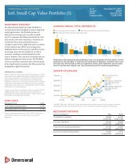
If the portfolio is never rebalanced, the allocation drifts from the initial 60/40 combination<br />
<strong>and</strong> becomes increasingly concentrated in stocks, as shown in the top panel<br />
of Exhibit 1. The equity allocation increases from 60% in 1926 to 90% by 1955, <strong>and</strong><br />
reaches 99.8% in 2008. The bottom panel of Exhibit 1 displays the weights in each<br />
asset class <strong>and</strong> shows that even within equities, the portfolio becomes overexposed<br />
to the highest-returning asset class. The Small Value portfolio initially had 8% of the<br />
portfolio allocation in 1927, but grew to 63% in 2008.<br />
To determine whether rebalancing increases returns, I compare the returns of the nonrebalanced<br />
portfolio to one that is simply rebalanced to target annually. Because 82<br />
years is a long time not to rebalance, even for an extremely long-lived <strong>and</strong> incredibly<br />
inattentive investor, I also consider cases where the portfolio is seldom rebalanced,<br />
at intervals of 5, 10, or 20 years. Because these rebalancing strategies do not require<br />
many trades, the effect of transactions cost would be minimal <strong>and</strong> are thus ignored in<br />
this analysis.<br />
The means <strong>and</strong> st<strong>and</strong>ard deviations for the rebalanced, seldom rebalanced, <strong>and</strong> never<br />
rebalanced portfolios are shown in Table 7. The non-rebalanced portfolio has greater<br />
return <strong>and</strong> greater volatility than the annually rebalanced <strong>and</strong> seldom rebalanced portfolios.<br />
This should come as no surprise, given the significant allocation to stocks in the<br />
non-rebalanced portfolio at the end of the period.<br />
Table 7<br />
Summary Statistics of Monthly <strong>Returns</strong><br />
July 1926-June 2008<br />
<strong>Rebalancing</strong> Frequency (years)<br />
1 5 10 20 Never<br />
Average Monthly Return 0.88% 0.85% 0.85% 0.89% 1.07%<br />
St<strong>and</strong>ard Deviation 4.04% 3.67% 3.61% 3.72% 4.59%<br />
Clearly, no meaningful comparison of returns can be made without controlling for<br />
risk. Fama <strong>and</strong> French (1993) show that average returns on stocks <strong>and</strong> bonds are well<br />
8. Kenneth R. French, “US Research <strong>Returns</strong> Data,” in http://mba.tuck.dartmouth.edu/pages/faculty/<br />
ken.french/data_library.html#Research.<br />
9. US bills, notes, <strong>and</strong> long-term bonds © Stocks, Bonds, Bills, <strong>and</strong> Inflation Yearbook, Ibbotson<br />
Associates, Chicago (annually updated work by Roger G. Ibbotson <strong>and</strong> Rex A. Sinquefield).
16<br />
<strong>Dimensional</strong> <strong>Fund</strong> <strong>Advisors</strong><br />
Exhibit 1<br />
Asset Allocation without <strong>Rebalancing</strong><br />
July 1926-June 2008<br />
Stocks <strong>and</strong> Bonds<br />
<br />
<br />
<br />
<br />
<br />
<br />
<br />
<br />
<br />
<br />
<br />
<br />
<br />
<br />
<br />
<br />
<br />
<br />
<br />
<br />
<br />
<br />
<br />
<br />
<br />
<br />
<br />
<br />
<br />
<br />
<br />
<br />
<br />
<br />
<br />
<br />
<br />
<br />
<br />
<br />
<br />
<br />
<br />
<br />
<br />
<br />
<br />
<br />
<br />
<br />
<br />
<br />
<br />
<br />
<br />
<br />
<br />
Asset Classes
<strong>Rebalancing</strong> <strong>and</strong> <strong>Returns</strong> 17<br />
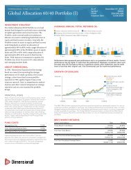
Exhibit 2<br />
Coefficients from Rolling Five-Factor Regressions<br />
June 1931-June 2008<br />
Non-Rebalanced<br />
<br />
<br />
<br />
<br />
<br />
<br />
<br />
<br />
<br />
<br />
<br />
<br />
<br />
<br />
<br />
<br />
<br />
<br />
<br />
<br />
<br />
<br />
<br />
Annually Rebalanced
18<br />
<strong>Dimensional</strong> <strong>Fund</strong> <strong>Advisors</strong><br />
explained by their exposures to five risk factors: the market return in excess of the onemonth<br />
Treasury bill rate (MKT), the return on small capitalization stocks in excess of the<br />
return on large capitalization stocks (SMB), the return on value stocks in excess of the<br />
return on growth stocks (HML), the return on long-term government bonds in excess of<br />
the one-month Treasury bill rate (TERM), <strong>and</strong> the return of long-term corporate bonds<br />
in excess of the return on long-term government bonds (DEF). Any return that cannot be<br />
explained by these five risk factors appears in the alpha term of a five-factor regression.<br />
The factor loadings on the five Fama/French risk factors are plotted for both the nonrebalanced<br />
<strong>and</strong> the annually rebalanced portfolios in Exhibit 2. Because the coefficients<br />
in the five-factor regression may not be constant over the entire 82-year sample,<br />
I estimate rolling five-factor regressions using the previous 60 months of data. For<br />
example, coefficients reported for December 1990 are estimated using monthly data<br />
from January 1986 to December 1990. The risk factor exposures display a tendency to<br />
trend in a particular direction in the non-rebalanced portfolio, as shown in the top panel<br />
of Exhibit 2. The TERM <strong>and</strong> DEF risk factors mainly explain bond returns, <strong>and</strong> thus it<br />
is no surprise that the exposures to these two factors tend to zero as the share of bonds<br />
in the non-rebalanced portfolio gets close to zero. The coefficient on the market factor<br />
increases from about 0.6 to 1, echoing the increasing overall share of stocks in the nonrebalanced<br />
portfolio. The loadings on SMB <strong>and</strong> HML also trend upward, reflecting the<br />
increased exposures to small <strong>and</strong> value stocks. In contrast, maintaining the targeted risk<br />
exposures, which should be the primary goal of rebalancing, is successfully achieved<br />
in the annually rebalanced portfolio. The factor loadings of the rebalanced portfolio,<br />
shown in the lower panel of Exhibit 2, are fairly stable over the entire sample.<br />
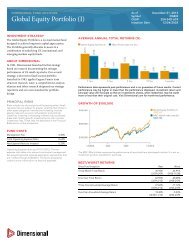
If rebalancing produces returns in excess of the risks captured by these five factors,<br />
the five-factor alphas of the rebalanced portfolio should be larger than the alpha of<br />
the portfolios that are seldom or never rebalanced. The differences in alpha, plotted<br />
in the upper panel of Exhibit 3, should be positive on average. Aside from some large<br />
positive differences in the 1930s, the alphas of the rebalanced portfolio do not appear<br />
to be reliably larger than the portfolios rebalanced seldom or never. In fact, looking at<br />
the t-statistics for the differences in the lower panel of Exhibit 3, these differences are<br />
significantly positive about the same number of times they are significantly negative.<br />
A few significant instances, both negative <strong>and</strong> positive, are exactly what one should<br />
expect from r<strong>and</strong>om noise given so many observations.<br />
The results from the analysis of 82 years of data highlight the danger when interpreting<br />
return differences over short samples. Over short samples, it is possible that rebalanced<br />
portfolios can have higher risk-adjusted returns than portfolios rebalanced infrequently or<br />
not at all. However, the historical data shows that the reverse also occurs. Over the entire<br />
82-year sample, it is clear that the rebalanced portfolio had no significant advantage over<br />
the portfolios rebalanced less frequently. It would be premature to declare the existence<br />
of positive rebalancing return benefits using 10 to 20 years of data because the period is<br />
too short <strong>and</strong> the data is too volatile to distinguish higher expected returns from luck.
<strong>Rebalancing</strong> <strong>and</strong> <strong>Returns</strong> 19<br />
Exhibit 3<br />
Difference in Alphas from Rolling Five-Factor Regressions<br />
June 1931-June 2008<br />
Annually Rebalanced Alpha – Infrequent or Never Rebalanced Alpha<br />
<br />
<br />
<br />
<br />
<br />
<br />
<br />
<br />
<br />
<br />
<br />
<br />
<br />
<br />
<br />
<br />
<br />
<br />
<br />
<br />
<br />
<br />
T-Statistic
20<br />
<strong>Dimensional</strong> <strong>Fund</strong> <strong>Advisors</strong><br />
Conclusions<br />
While it is true that the details of a rebalancing strategy will affect portfolio returns,<br />
trying to predict which strategy will have the highest returns going forward will likely<br />
lead one down a path of unproductive data mining. It is fairly easy to search over a<br />
number of strategies to find the one that works the best in a given sample <strong>and</strong> for a<br />
particular portfolio. However, finding one that will continue to provide better returns<br />
out of sample is a much more difficult if not impossible task.<br />
Aside from avoiding excessive trading, there are no optimal rebalancing rules that<br />
will yield the highest returns on all portfolios <strong>and</strong> in every period. The good news for<br />
investors is that without an optimal way to rebalance, the burden of producing returns<br />
through optimal rebalancing is lifted. Return generation is again the responsibility of<br />
the market, which sets prices to compensate investors for the risks they bear. The primary<br />
motivation for rebalancing should not be the pursuit of higher returns, as returns<br />
are determined through the asset allocation, not through rebalancing.<br />
The bad news, of course, is that there is no easy one-size-fits-all rebalancing solution.<br />
<strong>Rebalancing</strong> decisions should be driven by the need to maintain an allocation with a<br />
risk <strong>and</strong> return profile appropriate for each investor. The optimal rebalancing strategy<br />
will differ for each investor, depending on their unique sensitivities to deviations from<br />
the target allocation, transaction frequency, <strong>and</strong> tax costs.<br />
References<br />
Clark, Truman A. 1999. “Efficient portfolio rebalancing.” <strong>Dimensional</strong> <strong>Fund</strong> <strong>Advisors</strong><br />
working paper (January).<br />
Clark, Truman A. 2003. “<strong>Rebalancing</strong>: When, how, <strong>and</strong> why.” <strong>Dimensional</strong> <strong>Fund</strong> <strong>Advisors</strong><br />
working paper (April).<br />
Daryanani, Gobind. 2008. “Opportunistic rebalancing: A new paradigm for wealth<br />
managers.” Journal of Financial Planning 21 (1):48-61.<br />
Fama, Eugene F., <strong>and</strong> Kenneth R. French. 1993. “Common risk factors in the returns<br />
on stocks <strong>and</strong> bonds.” Journal of Financial Economics 33:3-56.<br />
Lel<strong>and</strong>, Hayne E. 1996. “Optimal asset rebalancing in the presence of transactions costs.”<br />
University of California, Berkeley Haas School of Business working paper (March).<br />
Plaxco, Lisa M., <strong>and</strong> Robert D. Arnott. 2002. “<strong>Rebalancing</strong> a global policy benchmark.”<br />
Journal of Portfolio Management 28 (2):9-22.