RocFrac User's Guide

RocFrac User’s Guide 

by M. Scot Breitenfeld 1 

12th December 2005 

1 This file is currently maintained by SCOT BREITENFELD, brtnfld@uiuc.edu. Please send comments or 

error corrections to that address.

Contents 

1 RocFrac Command Statements 3 

1.1 Compiling . . . . . . . . . . . . . . . . . . . . . . . . . . . . . . . . . . . . . . . . . . . . 3 

1.2 Sequence Needed to Run a Problem . . . . . . . . . . . . . . . . . . . . . . . . . . . . . 3 

1.2.1 Create Finite Element Mesh/Steps needed with Patran . . . . . . . . . . . . . 3 

1.2.1.1 Geometry Creation . . . . . . . . . . . . . . . . . . . . . . . . . . . . . . 3 

1.2.1.2 Mesh Creation . . . . . . . . . . . . . . . . . . . . . . . . . . . . . . . . 4 

1.2.1.3 Monitoring nodes and elements . . . . . . . . . . . . . . . . . . . . . . 4 

1.2.1.4 Boundary Condition Flags . . . . . . . . . . . . . . . . . . . . . . . . . 4 

1.2.2 Controlling what surface is in contact with the the fluids domain . . . . . . . 6 

1.2.3 Setting element flags . . . . . . . . . . . . . . . . . . . . . . . . . . . . . . . . . 7 

1.2.4 Run rfracprep . . . . . . . . . . . . . . . . . . . . . . . . . . . . . . . . . . . . . . 8 

1.2.5 Run RocFrac . . . . . . . . . . . . . . . . . . . . . . . . . . . . . . . . . . . . . . 8 

1.2.6 Run the Post-processor . . . . . . . . . . . . . . . . . . . . . . . . . . . . . . . . 9 

1.3 File Management . . . . . . . . . . . . . . . . . . . . . . . . . . . . . . . . . . . . . . . . 9 

2 Executive Control Section 10 

2.1 Executive System Parameters . . . . . . . . . . . . . . . . . . . . . . . . . . . . . . . . 10 

2.1.1 *PREFIX: Define the prefix extension for IO files. . . . . . . . . . . . . . . . . . 10 

2.1.2 *NRUN: Define the timing parameters** (Obsolete) . . . . . . . . . . . . . . . . 10 

2.1.3 *DYNAMIC: . . . . . . . . . . . . . . . . . . . . . . . . . . . . . . . . . . . . . . . 10 

2.1.4 *ALE: Enable ALE . . . . . . . . . . . . . . . . . . . . . . . . . . . . . . . . . . . 11 

2.1.5 *IOPARAM: Output options . . . . . . . . . . . . . . . . . . . . . . . . . . . . . . 11 

2.1.6 *IOFORMAT: Format of input files . . . . . . . . . . . . . . . . . . . . . . . . . . 11 

2.1.7 *POVIO: Output POV-RAY format . . . . . . . . . . . . . . . . . . . . . . . . . . 11 

2.1.8 *HYPERELASTIC: hyperelastic material model . . . . . . . . . . . . . . . . . . . 11 

2.1.9 *MICROMECHANICAL: micromechanical material model . . . . . . . . . . . . 12 

2.1.10*ELASTIC: elastic material model . . . . . . . . . . . . . . . . . . . . . . . . . . 12 

2.1.11*MATVOL: Volumetric element material properties** (Obsolete) . . . . . . . . . 13 

2.1.12*MATCOH: Cohesive element properties . . . . . . . . . . . . . . . . . . . . . . 13 

2.1.13*PLOAD: Static Pressure Load . . . . . . . . . . . . . . . . . . . . . . . . . . . . 13 

2.1.14*PLOAD1: Dynamic Pressure Load . . . . . . . . . . . . . . . . . . . . . . . . . 14 

2.1.15*DUMMYTRACT: Assigns a traction when Rocfrac Stand alone is used . . . . 14 

2.1.16*DUMMYFLUX: Assigns a heat flux when Rocfrac Stand alone is used . . . . 14 

2.1.17*DUMMYBURN: Assigns a burn rate when Rocfrac Stand alone is used . . . . 14 

2.1.18*END: Denotes end of control deck input . . . . . . . . . . . . . . . . . . . . . . 14 

2.1.19*BOUNDARY: Displacement Boundary Conditions . . . . . . . . . . . . . . . . 15 

2.1.20*BOUNDARYMM: Mesh Motion Boundary Conditions . . . . . . . . . . . . . . 15 

2.1.21*BOUNDARYHT: Thermal Boundary Conditions . . . . . . . . . . . . . . . . . . 15 

2.1.22*INITIAL CONDITION: assigns the initial conditions . . . . . . . . . . . . . . . 15 

2.1.23*ELEMENT: Element Type . . . . . . . . . . . . . . . . . . . . . . . . . . . . . . 16 

2.1.24*DAMPING . . . . . . . . . . . . . . . . . . . . . . . . . . . . . . . . . . . . . . . 16 

2.1.25*HEAT TRANSFER . . . . . . . . . . . . . . . . . . . . . . . . . . . . . . . . . . . 16 

1

CONTENTS 

2.1.26*PROBE . . . . . . . . . . . . . . . . . . . . . . . . . . . . . . . . . . . . . . . . . 17 

3 Three-dimensional solid element library 18 

3.1 Volumetric Stress/Displacement Elements: . . . . . . . . . . . . . . . . . . . . . . . . 18 

3.2 Cohesive Stress/Displacement Elements: . . . . . . . . . . . . . . . . . . . . . . . . . 18 

4 RocFrac Input File (old format) 20 

4.1 Data Format . . . . . . . . . . . . . . . . . . . . . . . . . . . . . . . . . . . . . . . . . . 20 

5 Example Problems 24 

5.1 Layered Two Material Cantilever Beam . . . . . . . . . . . . . . . . . . . . . . . . . . . 24 

2

Chapter 1 

RocFrac Command Statements 

The purpose of RocFrac is to simulate complex dynamic fracture problems using an explicit 

Cohesive Volumetric Finite Element (CVFE) scheme. RocFrac can handle large deformations, 

moving interfaces, and non-linear material response. 

1.1 Compiling 

The source files and makefile for the analysis code resides in the directory Rocfrac/Source in 

the RocStar tree. The source files and makefile for the preprocessor rfracprep reside in the 

directory Rocfrac/utilities/RocfracPrep. The preprocessor rfracprep is automatically build within 

the Rocstar suite. 

1.2 Sequence Needed to Run a Problem 

This section describes the sequence of execution needed to run RocFrac. In general there are 4 

steps involved: create the finite element mesh, partition the mesh and add cohesive elements (if 

required), solution and post-processing. 

1.2.1 Create Finite Element Mesh/Steps needed with Patran 

The first step is to create the finite element mesh. As of this writing there is only one practical way 

to create the volumetric finite element mesh and that is to use the commercial package Patran. 

Please refer to the Patran documentation on how to use Patran for creating meshes. If Patran is 

used at NCSA then the user is limit to creating meshes no greater then roughly 1 million elements 

before needing to submit the Patran job as batch. Once the mesh and boundary conditions have 

been created the file needs to be exported to a Patran Neutral File. The file should have the same 

prefix as that found in the control deck file under the option *PREFIX. The ending suffix of the 

neutral file must end in ’.pat’ or ’.out’. Thus, the name convention is PREFIX.out or PREFIX.pat. 

This file should be placed in the Modin directory in located in the Rocfrac directory of the Rocstar 

suite. 

1.2.1.1 Geometry Creation 

There are no special considerations to be address. 

would proceed to do for a finite element calculation. 

The geometry can be created just as one 

3

1.2. SEQUENCE NEEDED TO RUN A PROBLEM 

1.2.1.2 Mesh Creation 

There are no special considerations that need to be taken when creating a finite element mesh, 

just engineering judgment. Note, however, that the only elements currently supported by Rocfrac 

are: 4 and 10 node tetrahedral elements for an Arbitrary Euler Lagrange (*ALE) calculation and 

8 node hexahedral, 4 and 10 node tetrahedral for non-ALE calculations. Currently the use of 

mixed meshes in modeling the geometry is not permitted. 

For very large meshes it is useful to split the mesh into sections if possible. An example is a 4 

segment rocket with no case. Each segment can be meshed independently and written to a Patran 

neutral file. The mesh files are then placed in Rocfrac/Modin with the the file name PREFIX.#.out 

where # is the number of the segment starting from 1. Note: each mesh’s numbering of elements 

and nodes must start from 1. 

1.2.1.3 Monitoring nodes and elements 

To specify nodes or elements to monitor during the simulation use the Create -> Temperature 

Boundary Conditions dialog. Actual values give as boundary condition is ignored, BC is only 

used to mark monitored nodes and elements. 

1.2.1.4 Boundary Condition Flags 

The boundary conditions set in Patran are not the actual boundary conditions for the model, but 

instead represent flags that denote the actual boundary conditions. 

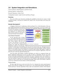
Setting the Displacement Boundary Condition Flags 

The way to set the boundary condition for the displacement boundary conditions is to assign the 

U x fixed displacement the appropriate flag as that found in the control deck option *BOUNDARY 

(See Section 2.1.19). For example, if the top of a specimen is to be fixed in all three directions 

then the U x fixed displacement should be given a value of 1.0 in Patran, which will correspond 

to the boundary condition specified in card 1 under the *BOUNDARY option. 

4


Patran dialog box to set displacement boundary conditions 

Setting the Mesh Motion Boundary Condition Flags 

The way to set the boundary condition for the mesh motion boundary conditions is to use the 

’create displacement dialog box’ and assign the U z displacement the appropriate flag as that 

found in the control deck option *BOUNDARYMM (See Section 2.1.20). For example, if the top of 

a specimen is to have fixed velocities in all three directions then the U z displacement should be 

given a value of 1.0 in Patran, which will correspond to the boundary condition specified as card 

1 under the *BOUNDARYMM option. 

Setting the Mesh Motion Boundary Condition Flags 

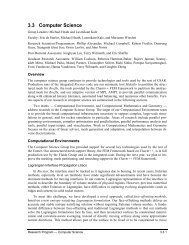
Setting the Thermal Boundary Conditions 

The way to set the boundary condition for the thermal boundary conditions is to use the ’create 

displacement dialog box’ and assign the U y displacement the appropriate flag as that found in the 

control deck option *BOUNDARYHT (See Section 2.1.20). For example, if the top of a specimen 

is to have fixed temperature then the U y displacement should be given a value of 1.0 in Patran, 

which will correspond to the boundary condition specified as card 1 under the *BOUNDARYHT 

option. 

5


Setting the Thermal Boundary Condition Flags 

1.2.2 Controlling what surface is in contact with the the fluids domain 

To specify which surfaces are in contact with the fluids domain we use Patran’s ’apply pressure’ 

dialog box. On the surfaces that are in contact with the fluids domain use a pressure value equal 

to 1 for non-inert surfaces or 2 for inert surfaces . To specify a surface that is not in contact with 

the fluids domain we use a pressure value of 0. To specify a surface that is between two solids 

domain use the value of 4 on one surface and 5 on the opposite surface. 

6


1.2.3 Setting element flags 

To specify the element flags using Patran for the volumetric flags we use the ’properties’ option. 

Assign an element property to each volume where you want a different property. Note that you 

should not use the material property window. 

7


1.2.4 Run rfracprep 

The Patran Neutral Files should be placed in the Rocfrac/ModIn directory. The program rfracprep 

creates the cohesive elements (if needed) and partitions the mesh using the program METIS. It 

currently only supports the inclusion of cohesive elements everywhere in the domain and only 

between tetrahedral elements. To run type: rfracprep in the same directory as the Rocfrac- 

Control.txt file. Execution is self-explanatory and two command line options are available; -np 

# tells rfracprep how many processors to partition the mesh and -un # (where # is the units 

conversion factor) is used to convert the units of the geometry. rfracprep will then create each 

processor’s input file in the directory Rocfrac/Rocin/ and each volumetric mesh file will be called 

.####.hdf where #### corresponds to the processor’s id. It will also create the 2D 

(SurfMesh.####.hdf) interface meshes needed to be registered with RocCom via RocFrac. The 

final file that needs to be created by your favorite editor (emacs/vi..) is the input control deck file 

RocfracControl.txt, see Section 2.1. 

1.2.5 Run RocFrac 

The program RocFrac is part of the RocStar code, so it must be run within the RocStar framework. 

In order to run it in Stand-Alone mode (i.e. no other RocStar modules are needed), the 

option ’SolidAlone Rocflo Rocfrac Rocburn’ can be specified, thus allowing for a Rocfrac alone 

analysis problem. In order to run a stand alone problem, the pressure and burning rate needs to 

be applied within RocFrac since these quantities are not supplied from the fluid or burning modules. 

During the analysis the results output files are written to the Rocfrac/Rocout/ directory. 

These HDF files consist of: surface meshes results (isolid_*.hdf), volume meshes (solid_*hdf), and 

restart quantities (solid_bnd*.hdf). Note, as of this writing, for the restart, it must be restarted 

on the same number of processors for each run. 

8

1.3. FILE MANAGEMENT 

1.2.6 Run the Post-processor 

The isolid_*.hdf and solid_*.hdf files are used in Rocketeer to view the results. The solid_bnd*.hdf 

files are not to be used in Rocketeer, there’re only used for restarting. 

1.3 File Management 

• RocfracControl.txt - control deck input file. See Section 2.1 for a description of the control 

deck parameters. This file should be placed in the Rocfrac/ directory in the GenX tree. 

• Modin/.pat - Patran Neutral File. 

• Rocin/.####.inp - each processor’s input file. 

• .res - output file, summarizes the input data from the control deck. 

• Rocout/*.hdf - Rocketeer input and restart. 

9

Chapter 2 

Executive Control Section 

This section describes the keywords and specifications for the input control deck file. The control 

deck file contains keyword statements that correspond to the analysis. The format definitions 

are as follows: A - character, F - real, I - integer. Keyword cards must begin with a * in column 1. 

These keywords and keyword specifics are based on Abaqus’s. For a more in-depth description 

the reader should consult the abaqus keyword manual. 

2.1 Executive System Parameters 

2.1.1 *PREFIX: Define the prefix extension for IO files. 

This option allows the user to specify what the prefix extensions are for the input files and 

the output files. The prefix should be no more then 20 characters in length. NOTE: ALWAYS 

NEEDED 

Option Format Entry 

First card: 

1 A prefix name 

2.1.2 *NRUN: Define the timing parameters** (Obsolete) 

This option is used to specify the parameters needed to obtain a stable solution. NOTE: ALWAYS 

NEEDED 


First card: 

2 I divide the courant condition time step by 

Note: typical values are 1.0-4.0 depending on whether ALE was specified. 

2.1.3 *DYNAMIC: 

This option is used to specify the parameters needed to obtain a stable solution. NOTE: ALWAYS 

NEEDED 

‡Optional Parameters: 

SCALE FACTOR 

10

2.1. EXECUTIVE SYSTEM PARAMETERS 

ALE 

Factor to multiply the Courant limit, typical values are .8 - .9 without ALE and .5-.8 with 

First card: No cards 

2.1.4 *ALE: Enable ALE 

This option is used to run an ALE simulation (the default is off if not specified). 


First card: 

2 I mesh motion stability parameter 

Note: typical values are between .1-.3 

2.1.5 *IOPARAM: Output options 

This option is used to specify the output interval to write results to a file that will later be postprocessed. 

If the option is not given then the default is to never output the results to a file. 


First card: 

1 I time step interval for output 

2.1.6 *IOFORMAT: Format of input files 

This option is used to specify the format of the input file. If the value equals 1 then the input 

files are ASCII and if the value equals 0 then the input files are binary. 

2.1.7 *POVIO: Output POV-RAY format 

This option is used to specify that the outer boundary of the mesh should be written to a file 

for further analysis with the pov-ray ray tracing program. The output files need first to be run 

through the post pov-ray program. If the option is not given then the default is not to write any 

pov-ray files. 


First card: 

1 F value to magnify the displacement 

2 I time step to start the output 

3 I interval for output 

2.1.8 *HYPERELASTIC: hyperelastic material model 

Specifies a hyperelastic volumetric elements material model. 


NEOHOOKINC 

Specifies the Incompressible neo-Hookean model 

ARRUDA-BOYCE 

Specifies the ARRUDA-BOYCE material model, good for filled rubbers 

11



First card: 

1 I total number of materials 

Following cards: 

1 F Young’s Modulus 

2 F Poisson’s Ratio 

3 F Density 

4 F Thermal Expansion Coefficient 

2.1.9 *MICROMECHANICAL: micromechanical material model 

Specifies a micromechanical volumetric elements material model. 


MODEL=HUANG 

Specifies the micromechanical model developed by Prof. Huang 

MODEL=MATOUS ** (under development) 

Specifies the micromechanical model developed by Karl Matous 


First card: 

1 F Matrix Young’s Modulus 

2 F Matrix Poisson’s Ratio 

2 F Matrix volume fraction 

3 F Composite Density 

1 I total number of particles 


1 F Particle Young’s Modulus 

2 F Particle Poisson’s Ratio 

3 F Particle volume fraction 

4 F Particle size 

2.1.10 *ELASTIC: elastic material model 

Specifies a elastic volumetric elements material model. 


NLGEOM 

Specifies finite rotations 


First card: 





3 F Density 


12


2.1.11 *MATVOL: Volumetric element material properties** (Obsolete) 

Specifies the volumetric elements material properties. NOTE: ALWAYS NEEDED 


First card: 





3 F Density 


5 F Material type analysis 

For card 5, the current options are: 

0 - non-linear arruda-boyce 

1 - large deformation, linear material 

2 - small deformation, linear material 

-1 - Neo-Hookean Incompressible 

11 - Neo-Hookean Incompressible, Node based formulation 

13 - large deformation, linear material, Node based formulation 

2.1.12 *MATCOH: Cohesive element properties 

Specifies the cohesive elements properties. 


First card: 

1 I total number of properties 


1 F Critical normal opening displacement 

2 F Critical tangential opening displacement 

3 F Critical tensial stress 

4 F Critical shearing stress 

5 F Initial Stress threshold 

2.1.13 *PLOAD: Static Pressure Load 

Defines the pressure value for a static pressure load on a triangular surface elements. Need a 

.press file to give a list of the surface triangles where the pressure is applied. 


First card: 

1 I Pressure 

13


2.1.14 *PLOAD1: Dynamic Pressure Load 

Specifies that the load changes with each time step, the pressure values are read in from an 

input file for each time step. The file name should be no longer then 20 characters. 


First card: 

1 A file name containing the nodal pressure values 

2.1.15 *DUMMYTRACT: Assigns a traction when Rocfrac Stand alone is 

used 

The magnitude of the traction force applied, the region that the traction gets applied to is specified 

in the RocFracUpdateInbuff subroutine. 


INTERFACE = SF 

Apply pressure on surfaces marked Fluid/Solid interface 

INTERFACE = S 

Apply pressure on surfaces marked Solid interface 

INTERFACE = ALL 

Apply pressure on all surfaces 



First card: 

1 F Traction magnitude value 

2.1.16 *DUMMYFLUX: Assigns a heat flux when Rocfrac Stand alone is 

used 

The magnitude of the heat flux applied, the region that the traction gets applied to is specified in 

the RocFracUpdateInbuff subroutine. 


First card: 


2.1.17 *DUMMYBURN: Assigns a burn rate when Rocfrac Stand alone is 

used 

The magnitude of the burn rate applied, the region that the traction gets applied to is specified 

in the RocFracUpdateInbuff subroutine. 


First card: 


2.1.18 *END: Denotes end of control deck input 

Place at the end of the control deck input key variables. No options. NOTE: ALWAYS NEEDED 

14


2.1.19 *BOUNDARY: Displacement Boundary Conditions 

Specifies the meaning of the boundary condition flags set in the meshing program. A zero indicates 

that the boundary condition is an imposed velocity and a one is for an imposed force. Only 

the last three parameters should be changed to the specific value for each card. Note *BOUND- 

ARY is not used by the analysis code but only by the preprocessor, hence *BOUNDARY should 

always be placed before the *END option. 


First to number of boundary flags: 

10 0 0 3E value x, value y, value z 


2.1.20 *BOUNDARYMM: Mesh Motion Boundary Conditions 

Specifies the meaning of the mesh motion boundary condition flags set in the meshing program. 

A zero indicates that the boundary condition is an imposed velocity and a one is for an imposed 

force. 





2.1.21 *BOUNDARYHT: Thermal Boundary Conditions 

Specifies the meaning of the thermal boundary condition flags set in the meshing program. A zero 

indicates that the boundary condition is an imposed temperature and a one is for an imposed 

heat flux. 





2.1.22 *INITIAL CONDITION: assigns the initial conditions 

The magnitude of the initial conditions of the simulation. 


TYPE = TEMPERATURE 

Initial reference temperature. 



First card: 

1 F Initial Temperature 

15


2.1.23 *ELEMENT: Element Type 

Specifies the volumetric element type. 


V3D4 

4 node tetrahedral 

V3D4NCC 

4 node tetrahedral, node based element, lumped using circumcenter 

V3D4N 

4 node tetrahedral, node based element, lumped using centroid 

V3D10R 

10 node tetrahedral, reduced integration 

V3D10 

10 node tetrahedral 

V3D8ME 

8 node hexahedral mixed enhanced 

2.1.24 *DAMPING 

Specifies artifical damping. 

2.1.25 *HEAT TRANSFER 

Specifies material properties for heat transfer analysis 


First card: 



1 F Thermal conductivity, κ 

2 F Specific heat at constant pressure, C p 

16


2.1.26 *PROBE 

Monitors variables at a point in space given in Cartesian coordinates. Note: the node closest 

to the specified coordinates will be flag to be monitored. Probe data is written to the Rocout 

directory. 


1 I total number of probes 


1 3E Coor. x, Coor. y, Coor. z 

17

Chapter 3 

Three-dimensional solid element 

library 

This section defines the three-dimensional solid (continuum) elements available in RocFrac. 

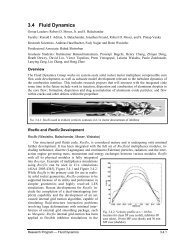
3.1 Volumetric Stress/Displacement Elements: 

• V3D4 4-node linear tetrahedron 

• V3D10 10-node quadratic tetrahedron 

• V3D8 8-node hexahedral 

Warning: Element type C3D4 is a constant stress tetrahedron. This element only provides 

accurate results in general cases with very fine meshing. 

Active degrees of freedom: 

1, 2, 3 (u x ,u y , u z ) 

4 

2 

4 

3 

3 

8 

4 

7 

9 

10 

3 

z 

y 

1 

x 

1 

2 

4−node element 

1 

6 

5 

2 

10−node element 

Figure 3.1: Node ordering and face numbering for tetrahedral elements 

3.2 Cohesive Stress/Displacement Elements: 

• C3D6 6-node linear triangular prism with 3-point gauss integration. 

• C3D12 12-node quadratic triangular prism (NOT YET IMPLEMENTED) 

18

3.2. COHESIVE STRESS/DISPLACEMENT ELEMENTS: 

Active degrees of freedom: 

1, 2, 3 (∆u x ,∆u y , ∆u z ) 

3 

5 

∆ 

1 

∆ 

1 

2 

6−node cohesive element 

3 

4 

∆ 

2 

6 

9 

3 

∆ 

5 

10 

8 

∆ 

1 7 2 

4 

∆ 

5 

4 

6 

11 

12 

6 

12−node cohesive element 

Figure 3.2: Node ordering for cohesive elements 

19

Chapter 4 

RocFrac Input File (old format) 

The Input Files ( i.e. the /.N#.inp files, where N# is the processors id) are used 

to communicate the analysis model into Rocfrac standalone version. Each processor has its own 

input file. File format was replace in Gen3 with HDF formatted files. 

4.1 Data Format 

The input files format is as follows: 

Packet 01: Version Number 

Data Card 1 

VERS 

VERS = Version Number of Analysis Code 

Packet 02: Node Data 

Data Card 1 

N1, Aux, Aux, Aux, Aux 

N1 = Number of Nodes 

Aux = Auxilllary flags (not applicable) 

Data Card 2 (Repeated N1 times) 

ID X Y NDFLAG1 

X = X Cartesian Coordinate of Node 

Y = Y Cartesian Coordinate of Node 

Z = Z Cartesian Coordinate of Node 

NFLAG1 = Generic Flag of Node (not applicable) 

Packet 03: Structural Boundary Conditions 

Data Card 1 

20

4.1. DATA FORMAT 

NumBC, AuxFlag 

NumBC = Number of Boundary Condition Flags 

AuxFlag = Auxillary Flag (not applicable) 

Data Card 2 (Repeated NumBC times) 

NodeID BCFLAG1 BCFLAG2 

NodeID = Node Identification 

BCFLAG1 = Boundary Condition Flag 1 

BCFLAG2 = Boundary Condition Flag 2 (not applicable) 

Packet 04: Mesh Motion Boundary Conditions 

Data Card 1 

NumBC, AuxFlag 

NumBC = Number of Boundary Condition Flags 

AuxFlag = Auxillary Flag (not applicable) 

Data Card 2 

NodeID BCFLAG1 BCFLAG2 

NodeID = Node Identification 

BCFLAG1 = Boundary Condition Flag 1 

BCFLAG2 = Boundary Condition Flag 2 (not applicable) 

Packet 05: Element Data 

Data Card 1 

21


NumElemProp 

ElemPropId 

NumElemType 

ElemType, NumEl, NumElBndry 

MatId, ElemConn, AUX 

NumElemProp = Total Number of Element Properties 

ElemPropId = Element Property Id 

NumElemType = Number of Element Types 

ElemType: 

1D - Bar0002, Bar0003, Bar0004 

2D - tri0003, tri0004, tri0006,tri0007, tri0009, tri0013 

2D - quad004, quad005, quad008,quad009, quad014, 

quad015 

3D - tet0004, tet0010, tet0016 

3D - wedge06, wedge07, wedge15, wedge16, 

wedge20,wedge21, wedge24, wedge52 

3D - hex0008, hex0009=26, 

hex0020,hex0021,hex0026,hex0027,hex0032,hex0064 

NumEl = Total Number of ’ElemType’ Elements 

NumElBndry = Total Number of Partition Border ’ElemType’ 

Elements 

MatId = Element Material Id 

ElemConn = Element corner nodes followed by additional 

nodes 

AUX = Auxillary Input (not applicable) 

Data Card 2 

IMAT, LND, AUX, AUX 

IMAT = Material ID 

LND = Element corner nodes followed by additional nodes 

NumElTot = Number of Elements Total 



Packet 06: Parallel Communication 

Data Card 1 

NumNeigh 

NumNeigh = Number of Neighboring Processors 

Data Card 2 (Repeated NumNeigh times) 

NeighID,NumNodeShare 

NeighID = Neighbor’s ID 

NumNodeShare = Number of Shared Nodes with NeighID 

22


Data Card 3 (Repeated NumNodeShare times) 

NodeShareID 

NodeShareID = ID of shared node 

Packet Type 99: 

Data Card 1 

99 

Signals End of Input File 

23

Chapter 5 

Example Problems 

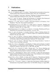
5.1 Layered Two Material Cantilever Beam 

This example is of a cantilever beam composed of two materials. The top half of the beam is 

composed of a rubber and the bottom half steel, shown in Figure 5.1. The rubber has a Young’s 

Modulus of 0.991 GPa, Poisson’s ratio of .46, Density of 956.0 kg/m 3 and is to be modeled using 

the NeoHookean Incompressible material model. The steel has a Young’s Modulus of 210 GPa, 

Poisson’s ratio of .27, density = 7870.9 kg/m 3 and is to be modeled using small displacements 

and linear material response. The traction load is 100.0 and the points are all fixed at the wall. 

¢¡¢ 

¢¡¢ 

¢¡¢ 

¢¡¢ 

¢¡¢ 

¢¡¢ 

¢¡¢ 

¢¡¢ 

¢¡¢ 

¢¡¢ 

¢¡¢ 

¢¡¢ 

¢¡¢ 

¢¡¢ 

¢¡¢ 

¢¡¢ 

Figure 5.1: Geometry and loading condition 

The input files for a four processor run can be found in cvs at /CSAR/brtnfld/GenXData/Beam2Mat. 

24

RocFrac User's Guide

You also want an ePaper? Increase the reach of your titles

Delete template?

Save as template?