Computational Modeling of Synthetic Jets - COMSOL.com
Computational Modeling of Synthetic Jets - COMSOL.com
Computational Modeling of Synthetic Jets - COMSOL.com

You also want an ePaper? Increase the reach of your titles
YUMPU automatically turns print PDFs into web optimized ePapers that Google loves.
Excerpt from the Proceedings <strong>of</strong> the <strong>COMSOL</strong> Conference 2010 Boston<br />
<strong>Computational</strong> <strong>Modeling</strong> <strong>of</strong> <strong>Synthetic</strong> <strong>Jets</strong><br />
David C. Durán *,1 , Omar D. López 2<br />
1 Mechanical Engineering Department, Universidad de los Andes, Bogotá - Colombia<br />
*Corresponding author: Carrera 1ra No. 18A-12, da-duran@uniandes.edu.co<br />
Abstract: A synthetic Jet actuator is a<br />
device which moves a fluid in and outside a cavity,<br />
through a small aperture, by the continuous<br />
oscillation <strong>of</strong> a diaphragm. This diaphragm is<br />
usually a piezoelectric disk which is excited by a<br />
sinusoidal voltage. The first approach to the<br />
problem was to validate the behavior <strong>of</strong> the<br />
piezoelectric disk through a tridimensional model,<br />
showing satisfactory results. After this validation<br />
an axisymmetric model <strong>of</strong> the <strong>com</strong>plete (fluid +<br />
piezoelectric) synthetic jet actuator was<br />
implemented. This model was used to analyze the<br />
influence <strong>of</strong> the relevant dimensionless numbers in<br />
the synthetic jet formation when the disk was<br />
excited at low frequencies. Numerical results <strong>of</strong><br />
this model show a strong dependence <strong>of</strong> the<br />
synthetic jet formation on the size <strong>of</strong> the aperture.<br />
Another relevant observation is that, for the case <strong>of</strong><br />
synthetic jet formation, there is an interaction<br />
between the entering momentum and the<br />
diaphragm, which has not been observed in other<br />
synthetic jet models based only on Navier-Stokes<br />
solver. All these observations are <strong>of</strong> great help in<br />
synthetic jet device research and development, and<br />
encourage further multiphysics simulations and<br />
analysis <strong>of</strong> these actuators to be made.<br />
Keywords: <strong>Synthetic</strong> Jet, Synjet, Structure-Fluid<br />
Interaction, Piezoelectric, Vortices<br />
1. Introduction<br />
A <strong>Synthetic</strong> Jet is defined as the time-averaged<br />
formation <strong>of</strong> escaping vortex rings from a cavity<br />
through which a fluid is suctioned and expelled,<br />
having a zero mass net flux but adding momentum<br />
to the surroundings. The device which generates<br />
<strong>Synthetic</strong> <strong>Jets</strong> is called a <strong>Synthetic</strong> Jet Actuator<br />
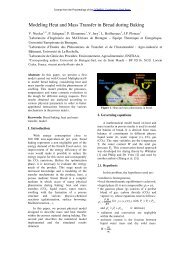
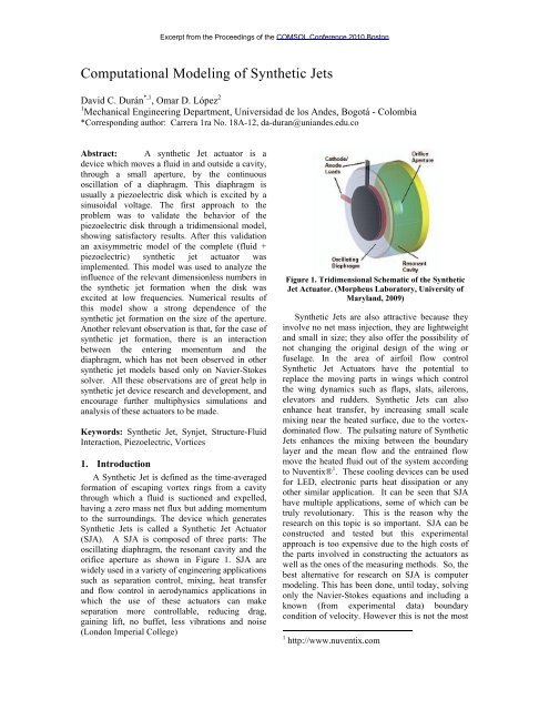
(SJA). A SJA is <strong>com</strong>posed <strong>of</strong> three parts: The<br />
oscillating diaphragm, the resonant cavity and the<br />
orifice aperture as shown in Figure 1. SJA are<br />
widely used in a variety <strong>of</strong> engineering applications<br />
such as separation control, mixing, heat transfer<br />
and flow control in aerodynamics applications in<br />
which the use <strong>of</strong> these actuators can make<br />
separation more controllable, reducing drag,<br />
gaining lift, no buffet, less vibrations and noise<br />
(London Imperial College)<br />
Figure 1. Tridimensional Schematic <strong>of</strong> the <strong>Synthetic</strong><br />
Jet Actuator. (Morpheus Laboratory, University <strong>of</strong><br />
Maryland, 2009)<br />
<strong>Synthetic</strong> <strong>Jets</strong> are also attractive because they<br />
involve no net mass injection, they are lightweight<br />
and small in size; they also <strong>of</strong>fer the possibility <strong>of</strong><br />
not changing the original design <strong>of</strong> the wing or<br />
fuselage. In the area <strong>of</strong> airfoil flow control<br />
<strong>Synthetic</strong> Jet Actuators have the potential to<br />
replace the moving parts in wings which control<br />
the wing dynamics such as flaps, slats, ailerons,<br />
elevators and rudders. <strong>Synthetic</strong> <strong>Jets</strong> can also<br />
enhance heat transfer, by increasing small scale<br />
mixing near the heated surface, due to the vortexdominated<br />
flow. The pulsating nature <strong>of</strong> <strong>Synthetic</strong><br />
<strong>Jets</strong> enhances the mixing between the boundary<br />
layer and the mean flow and the entrained flow<br />
move the heated fluid out <strong>of</strong> the system according<br />
to Nuventix® 1 . These cooling devices can be used<br />
for LED, electronic parts heat dissipation or any<br />
other similar application. It can be seen that SJA<br />
have multiple applications, some <strong>of</strong> which can be<br />
truly revolutionary. This is the reason why the<br />
research on this topic is so important. SJA can be<br />
constructed and tested but this experimental<br />
approach is too expensive due to the high costs <strong>of</strong><br />
the parts involved in constructing the actuators as<br />
well as the ones <strong>of</strong> the measuring methods. So, the<br />
best alternative for research on SJA is <strong>com</strong>puter<br />
modeling. This has been done, until today, solving<br />
only the Navier-Stokes equations and including a<br />
known (from experimental data) boundary<br />
condition <strong>of</strong> velocity. However this is not the most<br />
1 http://www.nuventix.<strong>com</strong>
ealistic approach to the problem since it ignores<br />
the multiphysics nature <strong>of</strong> the actuator. Willing to<br />
take into account the multiphysics nature <strong>of</strong> the<br />
problem and trying to make simulations more<br />
realistic, we modeled a SJA in <strong>COMSOL</strong><br />
Multiphysics and studied the influence <strong>of</strong> different<br />
parameters in the SJ formation.<br />
2. Use <strong>of</strong> <strong>COMSOL</strong> Multiphysics<br />
2.1 Structure-Fluid Interaction Problem<br />
The multiphysics interaction between the<br />
piezoelectric disk, which deforms due to the<br />
alternating voltage and the fluid, makes <strong>COMSOL</strong><br />
Multiphysics the most suitable tool for the<br />
<strong>com</strong>putational analysis <strong>of</strong> these devices. For this<br />
analysis, the Piezo Axial Symmetry,<br />
In<strong>com</strong>pressible Navier-Stokes and Moving Mesh<br />
ALE modules were used.<br />
2.2 Piezoelectric Governing Equations<br />
In a piezoelectric material an applied electric<br />
field E tends to align the internal dipoles, inducing<br />
stresses in the material equivalent to –eE by the, so<br />
called, inverse piezoelectric effect.<br />
The coupled equations that model the inverse<br />
piezoelectric effects on the disk are:<br />
1<br />
<br />
2<br />
F=·σ (3)<br />
1 2 <br />
<br />
<br />
<br />
4<br />
Equation (1) is the constitutive equation for the<br />
piezoelectric material. In this equation the<br />
piezoelectric constant e relates the stress to the<br />
electric field in the absence <strong>of</strong> mechanical strain<br />
and c E refers to the stiffness when the electric field<br />
is constant. Equations (2) to (4) are the classical<br />
elasticity equations which result in a good<br />
approximation to the piezoelectric disk<br />
deformation because it is expected to be little (in<br />
the order <strong>of</strong> mils. See figure 9). The piezoelectric<br />
material used in the diaphragm is called PZT-5A<br />
and its matrix properties are shown in tables 1 and<br />
2.<br />
Table 1. PZT-5A Elastic Constants (c E , All entries<br />
x10 10 )<br />
12.03 7.51 7.51 0 0 0<br />
7.51 12.03 7.51 0 0 0<br />
7.51 7.51 11.08 0 0 0<br />
0 0 0 2.11 0 0<br />
0 0 0 0 2.11 0<br />
0 0 0 0 0 2.26<br />
Table 2. PZT-5A dielectric constants (e)<br />
0 0 0 0 12.2947 0<br />
0 0 0 12.2947 0 0<br />
-5.3512 -5.3512 15.7835 0 0 0<br />
The disk is not only <strong>com</strong>posed <strong>of</strong> the<br />
piezoelectric but also <strong>of</strong> a variety <strong>of</strong> other materials<br />
such as Copper and Stainless Steel which are<br />
bonded with a Si Adhesive. For this reason, the<br />
simulation included a metallic part in the<br />
subdomain. The disk is manufactured by FACE<br />
International (Face International Corporation,<br />
2007).<br />
2.3 Fluid Dynamics Governing Equations<br />
The fluid can be described by the<br />
In<strong>com</strong>pressible Navier-Stokes equations:<br />
<br />
· · p 5<br />
· 0 (6)<br />
Equation (5) is the momentum transport<br />
equation and equation (6) is the equation <strong>of</strong><br />
continuity. The variables in these equations are:<br />
is the dynamic viscosity<br />
ρ is the density<br />
u is the velocity field<br />
p is the pressure field<br />
F is a volume force field (as gravity for example)<br />
It was assumed that acoustic effects are<br />
negligible since any characteristic length (D or L)<br />
are larger than any acoustic wavelength. The<br />
Reynolds number in all simulations is laminar so<br />
no turbulence model is needed, as shown later in<br />
the results table.<br />
2.4 Application Modules<br />
Piezo axial symmetry: This model solves the<br />
stress-strain equations for a piezoelectric<br />
material due to an applied voltage
In<strong>com</strong>pressible Navier Stokes: This model<br />
solves the fluid motion according to Navier-<br />
Stokes equations<br />
Moving Mesh – ALE: This module is<br />
necessary to include a mesh that moves<br />
(solved by the piezo module) so that the fluid<br />
has the correct boundary conditions due to the<br />
deformation <strong>of</strong> the piezoelectric diaphragm<br />
observe the deformation corresponding to each one<br />
<strong>of</strong> them and to validate the piezoelectric model <strong>of</strong><br />
the disk.<br />
3. Theory on <strong>Synthetic</strong> <strong>Jets</strong> Formation<br />
According to (Holman, Utturkar, Mittal, Smith,<br />
& Cattafesta, 2005) a synthetic jet is formed when<br />
the inverse <strong>of</strong> the Strouhal number is larger than a<br />
constant i.e:<br />
(7)<br />
<br />
Where Sr is the Strouhal Number and constant C<br />
depends on the geometry <strong>of</strong> the problem. Holman<br />
et al obtained a value <strong>of</strong> C in the order <strong>of</strong> one,<br />
using an actuator <strong>of</strong> 5.50 x 10 -6 m 3 <strong>of</strong> volume, an<br />
orifice diameter <strong>of</strong> 2.00 mm and an orifice<br />
thickness <strong>of</strong> 1.65 mm and edges with a curvature <strong>of</strong><br />
0.15 (Holman, Utturkar, Mittal, Smith, &<br />
Cattafesta, 2005). The inverse <strong>of</strong> the Strouhal<br />
number is the ratio between the Reynolds number<br />
and the square <strong>of</strong> the Stokes number<br />
1<br />
<br />
2 (8)<br />
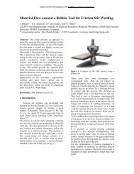
Figure 2. 3-D Model <strong>of</strong> the diaphragm<br />
4.2 Axisymmetric <strong>Synthetic</strong> Jet Actuator Model<br />
The results <strong>of</strong> the 3D model showed that the most<br />
relevant deformations occur in the z and radial<br />
directions. For these reasons and due to the<br />
<strong>com</strong>putational resources available, an<br />
axisymmetric model was implemented.<br />
4.2.1 Axisymmetric Disk <strong>Modeling</strong><br />
4.2.1.1 Subdomain Settings<br />
The Reynolds number is shown in equation (9):<br />
(9)<br />
<br />
Where U is a characteristic velocity <strong>of</strong> the flow (in<br />
the present work U is defined as the maximum<br />
instantaneous velocity i.e. U = max(u)), d is the<br />
diameter <strong>of</strong> the aperture. The Stokes Number is<br />
given by<br />
<br />
<br />
(10)<br />
Where is the oscillation frequency in rad/s, is<br />
the diameter <strong>of</strong> the aperture and is the kinematic<br />
viscosity <strong>of</strong> the fluid<br />
4. Models<br />
4.1 3-D Piezoelectric Disk <strong>Modeling</strong><br />
The first approach to the problem was to develop a<br />
3-D piezoelectric model <strong>of</strong> the diaphragm (Figure<br />
2). This model was tested at different voltages to<br />
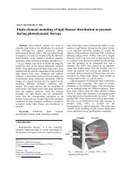
Figure 3. Geometry <strong>of</strong> the piezoelectric diaphragm.<br />
In Figure 3 the green area shows the<br />
piezoelectric material portion <strong>of</strong> the diaphragm<br />
while the gray area shows the metallic <strong>com</strong>ponent<br />
<strong>of</strong> the diaphragm.<br />
4.2.1.2 Boundary Settings<br />
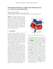
Figure 4 shows the boundaries used in the<br />
piezoelectric module, these are described in Table<br />
3. It is also assumed that there is no relative<br />
displacement between the piezoelectric and the<br />
metallic portions <strong>of</strong> the diaphragm. Boundaries 2,<br />
3, 4 and 7 are set free since these are the ones that<br />
move when the disk is excited. Boundary 1<br />
emulates the fixed side <strong>of</strong> the disk.
Figure 4. Numbering <strong>of</strong> the boundaries<br />
Table 3. Piezoelectric Disk Boundary Conditions<br />
Boundary Structural Electrical<br />
1 Fixed Continuity<br />
2 Free Continuity<br />
3 Free Continuity<br />
4 Free V0*sin(ωt)<br />
5 Axial Symmetry Continuity<br />
6 Axial Symmetry Continuity<br />
7 Free Continuity<br />
8 - Ground<br />
Where: V is the instant electric potential, V 0 is the<br />
electric potential’s amplitude. The diaphragm is<br />
designed for Electric Potentials between 0 and 500<br />
V, so the values chosen for V 0 are in this range.<br />
Since this is a low frequency study was fixed at<br />
2 rad/s.<br />
Figure 6. Whole Fluid subdomain.<br />
In Figures 5 and 6 the red area is the fluid<br />
subdomain. In Figure 6, the subdomain in the<br />
outside must be large enough so that the boundary<br />
conditions do not affect the <strong>Synthetic</strong> Jet, for this<br />
reason the horizontal edge <strong>of</strong> the outside domain is<br />
three times larger than the radius <strong>of</strong> the diaphragm<br />
while the vertical edge is five times this size.<br />
4.3.2 Boundary Settings<br />
Figures 7 and 8 show all the boundaries involved in<br />
the fluid model. Interior boundaries are not taken<br />
into account and all the boundaries <strong>of</strong> the disk are<br />
considered moving walls, which movement is<br />
determined by the deformation <strong>of</strong> the piezoelectric<br />
disk. Boundaries 13 and 14 are considered open.<br />
4.3 Axisymmetric Fluid Dynamics Model and<br />
Boundary Conditions<br />
4.3.1 Subdomain Settings<br />
The fluid subdomain includes all the fluid<br />
contained inside and outside the cavity. Though<br />
this is one subdomain, one can clearly distinguish<br />
between the fluid that is inside the cavity and the<br />
fluid outside.<br />
Figure 7. Fluid Boundaries Close-Up<br />
Figure 5. Fluid subdomain close-up.<br />
Figure 8. Fluid Boundaries
Table 4. Fluid Boundaries<br />
Boundary Fluid Boundary Fluid<br />
1 - 9 Wall<br />
2 Moving Wall 10 Wall<br />
3 Moving Wall 11 Wall<br />
4 Moving Wall 12 Wall<br />
5 Symmetry 13 Open<br />
6 Symmetry 14 Open<br />
7 - 15 Symmetry<br />
8 -<br />
5. Numerical Results<br />
5.1 3-D Piezoelectric Disk <strong>Modeling</strong><br />
The results <strong>of</strong> the 3D piezoelectric disk model are<br />
shown in Figure 9, in which the red triangles show<br />
the results <strong>of</strong> the numerical simulations, while the<br />
black dots and curve show the performance given<br />
by the manufacturer. It is observed that the<br />
experimental results tend to be linear while the<br />
black curve tends to be linear only under 300 V p-<br />
p. For this reason most <strong>of</strong> the experiments are<br />
performed in the range 0-300V p-p. The<br />
percentages in Figure 9 show the difference<br />
between the numerical simulations and the<br />
manufacturer experimental results. Between 0-<br />
300V the error is about 9% on average.<br />
Figure 10. Low 1/Sr at time 0.18.<br />
Figure 11. Low 1/Sr at Time 0.29.<br />
The vortex ring tries to escape from the aperture<br />
but instead it is swallowed again through the<br />
aperture as shown in Figure 11<br />
Figure 9. Displacement vs Voltage. (Face<br />
International Corporation, 2007)<br />
5.2 Low 1/Sr<br />
Figure 10 shows the moment when the vortex ring<br />
starts forming in the outside due to the outwards<br />
movement <strong>of</strong> the fluid inside the cavity.<br />
Figure 12. Low 1/Sr at Time 0.73.<br />
Figure 12 shows the swallowed vortex ring<br />
appearing inside the cavity as the fluid moves<br />
inwards.
5.3 High 1/Sr<br />
Figure 13. High 1/Sr at Time 0.02<br />
Figure 13 shows how; as the fluid flows outwards,<br />
a tiny vortex ring appears outside the cavity.<br />
Figure 14. High 1/Sr at Time 0.11.<br />
Figure 14 shows how the vortex ring escapes away<br />
from the aperture, so that it cannot be swallowed<br />
inside the cavity again and evolves as shown below<br />
(Figure 15)<br />
Figure 15. High 1/Sr at Time 0.16.<br />
6. Discussion<br />
Table 5 (Appendix 1) describes the results<br />
obtained in different experiments, for which<br />
different parameters where changed. Experiments<br />
1-3 show no significant change in the inverse <strong>of</strong> the<br />
Strouhal Number when varying the electric<br />
potential in one order <strong>of</strong> magnitude. For these<br />
experiments no jet formation is observed. For<br />
experiment 4 and 5 a change <strong>of</strong> one order <strong>of</strong><br />
magnitude was applied to the aperture’s diameter,<br />
afterwards two experiments in which the electric<br />
potential was varied were done, obtaining a<br />
significant increase in the inverse <strong>of</strong> the Strouhal<br />
Number, although no jet formation was observed.<br />
For this reason the diameter <strong>of</strong> the aperture will be<br />
held in the order <strong>of</strong> 10 -4 and other parameters<br />
changed. In experiments 8 to 11 the previous<br />
aperture’s size was maintained and the viscosity<br />
was varied, obtaining inverse Strouhal numbers<br />
greater than 100 and observing jet formation.<br />
7. Conclusions<br />
<br />
<br />
<br />
<br />
The fluid velocity is weakly dependant <strong>of</strong><br />
the applied voltage. Keeping in mind that the<br />
applied voltage must be only in a certain range<br />
(under 300 V), the model was proved for<br />
several voltages. When arriving near 300 V<br />
no significant increase was observed in the<br />
inverse <strong>of</strong> the Strouhal number. For this reason<br />
the voltage was increased even outside <strong>of</strong> the<br />
range (until 500 V) but no significant change<br />
was observed.<br />
The fluid velocity is strongly dependant <strong>of</strong><br />
the aperture diaphragm. When varying the<br />
aperture diaphragm dimension in one order <strong>of</strong><br />
magnitude, the inverse <strong>of</strong> the Strouhal number<br />
varies almost in two orders <strong>of</strong> magnitude.<br />
This is due to the mass conservation because<br />
through a smaller diameter the fluid will flow<br />
at a higher speed increasing the Reynolds<br />
Number and, thus, the Strouhal Number.<br />
The jet formation criterion for this problem<br />
is in the order <strong>of</strong> hundreds. After running<br />
several simulations <strong>of</strong> the model, it is seen that<br />
when the inverse <strong>of</strong> the Strouhal number is<br />
near one hundred a clear vortex formation and<br />
escape is differenced. An exact number can’t<br />
be given for this criterion since there exists<br />
always a transition zone between the jet and no<br />
jet formation.<br />
There exists vortex ring formation in the<br />
inside <strong>of</strong> the cavity. Never before, with the
classical one-physics simulations, an<br />
interaction <strong>of</strong> the vortex formation inside the<br />
cavity and the diaphragm has been observed.<br />
This is due to the diaphragm deformation and<br />
its wall condition, which makes the entering<br />
vortex to hit the diaphragm and start an<br />
interaction with it.<br />
8. Future Work<br />
<br />
<br />
<br />
<br />
<br />
<br />
Coupling <strong>of</strong> the acoustics module to the model<br />
Comparison with Lumped Element <strong>Modeling</strong><br />
results<br />
Study the influence <strong>of</strong> the vortex rings<br />
interactions with the diaphragm in the quality<br />
<strong>of</strong> SJ formation<br />
Study <strong>of</strong> the influence <strong>of</strong> the actuator’s height<br />
Study <strong>of</strong> the influence <strong>of</strong> the frequency in the<br />
SJ formation<br />
Study <strong>of</strong> the phenomena according to a<br />
turbulence model<br />
9. References<br />
1. Alan Barnett et al, Finite Element Approach to<br />
Model and Analyze Piezoelectric Actuators, JSME<br />
International Journal, 476-485 (2001)<br />
2. Quentin Gallas et al, Lumped Element <strong>Modeling</strong><br />
<strong>of</strong> Piezoelectric-Driven <strong>Synthetic</strong> Jet Actuators,<br />
AIAA Journal, 240-247 (2003)<br />
3. Ryan Holman, Formation Criterion for <strong>Synthetic</strong><br />
<strong>Jets</strong>, AIAA Journal, (2005)<br />
4. Uno Ingard, On the Theory and Design <strong>of</strong><br />
Acoustic Resonators, The Journal <strong>of</strong> the Acoustical<br />
Society <strong>of</strong> America, 1037-1061 (1953)<br />
5. Poorna Mane et al, Experimental design and<br />
analysis for piezoelectric circular actuators in flow<br />
control applications, Smart Materials and<br />
Structures (2008)<br />
7. Vincent Piefort, Finite Element Modelling <strong>of</strong><br />
Piezoelectric Active Structures, Ph.D. thesis.<br />
Bruxelles, Belgium: Université Libre de Bruxelles,<br />
Department for Mechanical Engineering and<br />
Robotics (2001)<br />
8. Christopher Rumsey, Proceedings <strong>of</strong> the 2004<br />
Workshop on CFD Validation <strong>of</strong> <strong>Synthetic</strong> <strong>Jets</strong> and<br />
Turbulent Separation Control, Hampton, Virginia:<br />
NASA. (2007)<br />
9. B. Smith et al, The Formation and Evolution <strong>of</strong><br />
<strong>Synthetic</strong> <strong>Jets</strong>, Physics <strong>of</strong> Fluids, 2281-2297 (1998)<br />
10. Yukata Takagi et al, Dielectric Properties <strong>of</strong><br />
Lead Zirconate, Journal <strong>of</strong> the Physical Society,<br />
208-209 (1951)<br />
11. David Durán et al, <strong>Computational</strong> <strong>Modeling</strong> <strong>of</strong><br />
<strong>Synthetic</strong> <strong>Jets</strong>, Mechanical Engineering Thesis<br />
(2010)<br />
10. Acknowledgements<br />
The authors would like to thank the<br />
Departments <strong>of</strong> Mechanical and Chemical<br />
Engineering <strong>of</strong> the Universidad de los Andes which<br />
financially supported this project.<br />
11. Appendix<br />
Table 5. Simulations Results Summary<br />
Exp.<br />
No.<br />
Diam.<br />
(m)<br />
height<br />
(m)<br />
Potential<br />
(V)<br />
viscosity<br />
(Pa.s)<br />
Vel max. (m/s) Reynolds Stokes 1/Sr Criterion<br />
1 2e-03 1.4e-03 25 1e-06 3.27e-03 6.54 5.01 0.26 no jet<br />
2 2e-03 1.4e-03 50 1e-06 3.27e-03 6.54 5.01 0.26 no jet<br />
3 2e-03 1.4e-03 200 1e-06 3.02e-03 6.05 5.01 0.24 no jet<br />
4 2e-04 1.4e-03 100 1e-06 1.21e-01 24.2 0.50 96.29 no jet<br />
5 2e-04 1.4e-03 500 1e-06 1.21e-01 24.2 0.50 96.29 no jet<br />
6 2e-04 1.4e-03 100 1e-07 0.135 270 1.59 107.43 jet<br />
7 2e-04 1.4e-03 100 1e-06 0.146 29.2 0.50 116.18 jet