FDWK_3ed_Ch05_pp262-319

Recommendations

Info

Chapter 5 Overview Section 5.1 Estimating with Finite Sums 263 The need to calculate instantaneous rates of change led the discoverers of calculus to an investigation of the slopes of tangent lines and, ultimately, to the derivative—to what we call differential calculus. But derivatives revealed only half the story. In addition to a calculation method (a “calculus”) to describe how functions change at any given instant, they needed a method to describe how those instantaneous changes could accumulate over an interval to produce the function. That is why they also investigated areas under curves, which ultimately led to the second main branch of calculus, called integral calculus. Once Newton and Leibniz had the calculus for finding slopes of tangent lines and the calculus for finding areas under curves—two geometric operations that would seem to have nothing at all to do with each other—the challenge for them was to prove the connection that they knew intuitively had to be there. The discovery of this connection (called the Fundamental Theorem of Calculus) brought differential and integral calculus together to become the single most powerful insight mathematicians had ever acquired for understanding how the universe worked. 5.1 What you’ll learn about • Distance Traveled • Rectangular Approximation Method (RAM) • Volume of a Sphere • Cardiac Output . . . and why Learning about estimating with finite sums sets the foundation for understanding integral calculus. Estimating with Finite Sums Distance Traveled We know why a mathematician pondering motion problems might have been led to consider slopes of curves, but what do those same motion problems have to do with areas under curves Consider the following problem from a typical elementary school textbook: A train moves along a track at a steady rate of 75 miles per hour from 7:00 A.M. to 9:00 A.M. What is the total distance traveled by the train Applying the well-known formula distance rate time, we find that the answer is 150 miles. Simple. Now suppose that you are Isaac Newton trying to make a connection between this formula and the graph of the velocity function. 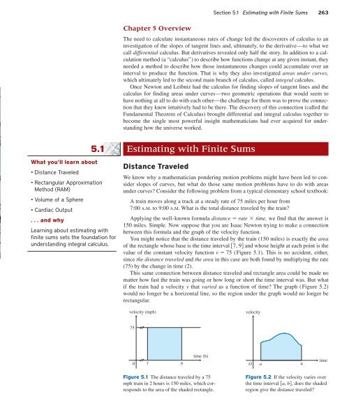You might notice that the distance traveled by the train (150 miles) is exactly the area of the rectangle whose base is the time interval 7, 9 and whose height at each point is the value of the constant velocity function v 75 (Figure 5.1). This is no accident, either, since the distance traveled and the area in this case are both found by multiplying the rate (75) by the change in time (2). This same connection between distance traveled and rectangle area could be made no matter how fast the train was going or how long or short the time interval was. But what if the train had a velocity v that varied as a function of time The graph (Figure 5.2) would no longer be a horizontal line, so the region under the graph would no longer be rectangular. velocity (mph) velocity 75 0 7 9 time (h) O a b time Figure 5.1 The distance traveled by a 75 mph train in 2 hours is 150 miles, which corresponds to the area of the shaded rectangle. Figure 5.2 If the velocity varies over the time interval a, b, does the shaded region give the distance traveled
264 Chapter 5 The Definite Integral Would the area of this irregular region still give the total distance traveled over the time interval Newton and Leibniz (and, actually, many others who had considered this question) thought that it obviously would, and that is why they were interested in a calculus for finding areas under curves. They imagined the time interval being partitioned into many tiny subintervals, each one so small that the velocity over it would essentially be constant. Geometrically, this was equivalent to slicing the irregular region into narrow strips, each of which would be nearly indistinguishable from a narrow rectangle (Figure 5.3). velocity O a b time Figure 5.3 The region is partitioned into vertical strips. If the strips are narrow enough, they are almost indistinguishable from rectangles. The sum of the areas of these “rectangles” will give the total area and can be interpreted as distance traveled. They argued that, just as the total area could be found by summing the areas of the (essentially rectangular) strips, the total distance traveled could be found by summing the small distances traveled over the tiny time intervals. EXAMPLE 1 Finding Distance Traveled when Velocity Varies A particle starts at x 0 and moves along the x-axis with velocity vt t 2 for time t 0. Where is the particle at t 3 SOLUTION We graph v and partition the time interval 0, 3 into subintervals of length Dt. (Figure 5.4 shows twelve subintervals of length 312 each.) v 9 v = t 2 v v t 2 0 1 2 3 t 0 0.5 0.75 1 Figure 5.5 The area of the shaded region is approximated by the area of the rectangle whose height is the function value at the midpoint of the interval. (Example 1) t Figure 5.4 The region under the parabola v t 2 from t 0 to t 3 is partitioned into 12 thin strips, each with base t 14. The strips have curved tops. (Example 1) Notice that the region under the curve is partitioned into thin strips with bases of length 14 and curved tops that slope upward from left to right. You might not know how to find the area of such a strip, but you can get a good approximation of it by finding the area of a suitable rectangle. In Figure 5.5, we use the rectangle whose height is the y-coordinate of the function at the midpoint of its base. continued
Page 1: Chapter 5 The Definite Integral The
Page 5 and 6: 266 Chapter 5 The Definite Integral
Page 53 and 54:
314 Chapter 5 The Definite Integral
Page 55 and 56:
Page 57 and 58:
show all

FDWK_3ed_Ch05_pp262-319

Create successful ePaper yourself

Delete template?

Save as template?