Fundamentals of Electric Circuits

c h a p t e r 

Methods of 

Analysis 

3 

No great work is ever done in a hurry. To develop a great scientific 

discovery, to print a great picture, to write an immortal poem, to 

become a minister, or a famous general—to do anything great requires 

time, patience, and perseverance. These things are done by degrees, 

“little by little.” 

—W. J. Wilmont Buxton 

Enhancing Your Career 

Career in Electronics 

One area of application for electric circuit analysis is electronics. The 

term electronics was originally used to distinguish circuits of very low 

current levels. This distinction no longer holds, as power semiconductor 

devices operate at high levels of current. Today, electronics is 

regarded as the science of the motion of charges in a gas, vacuum, or 

semiconductor. Modern electronics involves transistors and transistor 

circuits. The earlier electronic circuits were assembled from components. 

Many electronic circuits are now produced as integrated circuits, 

fabricated in a semiconductor substrate or chip. 

Electronic circuits find applications in many areas, such as automation, 

broadcasting, computers, and instrumentation. The range of devices 

that use electronic circuits is enormous and is limited only by our imagination. 

Radio, television, computers, and stereo systems are but a few. 

An electrical engineer usually performs diverse functions and is likely 

to use, design, or construct systems that incorporate some form of electronic 

circuits. Therefore, an understanding of the operation and analysis 

of electronics is essential to the electrical engineer. Electronics has 

become a specialty distinct from other disciplines within electrical engineering. 

Because the field of electronics is ever advancing, an electronics 

engineer must update his/her knowledge from time to time. The best way 

to do this is by being a member of a professional organization such as 

the Institute of Electrical and Electronics Engineers (IEEE). With a membership 

of over 300,000, the IEEE is the largest professional organization 

in the world. Members benefit immensely from the numerous magazines, 

journals, transactions, and conference/symposium proceedings published 

yearly by IEEE. You should consider becoming an IEEE member. 

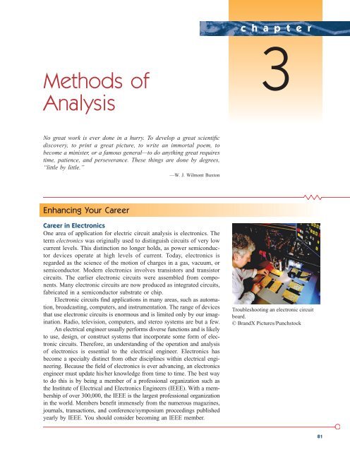
Troubleshooting an electronic circuit 

board. 

© BrandX Pictures/Punchstock 

81

82 Chapter 3 Methods of Analysis 

3.1 

Introduction 

Having understood the fundamental laws of circuit theory (Ohm’s law 

and Kirchhoff’s laws), we are now prepared to apply these laws to 

develop two powerful techniques for circuit analysis: nodal analysis, 

which is based on a systematic application of Kirchhoff’s current law 

(KCL), and mesh analysis, which is based on a systematic application 

of Kirchhoff’s voltage law (KVL). The two techniques are so important 

that this chapter should be regarded as the most important in the 

book. Students are therefore encouraged to pay careful attention. 

With the two techniques to be developed in this chapter, we can analyze 

any linear circuit by obtaining a set of simultaneous equations that 

are then solved to obtain the required values of current or voltage. One 

method of solving simultaneous equations involves Cramer’s rule, which 

allows us to calculate circuit variables as a quotient of determinants. The 

examples in the chapter will illustrate this method; Appendix A also 

briefly summarizes the essentials the reader needs to know for applying 

Cramer’s rule. Another method of solving simultaneous equations is to 

use MATLAB, a computer software discussed in Appendix E. 

Also in this chapter, we introduce the use of PSpice for Windows, 

a circuit simulation computer software program that we will use 

throughout the text. Finally, we apply the techniques learned in this 

chapter to analyze transistor circuits. 

Nodal analysis is also known as the 

node-voltage method. 

3.2 

Nodal Analysis 

Nodal analysis provides a general procedure for analyzing circuits 

using node voltages as the circuit variables. Choosing node voltages 

instead of element voltages as circuit variables is convenient and 

reduces the number of equations one must solve simultaneously. 

To simplify matters, we shall assume in this section that circuits 

do not contain voltage sources. Circuits that contain voltage sources 

will be analyzed in the next section. 

In nodal analysis, we are interested in finding the node voltages. 

Given a circuit with n nodes without voltage sources, the nodal analysis 

of the circuit involves taking the following three steps. 

Steps to Determine Node Voltages: 

1. Select a node as the reference node. Assign voltages v 1 , 

v 2 , p , v n1 to the remaining n 1 nodes. The voltages are 

referenced with respect to the reference node. 

2. Apply KCL to each of the n 1 nonreference nodes. Use 

Ohm’s law to express the branch currents in terms of node 

voltages. 

3. Solve the resulting simultaneous equations to obtain the 

unknown node voltages. 

We shall now explain and apply these three steps. 

The first step in nodal analysis is selecting a node as the reference 

or datum node. The reference node is commonly called the ground

3.2 Nodal Analysis 83 

since it is assumed to have zero potential. A reference node is indicated 

by any of the three symbols in Fig. 3.1. The type of ground in Fig. 3.1(c) 

is called a chassis ground and is used in devices where the case, enclosure, 

or chassis acts as a reference point for all circuits. When the 

potential of the earth is used as reference, we use the earth ground in 

Fig. 3.1(a) or (b). We shall always use the symbol in Fig. 3.1(b). 

Once we have selected a reference node, we assign voltage designations 

to nonreference nodes. Consider, for example, the circuit in 

Fig. 3.2(a). Node 0 is the reference node (v 0), while nodes 1 and 

2 are assigned voltages v 1 and v 2 , respectively. Keep in mind that the 

node voltages are defined with respect to the reference node. As illustrated 

in Fig. 3.2(a), each node voltage is the voltage rise from the reference 

node to the corresponding nonreference node or simply the 

voltage of that node with respect to the reference node. 

As the second step, we apply KCL to each nonreference node in 

the circuit. To avoid putting too much information on the same circuit, 

the circuit in Fig. 3.2(a) is redrawn in Fig. 3.2(b), where we now add 

i 1 , i 2 , and i 3 as the currents through resistors R 1 , R 2 , and respectively. 

At node 1, applying KCL gives 

I 1 I 2 i 1 i 2 

R 3 , 

(3.1) 

At node 2, 

I 2 i 2 i 3 

(3.2) 

We now apply Ohm’s law to express the unknown currents i 1 , i 2 , and 

i 3 in terms of node voltages. The key idea to bear in mind is that, since 

resistance is a passive element, by the passive sign convention, current 

must always flow from a higher potential to a lower potential. 

Current flows from a higher potential to a lower potential in a resistor. 

We can express this principle as 

i v higher v lower 

R 

(3.3) 

Note that this principle is in agreement with the way we defined resistance 

in Chapter 2 (see Fig. 2.1). With this in mind, we obtain from 

Fig. 3.2(b), 

i 1 v 1 0 

or i 1 G 1 v 1 

R 1 

i 2 v 1 v 2 

R 2 

or i 2 G 2 (v 1 v 2 ) 

i 3 v 2 0 

R 3 

or i 3 G 3 v 2 

Substituting Eq. (3.4) in Eqs. (3.1) and (3.2) results, respectively, in 

(3.4) 

The number of nonreference nodes is 

equal to the number of independent 

equations that we will derive. 

(a) (b) (c) 

Figure 3.1 

Common symbols for indicating a 

reference node, (a) common ground, 

(b) ground, (c) chassis ground. 

i 2 i 2 

v 1 

I 1 R 1 R 3 

I 2 

1 

R 2 2 

I 1 

+ 

v 1 R 1 

+ 

v 2 R 3 

− 

− 

0 

(a) 

I 2 

R 2 v 2 

i 1 

i 3 

(b) 

Figure 3.2 

Typical circuit for nodal analysis. 

I 1 I 2 v 1 

v 1 v 2 

R 1 R 2 

I 2 v 1 v 2 

v 2 

R 2 R 3 

(3.5) 

(3.6)


Appendix A discusses how to use 

Cramer’s rule. 

In terms of the conductances, Eqs. (3.5) and (3.6) become 

I 1 I 2 G 1 v 1 G 2 (v 1 v 2 ) 

(3.7) 

I 2 G 2 (v 1 v 2 ) G 3 v 2 

(3.8) 

The third step in nodal analysis is to solve for the node voltages. 

If we apply KCL to n 1 nonreference nodes, we obtain n 1 simultaneous 

equations such as Eqs. (3.5) and (3.6) or (3.7) and (3.8). For 

the circuit of Fig. 3.2, we solve Eqs. (3.5) and (3.6) or (3.7) and (3.8) 

to obtain the node voltages v 1 and v 2 using any standard method, such 

as the substitution method, the elimination method, Cramer’s rule, or 

matrix inversion. To use either of the last two methods, one must cast 

the simultaneous equations in matrix form. For example, Eqs. (3.7) and 

(3.8) can be cast in matrix form as 

c G 1 G 2 G 2 

d c v 1 

d c I 1 I 2 

d (3.9) 

G 2 G 2 G 3 v 2 I 2 

which can be solved to get v 1 and v 2 . Equation 3.9 will be generalized 

in Section 3.6. The simultaneous equations may also be solved using 

calculators or with software packages such as MATLAB, Mathcad, 

Maple, and Quattro Pro. 

Example 3.1 

Calculate the node voltages in the circuit shown in Fig. 3.3(a). 

5 A 

4 Ω 

1 

2 Ω 6 Ω 

2 

10 A 

Solution: 

Consider Fig. 3.3(b), where the circuit in Fig. 3.3(a) has been prepared 

for nodal analysis. Notice how the currents are selected for the 

application of KCL. Except for the branches with current sources, the 

labeling of the currents is arbitrary but consistent. (By consistent, we 

mean that if, for example, we assume that i 2 enters the 4- resistor 

from the left-hand side, i 2 must leave the resistor from the right-hand 

side.) The reference node is selected, and the node voltages v 1 and v 2 

are now to be determined. 

At node 1, applying KCL and Ohm’s law gives 

(a) 

i 1 i 2 i 3 1 5 v 1 v 2 

4 

v 1 0 

2 

5 A 

Multiplying each term in the last equation by 4, we obtain 

i 1 = 5 i 1 = 5 

v 1 

i 2 

i 

4 Ω 

4 = 10 

v 2 

i i 3 2 i5 

2 Ω 6 Ω 

10 A 

or 

At node 2, we do the same thing and get 

i 2 i 4 i 1 i 5 1 

20 v 1 v 2 2v 1 

3v 1 v 2 20 

Multiplying each term by 12 results in 

v 1 v 2 

4 

10 5 v 2 0 

6 

(3.1.1) 

(b) 

Figure 3.3 

For Example 3.1: (a) original circuit, 

(b) circuit for analysis. 

or 

3v 1 3v 2 120 60 2v 2 

3v 1 5v 2 60 

(3.1.2)


Now we have two simultaneous Eqs. (3.1.1) and (3.1.2). We can solve 

the equations using any method and obtain the values of and v 2 . 

■ METHOD 1 Using the elimination technique, we add Eqs. (3.1.1) 

and (3.1.2). 

Substituting v 2 20 in Eq. (3.1.1) gives 

■ METHOD 2 To use Cramer’s rule, we need to put Eqs. (3.1.1) 

and (3.1.2) in matrix form as 

The determinant of the matrix is 

3 1 

¢ ` ` 15 3 12 

3 5 

We now obtain v 1 and as 

v 2 

20 1 

v 1 ¢ ` 

1 

¢ 60 5 ` 

 

¢ 

3 20 

v 2 ¢ ` 

2 

¢ 3 60 ` 

 

¢ 

giving us the same result as did the elimination method. 

(3.1.3) 

If we need the currents, we can easily calculate them from the 

values of the nodal voltages. 

i 1 5 A, i 2 v 1 v 2 

4 

4v 2 80 1 v 2 20 V 

3v 1 20 20 1 v 1 40 

3 13.333 V 

3 1 

c 

3 5 d cv 1 

d c 20 

v 2 60 d 

100 60 

12 

180 60 

12 

13.333 V 

20 V 

1.6668 A, i 3 v 1 

2 6.666 A 

i 4 10 A, i 5 v 2 

6 3.333 A 

The fact that i 2 is negative shows that the current flows in the direction 

opposite to the one assumed. 

v 1 

Obtain the node voltages in the circuit of Fig. 3.4. 

Answer: v 1 2 V, v 2 14 V. 

Practice Problem 3.1 

1 6 Ω 2 

1 A 2 Ω 7 Ω 

4 A 

Figure 3.4 

For Practice Prob. 3.1.


Example 3.2 

Determine the voltages at the nodes in Fig. 3.5(a). 

Solution: 

The circuit in this example has three nonreference nodes, unlike the previous 

example which has two nonreference nodes. We assign voltages 

to the three nodes as shown in Fig. 3.5(b) and label the currents. 

4 Ω 

4 Ω 

i x 2 Ω 2 8 Ω 

1 3 

3 A 4 Ω 

2i x 

i 1 

i 

i 

2 Ω v 2 i 1 

8 Ω 2 

2 

v 1 v 3 

3 A i x i x 

i 3 

3 A 

4 Ω 

2i x 

0 

(a) 

Figure 3.5 

For Example 3.2: (a) original circuit, (b) circuit for analysis. 

At node 1, 

(b) 

Multiplying by 4 and rearranging terms, we get 

3v 1 2v 2 v 3 12 

At node 2, 

Multiplying by 8 and rearranging terms, we get 

4v 1 7v 2 v 3 0 

At node 3, 

3 i 1 i x 1 3 v 1 v 3 

4 

i x i 2 i 3 1 

i 1 i 2 2i x 1 

v 1 v 2 

2 

v 1 v 3 

4 

v 2 v 3 

8 

v 2 v 3 

8 

v 1 v 2 

2 

v 2 0 

4 

2(v 1 v 2 ) 

2 

(3.2.1) 

(3.2.2) 

Multiplying by 8, rearranging terms, and dividing by 3, we get 

2v 1 3v 2 v 3 0 

(3.2.3) 

We have three simultaneous equations to solve to get the node voltages 

v 1 , v 2 , and v 3 . We shall solve the equations in three ways. 

■ METHOD 1 Using the elimination technique, we add Eqs. (3.2.1) 

and (3.2.3). 

5v 1 5v 2 12 

or 

v 1 v 2 12 

(3.2.4) 

5 2.4 

Adding Eqs. (3.2.2) and (3.2.3) gives 

2v 1 4v 2 0 1 v 1 2v 2 (3.2.5)


Substituting Eq. (3.2.5) into Eq. (3.2.4) yields 

2v 2 v 2 2.4 1 v 2 2.4, v 1 2v 2 4.8 V 

From Eq. (3.2.3), we get 

Thus, 

■ METHOD 2 To use Cramer’s rule, we put Eqs. (3.2.1) to (3.2.3) 

in matrix form. 

From this, we obtain 

Similarly, we obtain 

¢ 1 

¢ 2 

 

 

 

 

 

 

¢ 3 

 

 

 

v 3 3v 2 2v 1 3v 2 4v 2 v 2 2.4 V 

v 1 4.8 V, v 2 2.4 V, v 3 2.4 V 

£ 

12 2 1 

0 7 1 

5 0 3 15 

12 2 1 

0 7 1 

3 12 1 

4 0 1 

5 2 0 15 

3 12 1 

4 0 1 

3 2 12 

4 7 0 

5 2 3 05 

3 2 12 

4 7 0 

3 2 1 

4 7 1 

2 3 1 

v 1 

§ £ v 2 § £ 

v 3 

12 

0 § 

0 

(3.2.6) 

v 1 ¢ 1 

¢ , v 2 ¢ 2 

¢ , v 3 ¢ 3 

¢ 

where ¢, ¢ 1 , ¢ 2 , and ¢ 3 are the determinants to be calculated as 

follows. As explained in Appendix A, to calculate the determinant of 

a 3 by 3 matrix, we repeat the first two rows and cross multiply. 

3 2 1 

3 2 1 4 7 1 

¢ 3 4 7 1 3 5 2 3 15 

2 3 1 3 2 1 

4 7 1 

 

 

21 12 4 14 9 8 10 

84 0 0 0 36 0 48 

 

 

 

0 0 24 0 0 48 24 

 

 

 

0 144 0 168 0 0 24


Thus, we find 

v 1 ¢ 1 

¢ 48 

10 4.8 V, v 2 ¢ 2 

¢ 24 

10 2.4 V 

as we obtained with Method 1. 

v 3 ¢ 3 

¢ 24 

10 2.4 V 

■ METHOD 3 We now use MATLAB to solve the matrix. Equation 

(3.2.6) can be written as 

AV B 1 V A 1 B 

where A is the 3 by 3 square matrix, B is the column vector, and V is 

a column vector comprised of v 1 , v 2 , and v 3 that we want to determine. 

We use MATLAB to determine V as follows: 

A [3 2 1; 4 7 1; 2 3 1]; 

B [12 0 0]; 

V inv(A) * B 

4.8000 

V 2.4000 

2.4000 

Thus, v 1 4.8 V, v 2 2.4 V, and v 3 2.4 V, as obtained previously. 

10 A 


2 Ω 

4i x 

3 Ω 2 

1 3 

i x 

Figure 3.6 

For Practice Prob. 3.2. 

4 Ω 6 Ω 

Find the voltages at the three nonreference nodes in the circuit of 

Fig. 3.6. 

Answer: v 1 80 V, v 2 64 V, v 3 156 V. 

3.3 

Nodal Analysis with Voltage Sources 

We now consider how voltage sources affect nodal analysis. We use the 

circuit in Fig. 3.7 for illustration. Consider the following two possibilities. 

■ CASE 1 If a voltage source is connected between the reference 

node and a nonreference node, we simply set the voltage at the nonreference 

node equal to the voltage of the voltage source. In Fig. 3.7, 

for example, 

v 1 10 V 

(3.10) 

Thus, our analysis is somewhat simplified by this knowledge of the voltage 

at this node. 

■ CASE 2 If the voltage source (dependent or independent) is connected 

between two nonreference nodes, the two nonreference nodes

3.3 Nodal Analysis with Voltage Sources 89 

10 V 

4 Ω 

Supernode 

i 4 

i 5 V 

2 Ω 1 

v 

v 2 1 v 3 

i 2 i 3 

+ − 

+ − 

8 Ω 6 Ω 

Figure 3.7 

A circuit with a supernode. 

form a generalized node or supernode; we apply both KCL and KVL 

to determine the node voltages. 

A supernode may be regarded as a 

closed surface enclosing the voltage 

source and its two nodes. 

A supernode is formed by enclosing a (dependent or independent) 

voltage source connected between two nonreference nodes and any 

elements connected in parallel with it. 

In Fig. 3.7, nodes 2 and 3 form a supernode. (We could have more 

than two nodes forming a single supernode. For example, see the circuit 

in Fig. 3.14.) We analyze a circuit with supernodes using the 

same three steps mentioned in the previous section except that the 

supernodes are treated differently. Why Because an essential component 

of nodal analysis is applying KCL, which requires knowing 

the current through each element. There is no way of knowing the 

current through a voltage source in advance. However, KCL must 

be satisfied at a supernode like any other node. Hence, at the supernode 

in Fig. 3.7, 

or 

v 1 v 2 

2 

i 1 i 4 i 2 i 3 

v 1 v 3 

4 

v 2 0 

8 

v 3 0 

6 

(3.11a) 

(3.11b) 

To apply Kirchhoff’s voltage law to the supernode in Fig. 3.7, we 

redraw the circuit as shown in Fig. 3.8. Going around the loop in the 

clockwise direction gives 

v 2 5 v 3 0 1 v 2 v 3 5 

From Eqs. (3.10), (3.11b), and (3.12), we obtain the node voltages. 

Note the following properties of a supernode: 

(3.12) 

1. The voltage source inside the supernode provides a constraint 

equation needed to solve for the node voltages. 

2. A supernode has no voltage of its own. 

3. A supernode requires the application of both KCL and KVL. 

5 V 

+ − 

+ + 

v 2 v 3 

Figure 3.8 

Applying KVL to a supernode. 

− 

−


2 A 

Example 3.3 

Figure 3.9 

For Example 3.3. 

2 V 

v 1 v 2 

2 Ω 

10 Ω 

+ − 

4 Ω 

7 A 

For the circuit shown in Fig. 3.9, find the node voltages. 

Solution: 

The supernode contains the 2-V source, nodes 1 and 2, and the 10- 

resistor. Applying KCL to the supernode as shown in Fig. 3.10(a) gives 

2 i 1 i 2 7 

Expressing i 1 and in terms of the node voltages 

or 

(3.3.1) 

To get the relationship between v 1 and v 2 , we apply KVL to the circuit 

in Fig. 3.10(b). Going around the loop, we obtain 

From Eqs. (3.3.1) and (3.3.2), we write 

or 

2 v 1 0 

2 

i 2 

v 2 0 

4 

7 1 8 2v 1 v 2 28 

v 2 20 2v 1 

v 1 2 v 2 0 1 v 2 v 1 2 

v 2 v 1 2 20 2v 1 

3v 1 22 1 v 1 7.333 V 

(3.3.2) 

and v 2 v 1 2 5.333 V. Note that the 10- 

resistor does not 

make any difference because it is connected across the supernode. 

2 A 

1 v 1 2 v 2 

i 1 i 2 

7 A 

2 V 

1 2 

+ 

+ − 

+ 

2 A 

2 Ω 4 Ω 

7 A 

v 1 v 2 

− 

− 

(a) 

Figure 3.10 

Applying: (a) KCL to the supernode, (b) KVL to the loop. 

(b) 

Practice Problem 3.3 Find v and i in the circuit of Fig. 3.11. 

4 Ω 

9 V 

Answer: 0.6 V, 4.2 A. 

21 V 

+ − 

+ − 

i 

+ 

3 Ω v 2 Ω 6 Ω 

− 

Figure 3.11 


3.3 Nodal Analysis with Voltage Sources 91 

Find the node voltages in the circuit of Fig. 3.12. Example 3.4 

3 Ω 

+ v x − 

20 V 

3v 

6 Ω 

x 

2 

1 + − + − 4 

2 Ω 10 A 

4 Ω 

1 Ω 

Figure 3.12 


Solution: 

Nodes 1 and 2 form a supernode; so do nodes 3 and 4. We apply KCL 

to the two supernodes as in Fig. 3.13(a). At supernode 1-2, 

i 3 10 i 1 i 2 

Expressing this in terms of the node voltages, 

or 

At supernode 3-4, 

v 3 v 2 

6 

10 v 1 v 4 

3 

v 1 

2 

5v 1 v 2 v 3 2v 4 60 

(3.4.1) 

or 

i 1 i 3 i 4 i 5 1 

v 1 v 4 

3 

v 3 v 2 

6 

4v 1 2v 2 5v 3 16v 4 0 

v 4 

1 v 3 

4 

(3.4.2) 

3 Ω 

+ v 

i x − 

1 

i 1 

6 Ω 

v 

v 2 v 3 1 v 4 

i i 

i 3 3 

2 i 5 i 4 

2 Ω 10 A 

4 Ω 1 Ω 

+ 

3 Ω 

v x − 

Loop 3 

20 V 

i 3 

3v x 

+ 

+ − 

+ − 

+ 

6 Ω 

+ 

+ 

v 1 Loop 1 v 2 v 3 Loop 2 v 4 

− − − − 

(a) 

Figure 3.13 

Applying: (a) KCL to the two supernodes, (b) KVL to the loops. 

(b)


We now apply KVL to the branches involving the voltage sources as 

shown in Fig. 3.13(b). For loop 1, 

v 1 20 v 2 0 1 v 1 v 2 20 

(3.4.3) 

For loop 2, 

v 3 3v x v 4 0 

But v x v 1 v 4 so that 

3v 1 v 3 2v 4 0 

(3.4.4) 

For loop 3, 

v x 3v x 6i 3 20 0 

But 6i 3 v 3 v 2 and v x v 1 v 4 . Hence, 

2v 1 v 2 v 3 2v 4 20 

(3.4.5) 

We need four node voltages, v 1 , v 2 , v 3 , and v 4 , and it requires only 

four out of the five Eqs. (3.4.1) to (3.4.5) to find them. Although the fifth 

equation is redundant, it can be used to check results. We can solve 

Eqs. (3.4.1) to (3.4.4) directly using MATLAB. We can eliminate one 

node voltage so that we solve three simultaneous equations instead of 

four. From Eq. (3.4.3), v 2 v 1 20. Substituting this into Eqs. (3.4.1) 

and (3.4.2), respectively, gives 

and 

6v 1 v 3 2v 4 80 

6v 1 5v 3 16v 4 40 

(3.4.6) 

(3.4.7) 

Equations (3.4.4), (3.4.6), and (3.4.7) can be cast in matrix form as 

Using Cramer’s rule gives 

3 1 2 v 1 0 

£ 6 1 2 § £ v 3 § £ 80 § 

6 5 16 v 4 40 

3 1 2 

0 1 2 

¢ † 6 1 2 † 18, ¢ 1 † 80 1 2 † 480, 

6 5 16 

40 5 16 

3 0 2 

3 1 0 

¢ 3 † 6 80 2 † 3120, ¢ 4 † 6 1 80 † 840 

6 40 16 

6 5 40 

Thus, we arrive at the node voltages as 

v 1 ¢ 1 

, 

¢ 480 

18 26.67 V, v 3 ¢ 3 

¢ 3120 

18 

173.33 V 

v 4 ¢ 4 

¢ 840 

18 46.67 V 

and v 2 v 1 20 6.667 V. We have not used Eq. (3.4.5); it can be 

used to cross check results.

3.4 Mesh Analysis 93 

Find v 1 , v 2 , and in the circuit of Fig. 3.14 using nodal analysis. 

v 3 

Answer: v 1 3.043 V, v 2 6.956 V, v 3 0.6522 V. 


6 Ω 

10 V 

v v 5i 

2 

1 + − 

v 3 

i 

+ − 

3.4 

Mesh Analysis 

Mesh analysis provides another general procedure for analyzing circuits, 

using mesh currents as the circuit variables. Using mesh currents 

instead of element currents as circuit variables is convenient and 

reduces the number of equations that must be solved simultaneously. 

Recall that a loop is a closed path with no node passed more than once. 

A mesh is a loop that does not contain any other loop within it. 

Nodal analysis applies KCL to find unknown voltages in a given 

circuit, while mesh analysis applies KVL to find unknown currents. 

Mesh analysis is not quite as general as nodal analysis because it is 

only applicable to a circuit that is planar. A planar circuit is one that 

can be drawn in a plane with no branches crossing one another; otherwise 

it is nonplanar. A circuit may have crossing branches and still 

be planar if it can be redrawn such that it has no crossing branches. 

For example, the circuit in Fig. 3.15(a) has two crossing branches, but 

it can be redrawn as in Fig. 3.15(b). Hence, the circuit in Fig. 3.15(a) 

is planar. However, the circuit in Fig. 3.16 is nonplanar, because there 

is no way to redraw it and avoid the branches crossing. Nonplanar circuits 

can be handled using nodal analysis, but they will not be considered 

in this text. 

2 Ω 4 Ω 3 Ω 

Figure 3.14 


Mesh analysis is also known as loop 

analysis or the mesh-current method. 

1 Ω 

1 A 

2 Ω 

5 Ω 6 Ω 

4 Ω 

3 Ω 

8 Ω 

7 Ω 

1 Ω 

(a) 

5 Ω 

6 Ω 

4 Ω 

3 Ω 

7 Ω 

2 Ω 

1 A 

2 Ω 

13 Ω 

5 A 

12 Ω 

11 Ω 

9 Ω 

8 Ω 

5 Ω 

1 Ω 3 Ω 

4 Ω 

6 Ω 

Figure 3.16 

A nonplanar circuit. 

10 Ω 

To understand mesh analysis, we should first explain more about 

what we mean by a mesh. 

8 Ω 7 Ω 

(b) 

Figure 3.15 

(a) A planar circuit with crossing branches, 

(b) the same circuit redrawn with no crossing 

branches. 

A mesh is a loop which does not contain any other loops within it.


a 

I 1 R1 

b 

I 2 R 2 c 

I 3 

V 1 

+ − 

i 1 

R 3 

i 2 

+ − V 2 

f 

Figure 3.17 

A circuit with two meshes. 

e 

d 

Although path abcdefa is a loop and 

not a mesh, KVL still holds. This is the 

reason for loosely using the terms 

loop analysis and mesh analysis to 

mean the same thing. 

In Fig. 3.17, for example, paths abefa and bcdeb are meshes, but path 

abcdefa is not a mesh. The current through a mesh is known as mesh 

current. In mesh analysis, we are interested in applying KVL to find 

the mesh currents in a given circuit. 

In this section, we will apply mesh analysis to planar circuits that 

do not contain current sources. In the next section, we will consider 

circuits with current sources. In the mesh analysis of a circuit with n 

meshes, we take the following three steps. 

Steps to Determine Mesh Currents: 

1. Assign mesh currents i 1 , i 2 , p , i n to the n meshes. 

2. Apply KVL to each of the n meshes. Use Ohm’s law to 

express the voltages in terms of the mesh currents. 

3. Solve the resulting n simultaneous equations to get the mesh 

currents. 

The direction of the mesh current is 

arbitrary—(clockwise or counterclockwise)—and 

does not affect the validity 

of the solution. 

The shortcut way will not apply if one 

mesh current is assumed clockwise 

and the other assumed counterclockwise, 

although this is permissible. 

To illustrate the steps, consider the circuit in Fig. 3.17. The first 

step requires that mesh currents i 1 and i 2 are assigned to meshes 1 and 

2. Although a mesh current may be assigned to each mesh in an arbitrary 

direction, it is conventional to assume that each mesh current 

flows clockwise. 

As the second step, we apply KVL to each mesh. Applying KVL 

to mesh 1, we obtain 

or 

For mesh 2, applying KVL gives 

or 

V 1 R 1 i 1 R 3 (i 1 i 2 ) 0 

(R 1 R 3 ) i 1 R 3 i 2 V 1 

R 2 i 2 V 2 R 3 (i 2 i 1 ) 0 

R 3 i 1 (R 2 R 3 )i 2 V 2 

(3.13) 

(3.14) 

Note in Eq. (3.13) that the coefficient of i 1 is the sum of the resistances 

in the first mesh, while the coefficient of i 2 is the negative of the resistance 

common to meshes 1 and 2. Now observe that the same is true 

in Eq. (3.14). This can serve as a shortcut way of writing the mesh 

equations. We will exploit this idea in Section 3.6.


The third step is to solve for the mesh currents. Putting Eqs. (3.13) 

and (3.14) in matrix form yields 

(3.15) 

which can be solved to obtain the mesh currents i 1 and i 2 . We are at 

liberty to use any technique for solving the simultaneous equations. 

According to Eq. (2.12), if a circuit has n nodes, b branches, and l independent 

loops or meshes, then l b n 1. Hence, l independent 

simultaneous equations are required to solve the circuit using mesh 

analysis. 

Notice that the branch currents are different from the mesh currents 

unless the mesh is isolated. To distinguish between the two types 

of currents, we use i for a mesh current and I for a branch current. The 

current elements I 1 , I 2 , and I 3 are algebraic sums of the mesh currents. 

It is evident from Fig. 3.17 that 

V 1 

c R 1 R 3 R 3 

d c i 1 

d c d 

R 3 R 2 R 3 i 2 V 2 

I 1 i 1 , I 2 i 2 , I 3 i 1 i 2 

(3.16) 

For the circuit in Fig. 3.18, find the branch currents and I 3 using 

mesh analysis. 

Solution: 

We first obtain the mesh currents using KVL. For mesh 1, 

or 

For mesh 2, 

or 

15 5i 1 10(i 1 i 2 ) 10 0 

3i 1 2i 2 1 

6i 2 4i 2 10(i 2 i 1 ) 10 0 

i 1 2i 2 1 

I 1 , I 2 , Example 3.5 

(3.5.1) 

(3.5.2) 

15 V 

I 1 I 2 5 Ω 6 Ω 

I 3 

10 Ω 

i 1 i 2 

+ − 

+ − 

Figure 3.18 


10 V 

4 Ω 

■ METHOD 1 Using the substitution method, we substitute 

Eq. (3.5.2) into Eq. (3.5.1), and write 

6i 2 3 2i 2 1 1 i 2 1 A 

From Eq. (3.5.2), i 1 2i 2 1 2 1 1 A. Thus, 

I 1 i 1 1 A, I 2 i 2 1 A, I 3 i 1 i 2 0 

■ METHOD 2 To use Cramer’s rule, we cast Eqs. (3.5.1) and 

(3.5.2) in matrix form as 

3 2 

c 

1 2 d ci 1 

d c 1 i 2 1 d


We obtain the determinants 

Thus, 

¢ 1 2 

1 ` 

1 2 ` 2 2 4, 

3 2 

¢ ` 

1 2 ` 6 2 4 

3 1 

¢ 2 ` 

1 1 ` 3 1 4 

as before. 

i 1 ¢ 1 

¢ 1 A, i 2 ¢ 2 

¢ 1 A 


i 1 

Calculate the mesh currents and of the circuit of Fig. 3.19. 

i 2 

Answer: i 1 2 A, i 2 0 A. 

2 Ω 

9 Ω 

12 Ω 

36 V + i 1 + − 24 V 

i − 2 

4 Ω 3 Ω 

Figure 3.19 


Example 3.6 

Use mesh analysis to find the current in the circuit of Fig. 3.20. 

I o 

24 V 

i 2 i 1 

A 

I o 

10 Ω 

i 2 

24 Ω 

4 Ω 

12 Ω i 3 

+ 

− 

+ − 

i 1 

Figure 3.20 


4I o 

Solution: 

We apply KVL to the three meshes in turn. For mesh 1, 

or 

For mesh 2, 

or 

For mesh 3, 

24 10 (i 1 i 2 ) 12 (i 1 i 3 ) 0 

11i 1 5i 2 6i 3 12 

24i 2 4 (i 2 i 3 ) 10 (i 2 i 1 ) 0 

5i 1 19i 2 2i 3 0 

4I o 12(i 3 i 1 ) 4(i 3 i 2 ) 0 

(3.6.1) 

(3.6.2)


But at node A, I o i 1 i 2 , so that 

4(i 1 i 2 ) 12(i 3 i 1 ) 4(i 3 i 2 ) 0 

or 

i 1 i 2 2i 3 0 

(3.6.3) 

In matrix form, Eqs. (3.6.1) to (3.6.3) become 

We obtain the determinants as 

¢ 

418 30 10 114 22 50 192 

12 5 6 

0 19 2 

¢ 1 5 0 1 25 

456 24 432 

12 5 6 

 

 

0 19 2 

 

¢ 2 

¢ 3 

 

 

 

 

 

 

 

 

 

11 5 6 

£ 5 19 2 

1 1 2 

11 5 12 

5 19 0 

5 1 1 05 

11 5 12 

5 19 0 

We calculate the mesh currents using Cramer’s rule as 

i 1 ¢ 1 

, 

¢ 432 

192 2.25 A, i 2 ¢ 2 

¢ 144 

192 0.75 A 

Thus, I o i 1 i 2 1.5 A. 

11 5 6 

5 19 2 

5 1 1 25 

11 5 6 

5 19 2 

11 12 6 

5 0 2 

5 1 0 25 

11 12 6 

5 0 2 

i 1 

§ £ i 2 § £ 

i 3 

 

 

 

i 3 ¢ 3 

¢ 288 

192 1.5 A 

12 

0 § 

0 

24 120 144 

 

 

 

60 228 288



6 Ω 

Using mesh analysis, find in the circuit of Fig. 3.21. 

Answer: 5 A. 

I o 

I o 

i 3 

4 Ω 8 Ω 

20 V 

+ – − 2 Ω 

i + 

1 i 2 

Figure 3.21 


10i o 

3.5 

Mesh Analysis with Current Sources 

Applying mesh analysis to circuits containing current sources (dependent 

or independent) may appear complicated. But it is actually much easier 

than what we encountered in the previous section, because the presence 

of the current sources reduces the number of equations. Consider the 

following two possible cases. 

10 V 

4 Ω 3 Ω 

+ − i 1 6 Ω i 2 5 A 

■ CASE 1 When a current source exists only in one mesh: Consider 

the circuit in Fig. 3.22, for example. We set i 2 5 A and write a 

mesh equation for the other mesh in the usual way; that is, 

10 4i 1 6(i 1 i 2 ) 0 1 i 1 2 A (3.17) 

Figure 3.22 

A circuit with a current source. 

■ CASE 2 When a current source exists between two meshes: Consider 

the circuit in Fig. 3.23(a), for example. We create a supermesh 

by excluding the current source and any elements connected in series 

with it, as shown in Fig. 3.23(b). Thus, 

A supermesh results when two meshes have a (dependent or independent) 

current source in common. 

6 Ω 10 Ω 

6 Ω 10 Ω 

2 Ω 

20 V 

+ − 

i 1 i 2 

6 A 

i 2 

4 Ω 

20 V + i 1 i − 

2 4 Ω 

i 1 

0 

Exclude these 

(b) 

(a) 

elements 

Figure 3.23 

(a) Two meshes having a current source in common, (b) a supermesh, created by excluding the current 

source. 

As shown in Fig. 3.23(b), we create a supermesh as the periphery of 

the two meshes and treat it differently. (If a circuit has two or more 

supermeshes that intersect, they should be combined to form a larger 

supermesh.) Why treat the supermesh differently Because mesh analysis 

applies KVL—which requires that we know the voltage across each 

branch—and we do not know the voltage across a current source in 

advance. However, a supermesh must satisfy KVL like any other mesh. 

Therefore, applying KVL to the supermesh in Fig. 3.23(b) gives 

20 6i 1 10i 2 4i 2 0

3.5 Mesh Analysis with Current Sources 99 

or 

6i 1 14i 2 20 

(3.18) 

We apply KCL to a node in the branch where the two meshes intersect. 

Applying KCL to node 0 in Fig. 3.23(a) gives 

i 2 i 1 6 

Solving Eqs. (3.18) and (3.19), we get 

i 1 3.2 A, i 2 2.8 A 

Note the following properties of a supermesh: 

(3.19) 

(3.20) 

1. The current source in the supermesh provides the constraint equation 

necessary to solve for the mesh currents. 

2. A supermesh has no current of its own. 

3. A supermesh requires the application of both KVL and KCL. 

For the circuit in Fig. 3.24, find i 1 to i 4 using mesh analysis. 

Example 3.7 

2 Ω 

i 1 

i 1 

4 Ω 

2 Ω 

P 

i 2 5 A 

I o 

i 2 i 3 

6 Ω i 2 3I o i 3 8 Ω i 4 

+ − 10 V 

Q 

Figure 3.24 


Solution: 

Note that meshes 1 and 2 form a supermesh since they have an 

independent current source in common. Also, meshes 2 and 3 form 

another supermesh because they have a dependent current source in 

common. The two supermeshes intersect and form a larger supermesh 

as shown. Applying KVL to the larger supermesh, 

or 

2i 1 4i 3 8(i 3 i 4 ) 6i 2 0 

i 1 3i 2 6i 3 4i 4 0 

For the independent current source, we apply KCL to node P: 

i 2 i 1 5 

For the dependent current source, we apply KCL to node Q: 

(3.7.1) 

(3.7.2) 

i 2 i 3 3I o


But I o i 4 , hence, 

i 2 i 3 3i 4 

(3.7.3) 

Applying KVL in mesh 4, 

2i 4 8(i 4 i 3 ) 10 0 

or 

5i 4 4i 3 5 

(3.7.4) 

From Eqs. (3.7.1) to (3.7.4), 

i 1 7.5 A, i 2 2.5 A, i 3 3.93 A, i 4 2.143 A 


Use mesh analysis to determine i 1 , i 2 , and in Fig. 3.25. 

i 3 

6 V 

2 Ω 2 Ω 

+ − 

4 Ω 

3 A 

i 1 

i 3 

Answer: i 1 3.474 A, i 2 0.4737 A, i 3 1.1052 A. 

1 Ω 

Figure 3.25 


G 2 

i 2 

I 2 

v 2 

8 Ω 

3.6 

Nodal and Mesh Analyses 

by Inspection 

This section presents a generalized procedure for nodal or mesh analysis. 

It is a shortcut approach based on mere inspection of a circuit. 

When all sources in a circuit are independent current sources, we 

do not need to apply KCL to each node to obtain the node-voltage 

equations as we did in Section 3.2. We can obtain the equations by 

mere inspection of the circuit. As an example, let us reexamine the circuit 

in Fig. 3.2, shown again in Fig. 3.26(a) for convenience. The 

circuit has two nonreference nodes and the node equations were 

derived in Section 3.2 as 

v 1 

I 1 G 1 G 3 

(a) 

R 1 R 2 

V 1 + − i 1 R 3 i 3 

+ − V 2 

c G 1 G 2 G 2 

d c v 1 

d c I 1 I 2 

d 

G 2 G 2 G 3 v 2 

(3.21) 

Observe that each of the diagonal terms is the sum of the conductances 

connected directly to node 1 or 2, while the off-diagonal terms are the 

negatives of the conductances connected between the nodes. Also, each 

term on the right-hand side of Eq. (3.21) is the algebraic sum of the 

currents entering the node. 

In general, if a circuit with independent current sources has N nonreference 

nodes, the node-voltage equations can be written in terms of 

the conductances as 

I 2 

(b) 

Figure 3.26 

(a) The circuit in Fig. 3.2, (b) the circuit 

in Fig. 3.17. 

≥ 

G 11 G 12 p G 1N 

G 21 G 22 p G 2N 

¥ ≥ 

o o o o 

G N1 G N2 p G NN 

v 1 

v 2 

i 1 

i 2 

¥ ≥ ¥ 

o o 

v N i N 

(3.22)

3.6 Nodal and Mesh Analyses by Inspection 101 

or simply 

Gv i 

(3.23) 

where 

G kk Sum of the conductances connected to node k 

G k j G jk Negative of the sum of the conductances directly 

connecting nodes k and j, k j 

v k Unknown voltage at node k 

i k Sum of all independent current sources directly connected 

to node k, with currents entering the node treated as positive 

G is called the conductance matrix; v is the output vector; and i is the 

input vector. Equation (3.22) can be solved to obtain the unknown node 

voltages. Keep in mind that this is valid for circuits with only independent 

current sources and linear resistors. 

Similarly, we can obtain mesh-current equations by inspection 

when a linear resistive circuit has only independent voltage sources. 

Consider the circuit in Fig. 3.17, shown again in Fig. 3.26(b) for convenience. 

The circuit has two nonreference nodes and the node equations 

were derived in Section 3.4 as 

v 1 

c R 1 R 3 R 3 

d c i 1 

d c d 

R 3 R 2 R 3 i 2 v 2 

(3.24) 

We notice that each of the diagonal terms is the sum of the resistances 

in the related mesh, while each of the off-diagonal terms is the negative 

of the resistance common to meshes 1 and 2. Each term on the 

right-hand side of Eq. (3.24) is the algebraic sum taken clockwise of 

all independent voltage sources in the related mesh. 

In general, if the circuit has N meshes, the mesh-current equations 

can be expressed in terms of the resistances as 

≥ 

R 11 R 12 p R 1N 

R 21 R 22 p R 2N 

¥ ≥ 

o o o o 

R N1 R N2 p R NN 

i 1 

v 1 

i 2 v 2 

¥ ≥ ¥ 

o o 

i N v N 

(3.25) 

or simply 

Ri v 

(3.26) 

where 

R kk Sum of the resistances in mesh k 

R kj R jk Negative of the sum of the resistances in common 

with meshes k and j, k j 

i k Unknown mesh current for mesh k in the clockwise direction 

v k Sum taken clockwise of all independent voltage sources in 

mesh k, with voltage rise treated as positive 

R is called the resistance matrix; i is the output vector; and v is 

the input vector. We can solve Eq. (3.25) to obtain the unknown mesh 

currents.


Example 3.8 

Write the node-voltage matrix equations for the circuit in Fig. 3.27 by 

inspection. 

2 A 

1 Ω 

v 1 5 Ω v 2 8 Ω v 3 8 Ω v 4 

3 A 10 Ω 1 A 4 Ω 2 Ω 

4 A 

Figure 3.27 


Solution: 

The circuit in Fig. 3.27 has four nonreference nodes, so we need four 

node equations. This implies that the size of the conductance matrix 

G, is 4 by 4. The diagonal terms of G, in siemens, are 

G 11 1 5 1 

10 0.3, G 22 1 5 1 8 1 1 1.325 

G 33 1 8 1 8 1 4 0.5, G 44 1 8 1 2 1 1 1.625 

The off-diagonal terms are 

G 12 1 5 0.2, G 13 G 14 0 

G 21 0.2, G 23 1 8 0.125, G 24 1 1 1 

G 31 0, G 32 0.125, G 34 1 8 0.125 

G 41 0, G 42 1, G 43 0.125 

The input current vector i has the following terms, in amperes: 

i 1 3, i 2 1 2 3, i 3 0, i 4 2 4 6 

Thus the node-voltage equations are 

0.3 0.2 0 0 v 1 3 

0.2 1.325 0.125 1 v 2 3 

≥ 

¥ ≥ ¥ ≥ ¥ 

0 0.125 0.5 0.125 v 3 0 

0 1 0.125 1.625 v 4 6 

which can be solved using MATLAB to obtain the node voltages 

v 3 , and v 4 . 

v 1 , v 2 ,

3.6 Nodal and Mesh Analyses by Inspection 103 

By inspection, obtain the node-voltage equations for the circuit in 

Fig. 3.28. 

Answer: 

1.3 0.2 1 0 v 1 

0.2 0.2 0 0 v 2 

≥ 

¥ ≥ ¥ ≥ 

1 0 1.25 0.25 v 3 

0 0 0.25 0.75 v 4 

0 

3 

¥ 

1 

3 


1 Ω v 3 4 Ω v 4 

1 A 

v 1 

5 Ω 

v 2 2 Ω 

10 Ω 

2 A 

3 A 

Figure 3.28 


By inspection, write the mesh-current equations for the circuit in Fig. 3.29. Example 3.9 

5 Ω 

i 1 

2 Ω 

4 V 

+ − 

2 Ω 

2 Ω 

10 V 

+ − 

1 Ω 1 Ω 

i 2 4 Ω 

i 3 

3 Ω 

4 Ω 

i 3 Ω 

+ 4 i 5 − 6 V 

+ − 

12 V 

Figure 3.29 


Solution: 

We have five meshes, so the resistance matrix is 5 by 5. The diagonal 

terms, in ohms, are: 

R 11 5 2 2 9, R 22 2 4 1 1 2 10, 

R 33 2 3 4 9, R 44 1 3 4 8, R 55 1 3 4 

The off-diagonal terms are: 

R 12 2, R 13 2, R 14 0 R 15 , 

R 21 2, R 23 4, R 24 1, R 25 1, 

R 31 2, R 32 4, R 34 0 R 35 , 

R 41 0, R 42 1, R 43 0, R 45 3, 

R 51 0, R 52 1, R 53 0, R 54 3 

The input voltage vector v has the following terms in volts: 

v 1 4, v 2 10 4 6, 

v 3 12 6 6, v 4 0, v 5 6


Thus, the mesh-current equations are: 

9 2 2 0 0 

2 10 4 1 1 

E2 4 9 0 0U 

0 1 0 8 3 

0 1 0 3 4 

i 1 4 

i 2 6 

Ei 3 U E6U 

i 4 0 

i 5 6 

From this, we can use MATLAB to obtain mesh currents 

and i 5 . 

i 1 , i 2 , i 3 , i 4 , 


By inspection, obtain the mesh-current equations for the circuit in 

Fig. 3.30. 

50 Ω 

40 Ω 

30 Ω 

+ − 

12 V 

24 V 

i 2 i 3 

10 Ω 

20 Ω 

i 1 

+ − 

+ − 

i 4 i 5 

80 Ω 

10 V 

60 Ω 

Figure 3.30 


Answer: 

170 40 0 80 0 

40 80 30 10 0 

E 0 30 50 0 20U 

80 10 0 90 0 

0 0 20 0 80 

i 1 24 

i 2 0 

Ei 3 U E12U 

i 4 10 

i 5 10 

3.7 

Nodal Versus Mesh Analysis 

Both nodal and mesh analyses provide a systematic way of analyzing 

a complex network. Someone may ask: Given a network to be analyzed, 

how do we know which method is better or more efficient The 

choice of the better method is dictated by two factors.

3.8 Circuit Analysis with PSpice 105 

The first factor is the nature of the particular network. Networks 

that contain many series-connected elements, voltage sources, or supermeshes 

are more suitable for mesh analysis, whereas networks with 

parallel-connected elements, current sources, or supernodes are more 

suitable for nodal analysis. Also, a circuit with fewer nodes than 

meshes is better analyzed using nodal analysis, while a circuit with 

fewer meshes than nodes is better analyzed using mesh analysis. The 

key is to select the method that results in the smaller number of 

equations. 

The second factor is the information required. If node voltages are 

required, it may be expedient to apply nodal analysis. If branch or mesh 

currents are required, it may be better to use mesh analysis. 

It is helpful to be familiar with both methods of analysis, for at 

least two reasons. First, one method can be used to check the results 

from the other method, if possible. Second, since each method has its 

limitations, only one method may be suitable for a particular problem. 

For example, mesh analysis is the only method to use in analyzing transistor 

circuits, as we shall see in Section 3.9. But mesh analysis cannot 

easily be used to solve an op amp circuit, as we shall see in Chapter 5, 

because there is no direct way to obtain the voltage across the op amp 

itself. For nonplanar networks, nodal analysis is the only option, 

because mesh analysis only applies to planar networks. Also, nodal 

analysis is more amenable to solution by computer, as it is easy to program. 

This allows one to analyze complicated circuits that defy hand 

calculation. A computer software package based on nodal analysis is 

introduced next. 

3.8 

Circuit Analysis with PSpice 

PSpice is a computer software circuit analysis program that we will 

gradually learn to use throughout the course of this text. This section 

illustrates how to use PSpice for Windows to analyze the dc circuits we 

have studied so far. 

The reader is expected to review Sections D.1 through D.3 of 

Appendix D before proceeding in this section. It should be noted that 

PSpice is only helpful in determining branch voltages and currents 

when the numerical values of all the circuit components are known. 

Appendix D provides a tutorial on 

using PSpice for Windows. 

Use PSpice to find the node voltages in the circuit of Fig. 3.31. 

Solution: 

The first step is to draw the given circuit using Schematics. If one 

follows the instructions given in Appendix sections D.2 and D.3, the 

schematic in Fig. 3.32 is produced. Since this is a dc analysis, we use 

voltage source VDC and current source IDC. The pseudocomponent 

VIEWPOINTS are added to display the required node voltages. Once 

the circuit is drawn and saved as exam310.sch, we run PSpice by 

selecting Analysis/Simulate. The circuit is simulated and the results 

120 V 

Example 3.10 

1 20 Ω 2 10 Ω 3 

+ − 30 Ω 40 Ω 3 A 

0 

Figure 3.31 

For Example 3.10.


120.0000 R1 

R3 

1 2 3 

20 10 

+ 

120 V V 1 R2 30 R4 40 I1 

IDC 

3 A 

− 

0 

Figure 3.32 

For Example 3.10; the schematic of the circuit in Fig. 3.31. 

are displayed on VIEWPOINTS and also saved in output file 

exam310.out. The output file includes the following: 

NODE VOLTAGE NODE VOLTAGE NODE VOLTAGE 

(1) 120.0000 (2) 81.2900 (3) 89.0320 

indicating that V 1 120 V, V 2 81.29 V, V 3 89.032 V. 


For the circuit in Fig. 3.33, use PSpice to find the node voltages. 

2 A 

1 2 100 Ω 3 

30 Ω 60 Ω 50 Ω 

25 Ω 

+ − 

200 V 

Figure 3.33 


0 

Answer: V 1 40 V, V 2 57.14 V, V 3 200 V. 

Example 3.11 

In the circuit of Fig. 3.34, determine the currents i 1 , i 2 , and i 3 . 

1 Ω 

24 V 

+ − 

4 Ω 2 Ω 

3v o 

+ − 

i 1 i 2 i 3 

2 Ω 8 Ω 4 Ω 

+ 

v o 

− 

Figure 3.34 

For Example 3.11.

3.9 Applications: DC Transistor Circuits 107 

Solution: 

The schematic is shown in Fig. 3.35. (The schematic in Fig. 3.35 

includes the output results, implying that it is the schematic displayed 

on the screen after the simulation.) Notice that the voltage-controlled 

voltage source E1 in Fig. 3.35 is connected so that its input is the 

voltage across the 4- 

resistor; its gain is set equal to 3. In order to 

display the required currents, we insert pseudocomponent IPROBES in 

the appropriate branches. The schematic is saved as exam311.sch and 

simulated by selecting Analysis/Simulate. The results are displayed on 

IPROBES as shown in Fig. 3.35 and saved in output file exam311.out. 

From the output file or the IPROBES, we obtain i 1 i 2 1.333 A and 

i 3 2.667 A. 

2 

R5 

E 

− + 

− + 

E1 

R1 

4 

+ 

24 V V 1 

− 

1 

R6 

R2 2 R3 8 R4 4 

1.333E + 00 1.333E + 00 2.667E + 00 

0 

Figure 3.35 

The schematic of the circuit in Fig. 3.34. 

i 1 , i 2 , Practice Problem 3.11 

Use PSpice to determine currents and in the circuit of Fig. 3.36. 

i 3 

Answer: i 1 0.4286 A, i 2 2.286 A, i 3 2 A. 

3.9 

Applications: DC Transistor Circuits 

Most of us deal with electronic products on a routine basis and have 

some experience with personal computers. A basic component for 

the integrated circuits found in these electronics and computers is the 

active, three-terminal device known as the transistor. Understanding 

the transistor is essential before an engineer can start an electronic circuit 

design. 

Figure 3.37 depicts various kinds of transistors commercially available. 

There are two basic types of transistors: bipolar junction transistors 

(BJTs) and field-effect transistors (FETs). Here, we consider only 

the BJTs, which were the first of the two and are still used today. Our 

objective is to present enough detail about the BJT to enable us to apply 

the techniques developed in this chapter to analyze dc transistor circuits. 

2 Ω 

10 V 

i 1 

+ − 

4 Ω 

2 A 

i 2 

i 3 

1 Ω i 1 2 Ω 

Figure 3.36 



Historical 

Courtesy of Lucent 

Technologies/Bell Labs 

William Schockley (1910–1989), John Bardeen (1908–1991), and 

Walter Brattain (1902–1987) co-invented the transistor. 

Nothing has had a greater impact on the transition from the “Industrial 

Age” to the “Age of the Engineer” than the transistor. I am sure 

that Dr. Shockley, Dr. Bardeen, and Dr. Brattain had no idea they would 

have this incredible effect on our history. While working at Bell Laboratories, 

they successfully demonstrated the point-contact transistor, 

invented by Bardeen and Brattain in 1947, and the junction transistor, 

which Shockley conceived in 1948 and successfully produced in 1951. 

It is interesting to note that the idea of the field-effect transistor, 

the most commonly used one today, was first conceived in 1925–1928 

by J. E. Lilienfeld, a German immigrant to the United States. This is 

evident from his patents of what appears to be a field-effect transistor. 

Unfortunately, the technology to realize this device had to wait until 

1954 when Shockley’s field-effect transistor became a reality. Just think 

what today would be like if we had this transistor 30 years earlier! 

For their contributions to the creation of the transistor, Dr. Shockley, 

Dr. Bardeen, and Dr. Brattain received, in 1956, the Nobel Prize in 

physics. It should be noted that Dr. Bardeen is the only individual to 

win two Nobel prizes in physics; the second came later for work in 

superconductivity at the University of Illinois. 

Collector 

C 

Base 

n 

p 

n 

B 

Emitter 

E 

Base 

Collector 

p 

n 

p 

Emitter 

(a) 

(b) 

Figure 3.38 

Two types of BJTs and their circuit 

symbols: (a) npn, (b) pnp. 

B 

C 

E 

Figure 3.37 

Various types of transistors. 

(Courtesy of Tech America.) 

There are two types of BJTs: npn and pnp, with their circuit symbols 

as shown in Fig. 3.38. Each type has three terminals, designated 

as emitter (E), base (B), and collector (C). For the npn transistor, the 

currents and voltages of the transistor are specified as in Fig. 3.39. 

Applying KCL to Fig. 3.39(a) gives 

I E I B I C 

(3.27)


where I E , I C , and I B are emitter, collector, and base currents, respectively. 

Similarly, applying KVL to Fig. 3.39(b) gives 

(3.28) 

where V CE , V EB , and V BC are collector-emitter, emitter-base, and basecollector 

voltages. The BJT can operate in one of three modes: active, 

cutoff, and saturation. When transistors operate in the active mode, typically 

V BE 0.7 V, 

I C a I E 

(3.29) 

where a is called the common-base current gain. In Eq. (3.29), 

a denotes the fraction of electrons injected by the emitter that are collected 

by the collector. Also, 

(3.30) 

where b is known as the common-emitter current gain. The a and b 

are characteristic properties of a given transistor and assume constant 

values for that transistor. Typically, a takes values in the range of 0.98 to 

0.999, while b takes values in the range of 50 to 1000. From Eqs. (3.27) 

to (3.30), it is evident that 

I E (1 b)I B 

(3.31) 

and 

V CE V EB V BC 0 

I C bI B 

b 

a 

1 a 

(3.32) 

These equations show that, in the active mode, the BJT can be modeled 

as a dependent current-controlled current source. Thus, in circuit analysis, 

the dc equivalent model in Fig. 3.40(b) may be used to replace the 

npn transistor in Fig. 3.40(a). Since b in Eq. (3.32) is large, a small base 

current controls large currents in the output circuit. Consequently, the 

bipolar transistor can serve as an amplifier, producing both current gain 

and voltage gain. Such amplifiers can be used to furnish a considerable 

amount of power to transducers such as loudspeakers or control motors. 

B 

+ 

V CB 

− 

B 

+ 

V BE 

− 

I B 

(a) 

C 

E 

C 

E 

+ 

− 

I C 

I E 

V CE 

(b) 

Figure 3.39 

The terminal variables of an npn transistor: 

(a) currents, (b) voltages. 

In fact, transistor circuits provide motivation 

to study dependent sources. 

C 

B 

+ 

+ 

+ 

I B V BE 

bI B 

− 

B V 

+ CE 

V BE − 

− 

− 

E 

E 

(a) 

(b) 

Figure 3.40 

(a) An npn transistor, (b) its dc equivalent model. 

It should be observed in the following examples that one cannot 

directly analyze transistor circuits using nodal analysis because of the 

potential difference between the terminals of the transistor. Only when the 

transistor is replaced by its equivalent model can we apply nodal analysis. 

I B 

I C 

V CE 

C


Example 3.12 

Find I B , I C , and v o in the transistor circuit of Fig. 3.41. Assume that 

the transistor operates in the active mode and that b 50. 

I C 

100 Ω 

+ 

+ 

4 V 

− 

20 kΩ 

Input 

loop 

I B 

v 

+ o 

V Output 

BE − 

loop 

− 

6 V 

+ 

− 

Figure 3.41 


Solution: 

For the input loop, KVL gives 

Since V BE 0.7 V in the active mode, 

But 

or 

I C b I B 50 165 mA 8.25 mA 

For the output loop, KVL gives 

v o 6 100I C 6 0.825 5.175 V 

Note that v o V CE in this case. 

4 I B (20 10 3 ) V BE 0 

I B 4 0.7 165 mA 

3 

20 10 

v o 100I C 6 0 


For the transistor circuit in Fig. 3.42, let b 100 and V BE 0.7 V. 

Determine v o and V CE . 

+ 

5 V 

− 

500 Ω 

+ 

10 kΩ 

V 

+ CE 

V BE − 

− 

+ 

200 Ω v o 

12 V 

+ 

− 

Answer: 2.876 V, 1.984 V. 

− 

Figure 3.42 



For the BJT circuit in Fig. 3.43, and V BE 0.7 V. Find v o . 

b 150 Example 3.13 

Solution: 

1 kΩ 

1. Define. The circuit is clearly defined and the problem is clearly 

stated. There appear to be no additional questions that need to 

be asked. 

2. Present. We are to determine the output voltage of the circuit 

shown in Fig. 3.43. The circuit contains an ideal transistor with 

b 150 and V BE 0.7 V. 

3. Alternative. We can use mesh analysis to solve for v o . We can 

replace the transistor with its equivalent circuit and use nodal 

analysis. We can try both approaches and use them to check 

each other. As a third check, we can use the equivalent circuit 

and solve it using PSpice. 

4. Attempt. 

+ 

2 V 

− 

100 kΩ 

Figure 3.43 


200 kΩ 

+ 

v o 

− 

16 V 

+ 

− 

■ METHOD 1 

Working with Fig. 3.44(a), we start with the first loop. 

2 100kI 1 200k(I 1 I 2 ) 0 

or 

3I 1 2I 2 2 10 5 

(3.13.1) 

1 kΩ 

+ 

2 V 

− 

+ 

2 V 

− 

+ 

100 kΩ 

v o I 3 

− 

I 1 200 kΩ I2 

(a) 

1 kΩ 

100 kΩ V 1 I B 

150I B + 

+ 

v o 

200 kΩ 0.7 V 

− 

− 

16 V 

+ 

− 

16 V 

+ 

− 

(b) 

R1 

700.00mV 

14.58 V 

R 3 

100k 

+ 

2 V 

− 

R2 200k 

+ 

0.7 V 

− 

F1 

1k 

16 V 

+ 

− 

F 

(c) 

Figure 3.44 

Solution of the problem in Example 3.13: (a) Method 1, (b) Method 2, 

(c) Method 3.


Now for loop 2. 

200k(I 2 I 1 ) V BE 0 or 2I 1 2I 2 0.7 10 5 

(3.13.2) 

Since we have two equations and two unknowns, we can solve for I 1 

and I 2 . Adding Eq. (3.13.1) to (3.13.2) we get; 

I 1 1.3 10 5 A 

Since I 3 150I 2 1.425 mA, we can now solve for using loop 3: 

v o 1 kI 3 16 0 or v o 1.425 16 14.575 V 

■ METHOD 2 Replacing the transistor with its equivalent circuit 

produces the circuit shown in Fig. 3.44(b). We can now use nodal 

analysis to solve for v o . 

At node number 1: V 1 0.7 V 

(0.7 2)100k 0.7200k I B 0 or I B 9.5 mA 

At node number 2 we have: 

and I 2 (0.7 2.6)10 5 2 9.5 mA 

150I B (v o 16)1k 0 or 

v o 16 150 10 3 9.5 10 6 14.575 V 

5. Evaluate. The answers check, but to further check we can use 

PSpice (Method 3), which gives us the solution shown in 

Fig. 3.44(c). 

6. Satisfactory Clearly, we have obtained the desired answer with 

a very high confidence level. We can now present our work as a 

solution to the problem. 

v o 


20 kΩ 

The transistor circuit in Fig. 3.45 has b 80 and V BE 0.7 V. Find 

and . 

I o 

Answer: 3 V, 150 m A. 

v o 

+ 

1 V 

− 

120 kΩ 

+ 

V BE 

− 

20 kΩ 

I o 

+ 

− 

v o 

10 V 

+ 

− 

3.10 

Summary 

Figure 3.45 


1. Nodal analysis is the application of Kirchhoff’s current law at the 

nonreference nodes. (It is applicable to both planar and nonplanar 

circuits.) We express the result in terms of the node voltages. Solving 

the simultaneous equations yields the node voltages. 

2. A supernode consists of two nonreference nodes connected by a 

(dependent or independent) voltage source. 

3. Mesh analysis is the application of Kirchhoff’s voltage law around 

meshes in a planar circuit. We express the result in terms of mesh 

currents. Solving the simultaneous equations yields the mesh 

currents.

Review Questions 113 

4. A supermesh consists of two meshes that have a (dependent or 

independent) current source in common. 

5. Nodal analysis is normally used when a circuit has fewer node 

equations than mesh equations. Mesh analysis is normally used 

when a circuit has fewer mesh equations than node equations. 

6. Circuit analysis can be carried out using PSpice. 

7. DC transistor circuits can be analyzed using the techniques covered 

in this chapter. 

Review Questions 

3.1 At node 1 in the circuit of Fig. 3.46, applying KCL 

gives: 

(a) 2 12 v 1 

3 

(b) 2 v 1 12 

3 

(c) 2 12 v 1 

3 

(d) 2 v 1 12 

3 

v 1 

6 v 1 v 2 

4 

v 1 

6 v 2 v 1 

4 

0 v 1 

6 

0 v 1 

6 

v 1 v 2 

4 

v 2 v 1 

4 

3.3 For the circuit in Fig. 3.47, v 1 and v 2 are related as: 

(a) v 1 6i 8 v 2 (b) v 1 6i 8 v 2 

(c) v 1 6i 8 v 2 (d) v 1 6i 8 v 2 

v 1 

6 Ω 

8 V 

12 V + i 

− 4 Ω 

Figure 3.47 

For Review Questions 3.3 and 3.4. 

− + 

v 2 

12 V + − 

2 A 

8 Ω 

3 Ω v 1 4 Ω 

1 2 

v 2 

6 Ω 6 Ω 

3.4 In the circuit of Fig. 3.47, the voltage is: 

(a) 8 V (b) 1.6 V 

(c) 1.6 V 

(d) 8 V 

3.5 The current i in the circuit of Fig. 3.48 is: 

(a) 2.667 A (b) 0.667 A 

(c) 0.667 A 

(d) 2.667 A 

v 2 

Figure 3.46 


3.2 In the circuit of Fig. 3.46, applying KCL at node 2 

gives: 

v 2 v 1 

(a) 

4 

v 1 v 2 

(b) 

4 

v 1 v 2 

(c) 

4 

(d) v 2 v 1 

4 

v 2 

8 v 2 

6 

v 2 

8 v 2 

6 

12 v 2 

8 

v 2 12 

8 

v 2 

6 

v 2 

6 

4 Ω 

10 V + − i 

+ − 6 V 

2 Ω 

Figure 3.48 


3.6 The loop equation for the circuit in Fig. 3.48 is: 

(a) 10 4i 6 2i 0 

(b) 10 4i 6 2i 0 

(c) 10 4i 6 2i 0 

(d) 10 4i 6 2i 0


3.7 In the circuit of Fig. 3.49, current i 1 is: 

3.9 The PSpice part name for a current-controlled 

(a) 4 A (b) 3 A (c) 2 A (d) 1 A 

voltage source is: 

(a) EX (b) FX (c) HX (d) GX 

2 Ω 1 Ω 

3.10 Which of the following statements are not true of the 

pseudocomponent IPROBE: 

(a) It must be connected in series. 

20 V + − 

i 1 v + 2 A i 2 

(b) It plots the branch current. 

− 

(c) It displays the current through the branch in 

which it is connected. 

3 Ω 4 Ω 

(d) It can be used to display voltage by connecting it 

Figure 3.49 

in parallel. 


(e) It is used only for dc analysis. 

3.8 The voltage v across the current source in the circuit 

of Fig. 3.49 is: 

(a) 20 V (b) 15 V (c) 10 V (d) 5 V 

(f) It does not correspond to a particular circuit 

element. 

Answers: 3.1a, 3.2c, 3.3a, 3.4c, 3.5c, 3.6a, 3.7d, 3.8b, 

3.9c, 3.10b,d. 

Problems 

Sections 3.2 and 3.3 

Nodal Analysis 

3.1 Using Fig. 3.50, design a problem to help other 

students better understand nodal analysis. 

3.3 Find the currents I 1 through I 4 and the voltage v o in 

the circuit of Fig. 3.52. 

v o 

R 1 R 2 

I 1 I 2 I 3 I 4 

12 V 

+ R 

+ − 3 − 

I x 

9 V 

10 A 10 Ω 20 Ω 30 Ω 2 A 60 Ω 

Figure 3.50 

For Prob. 3.1. 

Figure 3.52 


3.2 For the circuit in Fig. 3.51, obtain v 1 and v 2 . 

2 Ω 

3.4 Given the circuit in Fig. 3.53, calculate the currents 

through . 

I 1 

I 4 

12 A 

v 1 v 2 

2 A 

10 Ω 

5 Ω 

4 Ω 

6 A 

I 1 I 2 I 3 I 4 

4 A 5 Ω 10 Ω 10 Ω 5 Ω 5 A 

Figure 3.51 


Figure 3.53 

For Prob. 3.4.

Problems 115 

3.9 Determine in the circuit of Fig. 3.58 using nodal 

+ − 

3.5 Obtain v o in the circuit of Fig. 3.54. 

I b 

+ 

I x 

3 V 

+ 

+ 

− 5 Ω 

v o 

+ 30 V + 2 Ω 

4v 

− 2 Ω 

o 

4 I V 

− 

x 

o 

− 

1 Ω 

− 

analysis. 

30 V + − 20 V + − 

I b 

60I 

250 Ω 

b 

+ 

+ − 

4 kΩ v o 

2 kΩ 5 kΩ 

− 

Figure 3.54 


12 V 

Figure 3.58 


+ − 50 Ω 150 Ω 

3.6 Use nodal analysis to obtain v o in the circuit of 

Fig. 3.55. 

3.10 Find I o in the circuit of Fig. 3.59. 

1 Ω 

4 Ω v o 

10 V 

12 V 

6 Ω 2 Ω 

I o 

I 1 

I 2 

+ − 

I 3 

4 A 2I o 

8 Ω 

2 Ω 4 Ω 

Figure 3.55 


Figure 3.59 


3.7 

3.11 Find V o and the power dissipated in all the resistors 

Apply nodal analysis to solve for V x in the circuit of 

in the circuit of Fig. 3.60. 

Fig. 3.56. 

1 Ω V o 

4 Ω 

+ 

2 A 10 Ω V x 20 Ω 

0.2V x 

36 V + − 

2 Ω − + 12 V 

− 

Figure 3.56 

Figure 3.60 



3.8 Using nodal analysis, find v o in the circuit of Fig. 3.57. 3.12 Using nodal analysis, determine V o in the circuit in 

Fig. 3.61. 

3 Ω 5 Ω 

10 Ω 1 Ω 

Figure 3.57 


Figure 3.61 

For Prob. 3.12.


3.13 Calculate v 1 and v 2 in the circuit of Fig. 3.62 using 

nodal analysis. 

3.17 Using nodal analysis, find current i o in the circuit of 

Fig. 3.66. 

v 1 

2 Ω 

2 V 

+ − 

v 2 

i o 

8 Ω 4 Ω 3 A 

Figure 3.62 


4 Ω 

60 V 

+ − 

10 Ω 

2 Ω 

3i o 

8 Ω 

3.14 Using nodal analysis, find v o in the circuit of Fig. 3.63. 

5 A 

Figure 3.66 


2 Ω 

8 Ω 

3.18 Determine the node voltages in the circuit of Fig. 3.67 

using nodal analysis. 

1 Ω 

40 V 

+ 

v 4 Ω + − 

o 20 V 

+ − 

− 

10 V 

Figure 3.63 


3.15 Apply nodal analysis to find i o and the power 

dissipated in each resistor in the circuit of Fig. 3.64. 

4 Ω 

1 

2 Ω 

+ − 

2 2 Ω 

5 A 

3 

8 Ω 

2 A 

i o 

10 V 

+ − 

3 S 

Figure 3.67 


Figure 3.64 


6 S 

v 1 

5 S 

4 A 

3.16 Determine voltages through v 3 in the circuit of 

Fig. 3.65 using nodal analysis. 

2 S 

v 1 v 2 

3.19 Use nodal analysis to find , , and v 3 in the circuit 

of Fig. 3.68. 

3 A 

2 Ω 

v 1 

8 Ω v 2 4 Ω 

v 3 

2v o 

v 1 v 2 8 S 

+ − 

v 3 

+ 

2 A 1 S v o 4 S + − 13 V 

− 

5 A 

4 Ω 2 Ω 

+ 

– 

8 Ω 

12 V 

Figure 3.65 


Figure 3.68 

For Prob. 3.19.

Problems 117 

3.20 For the circuit in Fig. 3.69, find v 1 , v 2 , and v 3 using 


3.24 Use nodal analysis and MATLAB to find V o in the 

circuit of Fig. 3.73. 

12 V 

+ – 

2i 

v1 v 2 

+ – 

2 Ω 

v 3 

i 

4 A 

8 Ω 

+ V o − 

4 Ω 

2 A 

4 Ω 1 Ω 

4 Ω 

1 Ω 2 Ω 2 Ω 

1 Ω 

Figure 3.69 


3.21 For the circuit in Fig. 3.70, find v 1 and v 2 using 


4 kΩ 

Figure 3.73 


3.25 Use nodal analysis along with MATLAB to determine 

the node voltages in Fig. 3.74. 

v 1 

2 kΩ 

3v o 

v 2 

+ 

+ − 

20 Ω 

3 mA 

1 kΩ v o 

− 

v 4 

10 Ω 

1 Ω v 2 10 Ω 

v 1 v 3 

30 Ω 

Figure 3.70 


4 A 8 Ω 20 Ω 

3.22 Determine v 1 and v 2 in the circuit of Fig. 3.71. 

8 Ω 

Figure 3.74 


12 V 

2 Ω v 1 

+ v o − 

+ − 

– 

+ 

4 Ω 

3 A 

v 2 

1 Ω 

5v o 

3.26 Calculate the node voltages v 1 , v 2 , and v 3 in the 


3 A 

Figure 3.71 


3.23 Use nodal analysis to find V o in the circuit of Fig. 3.72. 

v 1 

10 Ω 

i o 

5 Ω v 2 

5 Ω 

v3 

30 V 

1 Ω 4 Ω 

2V o 

+ 

+ − 2 Ω V o 16 Ω 

3 A 

− 

− + 

20 Ω 5 Ω 

15 Ω 

+ 

15 V 

+ 

4i 

− 

− 

+ − 

o 

10 V 

Figure 3.72 


Figure 3.75 

For Prob. 3.26.


*3.27 Use nodal analysis to determine voltages v 1 , v 2 , and 

v 3 in the circuit of Fig. 3.76. 

3.30 Using nodal analysis, find v o and I o in the circuit of 

Fig. 3.79. 

4 S 

3i o 

40 Ω 

120 V 

+ − 

v 1 

1 S 

v 2 1 S v 3 

2 A 2 S 4 S 2 S 4 A 

i o 

10 Ω I o 20 Ω 

+ 

100 V + − 

4v 

+ o 

80 Ω v − 

2I o 

o 

− 

Figure 3.79 


Figure 3.76 


*3.28 Use MATLAB to find the voltages at nodes a, b, c, 

and d in the circuit of Fig. 3.77. 

3.31 Find the node voltages for the circuit in Fig. 3.80. 

c 

1 Ω 

10 Ω 

60 V 

d 

+ − 

Figure 3.77 


4 Ω 

20 Ω 

a 

5 Ω 

16 Ω 

8 Ω 

+ 

− 

b 

4 Ω 

8 Ω 

90 V 

3.29 Use MATLAB to solve for the node voltages in the 


4I o 

v 2 v 3 v 1 

2v o 

2 Ω 

I o 

1 A 4 Ω 1 Ω 4 Ω + − 10 V 

Figure 3.80 


+ − 

+ v o − 

V 4 

2 A 3 S 

1 S 1 S 

V 

1 S V 1 2 

4 S 

V 3 

*3.32 Obtain the node voltages v 1 , v 2 , and v 3 in the circuit 


5 kΩ 

5 A 

2 S 2 S 6 A 

v 1 

10 V 

+ − 

v 

20 V 

2 

+ − v 3 

4 mA 

+ − 

12 V 

10 kΩ 

Figure 3.78 


* An asterisk indicates a challenging problem. 

Figure 3.81 

For Prob. 3.32.

Problems 119 

Sections 3.4 and 3.5 

Mesh Analysis 

8 Ω 

3.33 Which of the circuits in Fig. 3.82 is planar For the 

planar circuit, redraw the circuits with no crossing 

branches. 

5 Ω 4 Ω 

1 Ω 6 Ω 3 Ω 

7 Ω 

2 Ω 

1 Ω 

2 Ω 

3 Ω 

4 Ω 

6 Ω 

5 Ω 

Figure 3.83 


4 A 

(b) 

2 A 

(a) 

3 Ω 

3.35 Rework Prob. 3.5 using mesh analysis. 


3.37 Solve Prob. 3.8 using mesh analysis. 

3.38 Apply mesh analysis to the circuit in Fig. 3.84 and 

obtain I o . 

4 Ω 

5 Ω 

12 V + − 2 Ω 

4 Ω 3 Ω 

24 V 

+ − 

4 A 1 Ω 

Figure 3.82 


1 Ω 

(b) 

1 Ω 

2 Ω 2 Ω 

I o 

1 Ω 

+ − 

9 V 

3.34 Determine which of the circuits in Fig. 3.83 is planar 

and redraw it with no crossing branches. 

Figure 3.84 


2 A 

4 Ω 

2 Ω 

3.39 Determine the mesh currents i 1 and i 2 in the circuit 

shown in Fig. 3.85. 

1 Ω 

5 Ω 

7 Ω 

3 Ω 

2I x 

4 Ω 2 Ω 

– + 

I x 

10 V + − 

6 Ω 

+ i 1 i 

6 Ω 2 + 

10 V − − 

12 V 

(a) 

4 Ω 

Figure 3.85 

For Prob. 3.39.


3.40 For the bridge network in Fig. 3.86, find i o using 

mesh analysis. 

3.44 Use mesh analysis to obtain i o in the circuit of 

Fig. 3.90. 

2 kΩ 

30 V + − 

6 kΩ 6 kΩ 

2 kΩ 

4 kΩ 

4 kΩ 

2 Ω 

i o 

6 V 

+ − 

1 Ω 

4 Ω 

+ − 

12 V 

i o 

+ − 

+ − 

Figure 3.86 


3.41 Apply mesh analysis to find i in Fig. 3.87. 

10 Ω 

5 Ω 

Figure 3.90 


3 A 

2 Ω 

i 1 

6 V 

i 

3.45 Find current i in the circuit of Fig. 3.91. 

4 Ω 

1 Ω 

i 2 i 3 

5 Ω 

8 V 

4 Ω 8 Ω 

Figure 3.87 


3.42 Using Fig. 3.88, design a problem to help students 

better understand mesh analysis using matrices. 

20 Ω 30 Ω 10 Ω 

i 

30 V 

4 A 

2 Ω 6 Ω 

+ − 3 Ω 1 Ω 

V 1 

+ 

– 

i 

30 Ω 40 Ω 

1 

i 3 

i 

+ – 

2 

V 3 

Figure 3.91 


+ – 

Figure 3.88 


V 2 

3.46 Solve for the mesh currents in Fig. 3.92. 

3.43 Use mesh analysis to find v ab and i o in the circuit of 

Fig. 3.89. 

80 V 

80 V 

Figure 3.89 


+ − 

20 Ω 

+ − 

20 Ω 

30 Ω 

20 Ω 30 Ω 

+ 

i o 

30 Ω v ab 

− 

Figure 3.92 


2 A 

i 4 

2 Ω 3 Ω 6 Ω 

60 V 

+ i 1 1 Ω i 1 Ω i 3 

– 

2 

4 Ω

Problems 121 


3.48 Determine the current through the 10-k 

the circuit of Fig. 3.93 using mesh analysis. 

3 kΩ 

4 kΩ 2 kΩ 5 kΩ 

1 kΩ 

12 V 

+ 

− 10 kΩ 

+ − 

+ 

− 

8 V 

Figure 3.93 


3.49 Find v o and i o in the circuit of Fig. 3.94. 

3 Ω 

1 Ω v o 2 Ω 

i o 

v o 

8 Ω 

i 2 , 

i 

3 A 

i 4 Ω 

+ 3 − 

2v o 

Fig. 3.96. 

resistor in 

5 A 

2 Ω v o 

1 Ω 

4 Ω + − 20 V 

40 V + − 

6 V Figure 3.96 


3.52 Use mesh analysis to find i 1 , and i 3 in the circuit 


+ 

2 

v o 2 Ω 

8 Ω 

− 

12 V + − i 1 

16 V 

2 Ω 2i + o − 

Figure 3.97 


Figure 3.94 


3.53 Find the mesh currents in the circuit of Fig. 3.98 

using MATLAB. 

3.50 Use mesh analysis to find the current i o in the circuit 


2 kΩ 

I 5 

6 kΩ 8 kΩ 

i o 

I 3 8 kΩ I 4 

3 mA 

4 Ω 

60 V + − 

10 Ω 

2 Ω 

3i o 

8 Ω 

12 V + − 

1 kΩ 4 kΩ 

I 1 

3 kΩ 

I 2 

Figure 3.95 


Figure 3.98 

For Prob. 3.53.


*3.54 Given the circuit Fig. 3.99, use mesh analysis to find 

the mesh currents. 

3.57 In the circuit of Fig. 3.102, find the values of R, V 1 , 

and V 2 given that i o 18 mA. 

i o 

10 V 

3 Ω 

3 Ω 

3 Ω 

3 Ω 

+ i 3 i 4 + − 

− 

2 A 

3 Ω 

i 1 i 2 

+ − 

+ − 

9 V 

3 Ω 

100 V 

Figure 3.102 


+ 

− 

R 

4 kΩ 

3 kΩ 

+ 

V 2 

− 

+ 

V 1 

− 

12 V 

4 V 

+ − 

6 V 

3.58 Find i 1 , i 2 , and in the circuit of Fig. 3.103. 

i 3 

30 Ω 

Figure 3.99 


10 Ω 

i 2 

i 3 

10 Ω 

*3.55 In the circuit of Fig. 3.100, solve for I 1 , I 2 , and I 3 . 

Figure 3.100 


10 V 

+ − 

6 Ω 

I 1 

1 A 

I 

4 A 3 2 Ω 

12 Ω 

I 4 Ω 

2 

+ − 

8 V 

i 1 

10 V 

Figure 3.103 



3.60 Calculate the power dissipated in each resistor in the 


0.5i o 

4 Ω 8 Ω 

i o 

1 Ω + − 

2 Ω 

+ − 

30 Ω 

120 V 30 Ω 

3.56 Determine v 1 and v 2 in the circuit of Fig. 3.101. 

+ v 1 − 

2 Ω 2 Ω 

Figure 3.104 


3.61 Calculate the current gain i o i s in the circuit of 

Fig. 3.105. 

20 Ω 10 Ω 

12 V 

+ − 

2 Ω2 Ω 

v 2 

+ 

− 

2 Ω 

i s 

v o 

+ 

− 

30 Ω 

– 

+ 

5v o 

i o 

40 Ω 

Figure 3.101 


Figure 3.105 

For Prob. 3.61.

Problems 123 

i 1 i 2 

3.62 Find the mesh currents i 1 , i 2 , and i 3 in the network of 3.66 Write a set of mesh equations for the circuit in 

5 Ω 

6 Ω 

i 1 6 Ω i 2 

8 Ω i I 1 

R 1 V o R + 4 

3 

− V 1 

+ 

12 V 

− + − − 

9 V 

Fig. 3.106. 

Fig. 3.110. Use MATLAB to determine the mesh 

currents. 

4 kΩ 8 kΩ 2 kΩ 

10 Ω 

10 Ω 

100 V + − i 4 mA 2i + 1 i 2 1 i 3 − 40 V 

8 Ω 

4 Ω 

8 Ω 

Figure 3.106 

12 V + + 

+ 


− 6 Ω 

− 

24 V 

− 

40 V 

2 Ω 2 Ω 6 Ω 

3.63 Find v x and i x in the circuit shown in Fig. 3.107. 

8 Ω 

i 3 4 Ω i 4 

4 Ω i 5 

8 Ω 

i x 

+ 

30 V + 

− 

− 

10 Ω 

32 V 

Figure 3.110 

v x 

3 A 

5 Ω 


4 

50 V + − 

+ 

Section 3.6 Nodal and Mesh Analyses 

v x 

− 

2 Ω 

+ 

− 

4ix 

by Inspection 

3.67 Obtain the node-voltage equations for the circuit in 

Figure 3.107 


Fig. 3.111 by inspection. Then solve for V o . 

2 A 

3.64 Find v o and i o in the circuit of Fig. 3.108. 

50 Ω 10 Ω 

4 Ω 2 Ω 

i o 

+ v o − 

+ V o − 

10 Ω 

+ 

− 

4i o 

3V o 10 Ω 5 Ω 

4 A 

100 V + − 40 Ω 

0.2v o 2 A 

Figure 3.111 


Figure 3.108 


3.68 Using Fig. 3.112, design a problem, to solve for V o , 

to help other students better understand nodal 

3.65 Use MATLAB to solve for the mesh currents in the 


analysis. Try your best to come up with values to 

make the calculations easier. 

6 V 

I 

10 V 

2 

3 Ω 4 Ω 

− + 

− + 

i 4 

2 Ω i 5 R 2 R 3 

1 Ω 1 Ω 1 Ω 1 Ω 

+ 

Figure 3.109 


Figure 3.112 

For Prob. 3.68.


3.69 For the circuit shown in Fig. 3.113, write the nodevoltage 

equations by inspection. 

3.72 By inspection, write the mesh-current equations for 

the circuit in Fig. 3.116. 

4 Ω 

1 kΩ 

5 mA 

8 V 4 V 

i 4 

1 Ω 

+ − + − 

v 1 4 kΩ v 2 4 kΩ 

v 3 

5 Ω i 1 2 Ω i 2 4 Ω i 3 

+ − 

10 V 

20 mA 

Figure 3.113 


2 kΩ 2 kΩ 10 mA 

Figure 3.116 


3.73 Write the mesh-current equations for the circuit in 

Fig. 3.117. 

2 Ω 

5 Ω 

3.70 Write the node-voltage equations by inspection and 

then determine values of V 1 and V 2 in the circuit of 

Fig. 3.114. 

6 V 

i 1 3 Ω i 2 4 V 

4 Ω 

+ − 

V 1 

4i x 

V 2 

+ − 

+ − 

i 3 

2 V 

1 Ω 1 Ω 

i 4 

1 Ω 

i x 

4 A 1S 2 S 5 S 2 A 

Figure 3.117 


+ − 

3 V 

Figure 3.114 


3.74 By inspection, obtain the mesh-current equations for 

the circuit in Fig. 3.118. 

R 1 R 2 R 3 

3.71 Write the mesh-current equations for the circuit 

in Fig. 3.115. Next, determine the values of i 1 , i 2 , 

and i 3 . 

i 

R 5 

V 1 

+ 2 

− 

R 4 

V 2 

+ − i 4 + − V 4 

V 3 

i 1 

i 3 

R 6 

R 7 

R 8 

10 V 

5 Ω i 3 

1 Ω 

+ i − 1 

4 Ω i 2 

+ − 

3 Ω 

2 Ω 

Figure 3.118 


Section 3.8 

+ − 

Circuit Analysis with PSpice 

5 V 

Figure 3.115 


3.75 Use PSpice to solve Prob. 3.58. 

3.76 Use PSpice to solve Prob. 3.27.

Problems 125 

3.77 Solve for V 1 and V 2 in the circuit of Fig. 3.119 using 

PSpice. 

2i x 

V 1 5 Ω V 2 

5 A 2 Ω 1 Ω 2 A 

i x 

3.83 The following program is the Schematics Netlist of a 

particular circuit. Draw the circuit and determine the 

voltage at node 2. 

R_R1 1 2 20 

R_R2 2 0 50 

R_R3 2 3 70 

R_R4 3 0 30 

V_VS 1 0 20V 

I_IS 2 0 DC 2A 

Section 3.9 

Applications 

3.84 Calculate v o and I o in the circuit of Fig. 3.121. 

Figure 3.119 


3.78 Solve Prob. 3.20 using PSpice. 

3.79 Rework Prob. 3.28 using PSpice. 

3.80 Find the nodal voltages through v 4 in the circuit 

of Fig. 3.120 using PSpice. 

v 1 

I o 

+ 

3 mV + − 

v o 

100 

+ 

− 

50I o 20 kΩ v o 

− 

Figure 3.121 


4 kΩ 

v 1 

6I o 

+ − 

10 Ω v 2 12 Ω 

v 3 

3.85 An audio amplifier with a resistance of 9 supplies 

power to a speaker. What should be the resistance of 

the speaker for maximum power to be delivered 

3.86 For the simplified transistor circuit of Fig. 3.122, 

calculate the voltage v o . 

8 A 

v 4 

1 Ω 

I o 

2 Ω 

4 Ω 

+ − 

20 V 

1 kΩ 

I 

400I 

+ 

30 mV 

+ − 5 kΩ v o 

− 

2 kΩ 

Figure 3.120 


Figure 3.122 


3.81 Use PSpice to solve the problem in Example 3.4. 

3.82 If the Schematics Netlist for a network is as follows, 

draw the network. 

R_R1 1 2 2K 

R_R2 2 0 4K 

R_R3 3 0 8K 

R_R4 3 4 6K 

R_R5 1 3 3K 

V_VS 4 0 DC 100 

I_IS 0 1 DC 4 

F_F1 1 3 VF_F1 2 

VF_F1 5 0 0V 

E_E1 3 2 1 3 3 

3.87 For the circuit in Fig. 3.123, find the gain v o v s . 

v s 

2 kΩ 200 Ω 

+ 

+ v – − 1 500 Ω + 60v 1 400 Ω 

Figure 3.123 


− 

+ 

v o 

−


*3.88 Determine the gain v o v s of the transistor amplifier 

circuit in Fig. 3.124. 

3.91 For the transistor circuit of Fig. 3.127, find I B , V CE , 

and v o . Take b 200, V BE 0.7 V. 

200 Ω 

2 kΩ 

5 kΩ 

v s 

+ v 

100 Ω 

o 

− 1000 

+ − 

I o 

v o 10 kΩ 

40I o 

+ 

Figure 3.124 


3.89 For the transistor circuit shown in Fig. 3.125, find 

and V CE . Let b 100, and V BE 0.7 V. 

− 

6 kΩ 

I B 

+ 

V CE 

3 V 

2 kΩ 

− 

+ 

9 V 

I B 

+ 

− 

400 Ω v o 

− 

0.7 V 

100 kΩ 

− + 

+ − 

15 V 

3 V 

1 kΩ 

+ − 

Figure 3.125 


3.90 Calculate v s for the transistor in Fig. 3.126 given that 

v o 4 V, b 150, V BE 0.7 V. 

v s 

10 kΩ 

+ 

500 Ω v o 

− 

1 kΩ 

18 V 

+ 

− 

Figure 3.127 


3.92 Using Fig. 3.128, design a problem to help other 

students better understand transistors. Make sure you 

use reasonable numbers! 

Figure 3.128 


R 1 

R 2 

I B 

V 1 

R 3 

V C 

+ 

− 

Figure 3.126 


Comprehensive Problem 

*3.93 Rework Example 3.11 with hand calculation.

Fundamentals of Electric Circuits

Create successful ePaper yourself

Delete template?

Save as template?