Part 11. Photophysics and Molecular Spectroscopy - W.H. Freeman
Part 11. Photophysics and Molecular Spectroscopy - W.H. Freeman
Part 11. Photophysics and Molecular Spectroscopy - W.H. Freeman

Create successful ePaper yourself
Turn your PDF publications into a flip-book with our unique Google optimized e-Paper software.
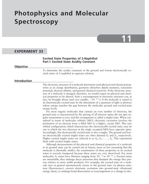
<strong>Photophysics</strong> <strong>and</strong> <strong>Molecular</strong><br />
<strong>Spectroscopy</strong><br />
11<br />
EXPERIMENT 33<br />
Objective<br />
Introduction<br />
Excited State Properties of 2-Naphthol<br />
<strong>Part</strong> I: Excited State Acidity Constant<br />
To determine the acidity constants of the ground <strong>and</strong> lowest electronically excited<br />
states of 2-naphthol in aqueous solution.<br />
The electronic structure of a molecule determines such physical <strong>and</strong> chemical properties<br />
as its charge distribution, geometry (therefore dipole moment), ionization<br />
potential, electron affinity, <strong>and</strong> general chemical reactivity. If the electronic structure<br />
of a molecule is changed, therefore, we would expect its physical <strong>and</strong> chemical<br />
properties to be altered. Such a rearrangement in electronic structure can, in<br />
fact, be brought about (<strong>and</strong> very rapidly, 10 13 s) if the molecule is raised to<br />
an electronically excited state by the absorption of a quantum of light (a photon)<br />
whose energy matches the gap between the molecular ground <strong>and</strong> excited-state<br />
energy levels.<br />
For most organic molecules that contain an even number of electrons, the<br />
ground state is characterized by the pairing of all electron spins; the net spin angular<br />
momentum is zero, <strong>and</strong> this arrangement is called a singlet state. When considered<br />
in terms of molecular orbitals (MO), electornic excitation involves the<br />
promotion of an electron from a filled MO to a higher, vacant MO. This new<br />
orbital configuration, which characterizes the electronically excited state, may be<br />
one in which the two electrons in the singly occupied MOs have opposite spins.<br />
Accordingly, this electronically excited state is also a singlet. The ground <strong>and</strong> lowest<br />
electronically excited singlet states are often denoted S 0 <strong>and</strong> S 1 , respectively.<br />
Higher excited singlet states are referred to as S 2 , S 3 , . . . , S n . This experiment<br />
deals with excited singlet states.<br />
Although measurements of the physical <strong>and</strong> chemical properties of a molecule<br />
in its ground state can be carried out at leisure, more or less (assuming that the<br />
molecule is thermally stable), the examination of these properties in its excited<br />
states is severely hampered because these states are very short-lived. For most<br />
molecules, S 1 states have lifetimes ranging from 10. 6 to 10 11 s. Excited states<br />
are metastable; they undergo decay processes that dissipate the energy they possess<br />
relative to more stable products. For example, the excited state of a molecule<br />
may in general spontaneously return to the ground state via photon emission<br />
(fluorescence), convert electronic excitation into ground-state vibrational<br />
energy (heat), or undergo bond dissociation or rearrangement or a change in elec-
11-2 PART 11 <strong>Photophysics</strong> <strong>and</strong> <strong>Molecular</strong> <strong>Spectroscopy</strong><br />
tron spin multiplicity. Because spontaneous emission from an excited state (that<br />
is, fluorescence) often takes place very rapidly, fluorescence can be used as a probe,<br />
or measurement, of excited-state concentration (for example, fluorescence assay).<br />
In addition, fluorescence studies can provide information about the physical <strong>and</strong><br />
chemical properties of these short-lived singlet states. This field of experimentation<br />
is called photophysics.<br />
In this experiment, you will determine some ground- <strong>and</strong> excited-state properties<br />
of the organic molecule 2-naphthol (ArOH).<br />
OH<br />
2-Naphthol (ArOH)<br />
In aqueous solution, ArOH behaves as a weak acid, forming the hydronium ion<br />
<strong>and</strong> its conjugate base <strong>and</strong> naphthoxy ion ArO .<br />
ArOH H 2 O 7 ArO H 3 O <br />
It is instructive to measure the acidity constant of ArOH in its lowest excited<br />
electronic state, denoted as K a *, <strong>and</strong> to compare this value with that of the ground<br />
state K a . This information indicates how the change in electronic structure alters<br />
the charge density at the oxygen atom. The experimental method is best introduced<br />
in terms of the energy-level diagram shown in Figure 1.<br />
Figure 1. Schematic<br />
diagram of the ground<br />
<strong>and</strong> first excited singlet<br />
state energies of free<br />
naphthol <strong>and</strong> its<br />
conjugate base, the<br />
naphthoxy ion, in<br />
aqueous solution.<br />
S 1<br />
ArO – *<br />
∆H*<br />
K* a<br />
S 1<br />
ArOH*<br />
h ArO –<br />
h ArOH<br />
S 0<br />
∆H<br />
ArO – + H +<br />
K a<br />
S 0<br />
ArOH<br />
The relative energies of the free acid <strong>and</strong> its conjugate base (the naphthoxy<br />
ion) are indicated for both the electronic ground (S 0 ) <strong>and</strong> (lowest) excited (S 1 )<br />
states in aqueous solution. Each anion is elevated with respect to its free acid by<br />
an energy, H <strong>and</strong> H*, respectively. These are the enthalpies of deprotonation.<br />
Both the ground-state acid <strong>and</strong> its conjugate base can be transformed to their respective<br />
excited states via the absorption of photons of energy hv ArOH <strong>and</strong> h ArO .<br />
For simplicity, these absorptive transitions are shown to be equal to the fluorescence<br />
from the excited to the ground states of the acid <strong>and</strong> conjugate base. (The<br />
ground- <strong>and</strong> excited-state vibrational levels involved in the transitions are not<br />
indicated.)
We can express the free energy of deprotonation of ArOH in terms of the enthalpy<br />
<strong>and</strong> entropy of deprotonation <strong>and</strong> the equilibrium (ionization) constants<br />
<strong>and</strong><br />
Experiment 33<br />
G H T S RT ln K a (1)<br />
G* H* T S* RT ln K a * (2)<br />
for the S 0 <strong>and</strong> S 1 states, respectively. If we make the assumption that the entropies<br />
of dissociation of ArOH <strong>and</strong> (ArOH)* are equal, it follows that<br />
<br />
Ka<br />
11-3<br />
K*<br />
H H* RT ln<br />
<br />
a<br />
, (3)<br />
<strong>and</strong> thus from Figure 1, it can be deduced that<br />
H N A h ArO<br />
H* NA h ArOH , (4)<br />
where h is Planck’s constant. Avogadro’s number N A has been included to put each<br />
energy term on a molar basis. Combining equations (4) <strong>and</strong> (3) <strong>and</strong> rearranging,<br />
K*<br />
ln<br />
<br />
a<br />
N A h( ArO<br />
ArOH )<br />
. (5)<br />
Ka RT<br />
Thus knowledge of the energy gap between the ground <strong>and</strong> first excited states<br />
for both the free acid <strong>and</strong> its conjugate base leads to an estimate of K a *, if K a is<br />
known. The analysis presented here, which accounts for the observed thermodynamic<br />
<strong>and</strong> spectroscopic energy differences, was first developed by Th. Förster<br />
(1949, 1950). This approach is thus often referred to as a Förster cycle. Equation<br />
(5) can be recast into a more convenient form:<br />
N<br />
pK* a pK a A hc<br />
[˜ArOH ˜ArO ], (6)<br />
2.303RT<br />
where c, the speed of light, has been incorporated in the expression to express<br />
the transition energies of ArOH <strong>and</strong> ArO into wavenumbers (cm 1 ), a common<br />
spectroscopic energy unit, rather than Hz (s 1 ). The acidity constants are expressed<br />
as pK values. The 2.303 is needed in the denominator because the pK’s<br />
are defined as log 10 K.<br />
The question now is how to obtain the spectroscopic energy difference (˜ArO <br />
˜ArOH ), or ˜, pertinent to the Förster cycle in 2-naphthol. Three approaches can<br />
be considered. The first is to base the measurement on the absorption maxima of<br />
the free acid <strong>and</strong> conjugate base. The second is to use the fluorescence maxima<br />
of the two species, <strong>and</strong> the third is to use what is called the 0-0 energies of ArOH<br />
<strong>and</strong> ArO . The first two methods are somewhat more straightforward. Obtaining<br />
˜ from absorption data has the advantage that the energy difference that is<br />
obtained does not require an instrumental wavelength correction. Although obtaining<br />
˜ from the fluorescence maxima seems simple enough, fluorimeters usually<br />
produce spectra that are distorted by the wavelength response of the monochromator/photomultiplier<br />
combination. Thus, unless these spectra are corrected<br />
for this sensitivity distortion, the recorded fluorescence maxima will depend (al-
11-4 PART 11 <strong>Photophysics</strong> <strong>and</strong> <strong>Molecular</strong> <strong>Spectroscopy</strong><br />
though perhaps subtly) on the particular instrument used <strong>and</strong> thus will not represent<br />
the “true” or absolute spectroscopic properties of the ArOH/ArO system.<br />
The third approach provides the value of ˜ that best represents the energy<br />
difference between S 1 <strong>and</strong> S 0 implied in the Förster cycle, ˜0-0 . Unfortunately<br />
˜0-0 cannot be determined directly in all cases (such as ArOH), but it can be estimated<br />
from an analysis of both the absorption <strong>and</strong> fluorescence spectra. It is<br />
shown schematically in Figure 2 for a single species (ArOH or ArO ).<br />
˜<br />
max (fluor)<br />
˜<br />
max (abs)<br />
Figure 2. Schematic<br />
diagram of the<br />
absorption <strong>and</strong><br />
fluorescence spectra of a<br />
molecule. It is assumed<br />
that these transitions are<br />
between the same two<br />
electronic states, that is,<br />
S 0 i S 1 .<br />
Fluorescence<br />
˜<br />
00<br />
˜<br />
absorption<br />
Mirror image of fluorescence<br />
Safety Precautions<br />
The absorption <strong>and</strong> (preferably instrument-corrected) fluorescence spectra are<br />
both plotted on a common energy axis. Furthermore, the spectra are presented<br />
so that each has the same peak maximum value. The point of intersection of these<br />
spectra can be approimated as the 0-0 energy gap between S 0 <strong>and</strong> S 1 . This approach<br />
does not apply to cases in which the S 0 –S 1 transition is distorted by a<br />
nearby (<strong>and</strong> especially more intensely absorbing) S 0 to S 2 trnsition.<br />
Whichever method is used to determine ˜, it should be used consistently with<br />
both species ArOH <strong>and</strong> ArO .<br />
◆<br />
Always wear safety goggles in the laboratory. Ultraviolet light-absorbing<br />
eye protection is required. Some plastic safety goggles do not completely<br />
absorb ultraviolet radiation.<br />
◆<br />
◆<br />
2-Naphthol is an irritant. If you are to prepare the solutions from solid<br />
material, you must wear gloves; if possible, work in a fume hood.<br />
Be sure you have been instructed to use the proper pipetting techniques<br />
when h<strong>and</strong>ling 2-naphthol solutions. Never pipet using suction by mouth.<br />
Procedure<br />
◆<br />
If you are to obtain fluorescence spectra, be sure that any ozone produced<br />
by the ultraviolet source is vented. Ozone is a noxious, dangerous gas that<br />
has an acrid odor. If you detect this gas, leave the vicinity, inform your<br />
instructor, <strong>and</strong> increase air circulation at once.<br />
In this experiment, you will determine K a from the pH dependence of the absorption<br />
spectrum of aqueous 2-naphthol.<br />
1. Obtain the absorption spectra of two solutions of ArOH (each at<br />
2 10 4 M; the actual concentration must be accurately known). In one
Experiment 33<br />
11-5<br />
solution, the free acid must predominate (low pH), <strong>and</strong> in the other, the<br />
conjugate base must be the major naphthol component (high pH). Use<br />
stock solutions of HCl <strong>and</strong> NaOH (for example, 0.10 M) to create [H]<br />
<strong>and</strong> [OH ] of 0.02 M, respectively. It is important that the ArOH<br />
concentration be the same in each case. Label <strong>and</strong> save these solutions.<br />
Record or display these spectra on a common wavelength axis so that the<br />
spectra overlap.<br />
2. Now obtain absorption spectra of ArOH (also 2 10 4 M) at<br />
intermediate pH values. Adjust pH levels using ammonium chloride buffer<br />
solutions (NH 4 OH/NH 4 Cl), for example, 0.1 M/0.1 M, 0.1/0.2, or 0.2/0.1.<br />
These solutions can be conveniently prepared from 1.00 M stock solutions<br />
of NH 4 OH <strong>and</strong> NH 4 Cl. Obtain at least three spectra <strong>and</strong> scan the entire<br />
wavelength range as in step 1. These spectra will indicate both free acid<br />
<strong>and</strong> conjugate base absorption. If necessary, choose appropriate ratios of<br />
the NH 4 OH <strong>and</strong> NH 4 Cl stock solutions to produce a satisfactory series of<br />
ArOH/ArO spectra. It is essential that the 2-naphthol concentrations be<br />
identical <strong>and</strong> accurately known in each case. Immediately after recording<br />
each spectrum, measure the actual pH of the solution using a properly<br />
calibrated pH meter. Label <strong>and</strong> save these solutions. It is instructive to<br />
display or overlap each spectrum on a common axis. Make sure that the<br />
temperature of the samples is constant (to within 1°C) or otherwise<br />
controlled throughout the experiment. If the bulk ArOH concentration, for<br />
example, [ArOH] [ArO ], is invariant, the spectra, when properly<br />
overlapped, should intersect at a common wavelength called the isosbestic<br />
(equal absorption) point. The presence of an isosbestic point indicates that<br />
there is a closed system (as a function of the variable, pH) consisting of<br />
two species in equilibrium.<br />
3. Using the same solutions in step 1, obtain the fluorescence spectra of<br />
naphthol <strong>and</strong> its conjugate base. If possible, correct the spectra for the<br />
monochromator/photomultiplier response of the fluorimeter.<br />
4. If possible, display the fluorescence spectra of the intermediate pH solutions<br />
on the same wavelength axis so that the spectra overlap. Again, you should<br />
observe a common wavelength where the spectra overlap. This is sometimes<br />
referred to as an isostilbic (equal brightness) point. Likewise, the presence<br />
of an isostilbic point indicates that there are two excited-state species that,<br />
aside from emitting light, interconvert only with each other.<br />
Calculations<br />
Because the bulk naphthol concentrations [ArOH] 0 are identical in each of the<br />
solutions studied, the following material balance applies:<br />
[ArOH] 0 [ArOH] [ArO ]. (7)<br />
Under the condtioins that (a) both the free acid <strong>and</strong> conjugate base absorb at<br />
max ArOH, the wavelength of maximum absorption for ArOH, <strong>and</strong> (b) Beer’s<br />
law holds,<br />
A( max ArOH) ArOH [ArOH] ArO<br />
[ArO ], (8)
11-6 PART 11 <strong>Photophysics</strong> <strong>and</strong> <strong>Molecular</strong> <strong>Spectroscopy</strong><br />
where A is the absorbance (for a 1-cm path length) <strong>and</strong> ArOH <strong>and</strong> ArO<br />
are the<br />
molar absorptivity coefficients of the free acid <strong>and</strong> conjugate base at max (ArOH),<br />
respectively. Combining equations (7) <strong>and</strong> (8) produces<br />
A( max ArOH) { ArOH ArO<br />
}[ArOH] {ArO }[ArOH]0 . (9)<br />
This relation allows [ArOH] to be determined under equilibrium conditions. Once<br />
it is known, the value of [ArO ] at the same pH can be obtained from equation<br />
(7). Because the acidity constant is<br />
[H<br />
K a 3 O ][ArO ]<br />
<br />
(10)<br />
[ArOH]<br />
(assuming that the activity coefficient ratio is unity in these dilute solutions), you<br />
can obtain the pK a value for ArOH from a linear regression of pH vs.<br />
log([ArO ]/[ArOH]):<br />
[ArO<br />
pH pK a log ]<br />
. (11)<br />
[ArOH]<br />
You can obtain the values of [ArOH] <strong>and</strong> [ArO ] for each solution from equations<br />
(9) <strong>and</strong> (7), respectively. Report the st<strong>and</strong>ard deviation in pK a . Compare<br />
your results with literature values.<br />
Calculate pK a * for (ArOH)* from equation (6) using the pK a value you obtained<br />
<strong>and</strong> whatever method(s) you choose to determine (˜ArOH ˜ArO<br />
). Compare<br />
these values <strong>and</strong> perform an error analysis. Discuss the errors that the primary<br />
measurements have on the derived value of pK a *.<br />
Other molecules that you can study using this procedure are 2-naphthoic acid,<br />
acridine, <strong>and</strong> quinoline. Their solubilities in water are limited but sufficient to allow<br />
you to prepare the dilute solutions needed for the experiments.<br />
O<br />
C<br />
OH<br />
2-Naphthoic acid<br />
N<br />
Acridine<br />
N<br />
Quinoline<br />
Questions <strong>and</strong> Further Thoughts<br />
1. In comparing the values of K a <strong>and</strong> K*, a what can you deduce about the change in electron<br />
density at the O atom in 2-naphthol in the electronically excited state relative to the<br />
ground state If you have access to a molecular orbital program, such as HyperChem,<br />
MOPAC, or Gaussian, perform a suitable MO calculation on the ground <strong>and</strong> first excited<br />
singlet states of 2-naphthol. The AM1 Hamiltonian is appropriate, <strong>and</strong> a configuration<br />
interaction calculation involving at least the highest-filled <strong>and</strong> lowest-unfilled<br />
molecular orbitals is required for the excited-state property. These calculations will provide<br />
the atomic electronic charges.<br />
2. If pK* a pK a (the excited-state species is a stronger acid), can you comment on the relative<br />
(absolute) magnitudes of the enthalpies of deprotonation See Figure 1.
Experiment 33<br />
11-7<br />
Further Readings<br />
3. On what basis can we justify the assumption that the entropies of deprotonation of<br />
the ground- <strong>and</strong> excited-state 2-naphthol molecules are equal [see equations (1)–(3)]. Can<br />
you think of another possibility in which this assumption is a poor one<br />
4. Ohter molecules that can be studied using this technique are 2-naphthoic acid, acridine,<br />
<strong>and</strong> quinoline (see the last paragraph in the Calculations section). Indicate the protolytic<br />
reactions for these molecules, i.e., write the aqueous acid-base reactions.<br />
5. Can you predict before doing an experiment whether the excited state of a molecule<br />
is a stronger or weaker acid than its respective ground state What information would<br />
you need to perform such an assessment<br />
General<br />
P. Atkins <strong>and</strong> J. de Paula, Physical Chemistry, 8th ed., p. , W. H. <strong>Freeman</strong> (New York),<br />
2006.<br />
I. N. Levine, Physical Chemistry, 5th ed., pp. 777–780, McGraw-Hill (New York), 2002.<br />
R. J. Silbey, R. A. Alberty, <strong>and</strong> M. G. Bawendi, Physical Chemistry, 4th ed., pp. 519–522,<br />
Wiley (Hoboken, NJ), 2005.<br />
Förster Cycle <strong>and</strong> Excited-State Acidity<br />
Th. Förster, Naturwiss., 36:186 (1949).<br />
Th. Förster, Z. Electrochem., 54:531 (1950).<br />
C. Parker, Photoluminescence of Solutions, pp. 328–341, Elsevier (Amsterdam), 1968.<br />
J. Van Stam <strong>and</strong> J. E. Loefroth, J. Chem. Educ., 63:181 (1986).<br />
A. Weller, in G. Porter, ed., Progress in Reaction Kinetics, vol. 1, pp. 189–214, Pergamon<br />
(New York), 1961.<br />
Fluorescence <strong>and</strong> <strong>Photophysics</strong><br />
J. B. Birks, <strong>Photophysics</strong> of Aromatic Molecules, Wiley-Interscience (London), 1970.<br />
J. R. Lakowicz, Principles of Fluorescence <strong>Spectroscopy</strong>, Plenum Press (New York), 1983.<br />
N. J. Turro, Modern <strong>Molecular</strong> Photochemistry, Benjamin/Cummings (Menlo Park, CA),<br />
1978.
EXPERIMENT 34<br />
Objective<br />
Introduction<br />
Excited-State Properties of 2-Naphthol<br />
<strong>Part</strong> II: Deprotonation <strong>and</strong> Protonation Rate Constants<br />
To determine the deprotonation <strong>and</strong> protonation rate constants of 2-naphthol in<br />
its lowest excited singlet state in aqueous solution.<br />
In the previous experiment, we determined acidity constants for aqueous<br />
2-naphthol (ArOH) for both the ground <strong>and</strong> lowest excited (singlet) states. These<br />
constants pertain to the equilibrium<br />
k d<br />
ArOH H2 O 0ˆ ˆ9 ArO H 3 O , (1)<br />
k p<br />
where the rate constants for the forward (deprotonation) <strong>and</strong> reverse (protonation)<br />
reactions are indicated as k p <strong>and</strong> k d , respectively. A similar equilibrium can<br />
be written for the electronically excited-state species, which is produced via photon<br />
absorption:<br />
k d <br />
ArOH* H 2 O 0ˆ ˆ9 ArO * H 3 O , (2)<br />
k p <br />
in which the values of the forward- <strong>and</strong> reverse-rate constants may be different<br />
from those in the ground state because of differences in the properties of the<br />
2-naphthol in these two states (for example, different K a values).<br />
We can express the ratio of the concentrations of free acid <strong>and</strong> the conjugate<br />
base as a function of the pH:<br />
[ArOH]<br />
[ArO ]<br />
log<br />
pK a pH, (3a)<br />
where we use molar concentrations to approximate activities. An analogous<br />
equation,<br />
[ArOH*]<br />
[ArO *]<br />
log<br />
pK a* pH (3b)<br />
applies to excited state species. Equations (3a) <strong>and</strong> (3b) show that if the pH of<br />
the solution is less than pK a of 2-naphthol (in either electronic state), the free acid<br />
form will predominate over that of conjugate base: [ArOH] [ArO ]. Likewise,<br />
if pH pK a , then [ArO ] [ArOH].<br />
Suppose that by using a suitable buffer, the pH of the medium is established<br />
to be less than pK a but greater than pK a *. The ground state of the system will<br />
then consist primarily of ArOH. Electronic excitation via light absorption will instantaneously<br />
(10 13 s) transform ArOH into ArOH*. We may assume that in<br />
this experiment, the buffer holds the pH of the medium constant during <strong>and</strong> after<br />
electronic excitation. This is a valid assumption because the number of photons<br />
absorbed per unit volume is much less than the ground-state concentration
Experiment 34<br />
11-9<br />
of ArOH. Thus [ArOH*] [ArOH]; moreover, ArOH* will spontaneously dissociate<br />
to form ArO * in order to establish new equilibrium conditions. Under<br />
these circumstances, [ArO *] must be greater than [ArOH*] because pH pK a *<br />
[see equation (3a)]. In fact, most of the fluorescence observed from ArO * takes<br />
place from species that were formed via ArOH* deprotonation after elecronic excitation.<br />
As excited-state equilibrium is approached, the ArOH* concentration<br />
decreases while that of ArO * increases. The strategy of this experiment in determining<br />
k d <strong>and</strong> k p is to measure the dependence of [ArOH*] on the pH of the<br />
solution. [ArOH*] is monitored through its fluorescence intensity I f , assuming<br />
that it is proportional to [ArOH*] (see the next section). The pH is established<br />
(<strong>and</strong> varied) using an ammonium acetate buffer.<br />
Kinetic Analysis<br />
Because in this experiment pH pK a , we consider only light absorption by the<br />
protonated form ArOH:<br />
ArOH h abs ArOH*.<br />
(absorption)<br />
The ArOH* thus produced is, like any excited state, metastable, <strong>and</strong> when it relaxes<br />
(dissipates the excitation energy) it can undergo a number of different decay<br />
processes, such as<br />
k r<br />
1. ArOH* l ArOH h fluor (fluorescence) rate k r [ArOH*].<br />
k nr<br />
2. ArOH* l ArOH heat (nonradiative decay) rate k nr [ArOH*]<br />
k d<br />
3. ArOH* l ArO * H (aq) (deprotonation) rate k d [ArOH*]<br />
k Ac <br />
4. ArOH* Ac l ArO * HAc (deprotonation via Ac ) rate k Ac<br />
[ArOH*][Ac ]<br />
In addition to radiative (fluorescence) decay (1) <strong>and</strong> nonradiative relaxation<br />
(2), ArOH* can undergo “unassisted” (3) <strong>and</strong> “acetate-assisted” (4) deprotonation.<br />
This distinction is significant because the rate of deprotonation will be enhanced<br />
in the presence of the acetate ion in the bimolecular step indicated in<br />
process 4. Undoubtedly, solvent plays a role in the unassisted deprotonation (3),<br />
but this step can be considered pseudo first order in ArOH* because the concentration<br />
of “solvent” is so much larger than [ArOH*]. The reverse steps of the<br />
deprotonation processes, which are bimolecular <strong>and</strong> proportional to [H 3 O ] <strong>and</strong><br />
[HAc] (see steps 3 <strong>and</strong> 4, respectively), are ignored because under these experimental<br />
conditions, [H 3 O ] <strong>and</strong> [HAc] are very small.<br />
If the pH of the solution is much lower than pK a * (for example, in the presence<br />
of sulfuric acid), deprotonation by either process is suppressed <strong>and</strong> fluorescence<br />
from ArOH* predominates. In this case, the fluorescence intensity I f 0 , which<br />
is proportional to the ratio of the rate of radiative decay to the total ArOH* decay<br />
rate, can be expressed<br />
I 0 Ck<br />
f r [ArOH*]<br />
, (4)<br />
k r [ArOH*] k nr [ArOH*]
11-10 PART 11 <strong>Photophysics</strong> <strong>and</strong> <strong>Molecular</strong> <strong>Spectroscopy</strong><br />
or, canceling [ArOH*],<br />
I 0 Ck<br />
f , r<br />
, (5)<br />
kr k nr<br />
where C is an instrumental constant.<br />
In contrast, when pH pK a * (but less than pK a ) under NH 4 Ac buffer conditions,<br />
the deprotonation steps become kinetically important, <strong>and</strong> thus the denominator<br />
of equation (4) will contain the aditional terms k d [ArOH*] <strong>and</strong><br />
k Ac<br />
[ArOH*][Ac ]. Therefore, the ArOH* fluorescence intensity, now denoted<br />
as I f , become [see equation (5)]<br />
Ck<br />
I f <br />
r<br />
. (6)<br />
k r k nr k d k Ac[Ac ]<br />
The deprotonation of ArOH* causes a diminution in its fluorescence intensity;<br />
thus I f I f 0 . Assuming that [ArOH*] is identical in all the solutions studied, the<br />
ratio of ArOH* fluorescence intensity in a solution containing sulfuric acid (low<br />
pH) to that containing ammonium acetate buffer (higher pH) is obtained by dividing<br />
equation (5) by (6):<br />
0<br />
I k<br />
r k nr k d k Ac<br />
[Ac f ]<br />
.<br />
If<br />
kr k nr<br />
(7)<br />
0<br />
I f<br />
<br />
1 k<br />
d<br />
<br />
If kr k nr kr k nr<br />
(8)<br />
We can rearrange equation (7) to a more convenient form,<br />
or<br />
k Ac<br />
[Ac ]<br />
0<br />
I f<br />
<br />
If<br />
<br />
1 0k d 0 k Ac<br />
[Ac ],<br />
where 0 1/(k r k nr ) <strong>and</strong> is the “lifetime” of ArOH* in the absence of significant<br />
deprotonation. A plot of ( I 0 f /I f 1) versus [Ac ] should be linear with slope<br />
0 k Ac<br />
<strong>and</strong> intercept 0 k d . To determine k d , one must obtain 0 from a separate<br />
experiment.<br />
The information provided by this type of study, which involves timeindependent,<br />
or steady-state, measurements could also be obtained directly using<br />
a transient, or kinetic, approach by monitoring the fluorescence decay of ArOH*.<br />
After photoexcitation by a very short pulse of light (10 9 s), the ArOH* fluorescence<br />
intensity follows the first-order decay law<br />
I f (t) [ArOH*] 0 exp{(k r k nr k d k Ac<br />
[Ac ])t}, (9)<br />
where [ArOH*] 0 is the concentration of photoexcited ArOH produced immediately<br />
after excitation (at t 0) <strong>and</strong> t is the time after excitation. Note again that<br />
equation (9) represents the proportionality between fluorescence intensity <strong>and</strong> excited-state<br />
concentration. The coefficient of t in equation (9) is the reciprocal of<br />
the fluorescence lifetime of ArOH*, (1/ Ac<br />
), in the presence of the NH4 Ac buffer.
Experiment 34 11-11<br />
The information provided by the steady-state Stern-Volmer-like plot—equation<br />
(8)—could be directly obtained from a plot of 1/ Ac<br />
versus [Ac ]. These experiments<br />
can be carried out using a nanosecond (10 9 s) fluorescence decay<br />
spectrometer.<br />
In this experiment, you will obtain k d using steady-state approach previously<br />
described. You can obtain the value of 0 from the provided data for the time dependence<br />
of ArOH* fluorescence intensity. This information comes from a fluorescence<br />
decay experiment (see the Appendix to this experiment). We emphasize<br />
again that in deriving equations (4) to (8), it is assumed that throughout the series<br />
of fluorescence intensity measurements, first in sulfuric acid <strong>and</strong> then in different<br />
NH 4 Ac buffer solutions, the concentration of ArOH* is invariant. This<br />
condition requires that the amount of light absorbed by ArOH per unit time be<br />
constant; thus, not only must the formal concentration of 2-naphthol be identical<br />
in each of the samples but also the intensity of the excitation source must not<br />
fluctuate. Satisfying these conditions is crucial for the success of the experiment.<br />
Once you obtain a value of k d from the analysis of the data as discussed, you<br />
can determine the value of k p (the protonation rate constant for the excited state<br />
naphthoxy ion) from K* a because<br />
k<br />
K* a d<br />
(10)<br />
kp<br />
for this set of elementary reactions.<br />
Safety Precautions<br />
◆<br />
◆<br />
◆<br />
◆<br />
Always wear safety goggles; these glasses should block ultraviolet light.<br />
Ordinary plastic safety goggles or glasses may not be effective in absorbing<br />
all the ultraviolet radiation. Check with your instructor.<br />
2-Naphthol is an irritant. If you are to prepare the solutions from solid<br />
material, you must wear gloves; if possible, work in a fume hood.<br />
Be sure you have been instructed to use proper pipetting techniques when<br />
h<strong>and</strong>ling 2-naphthol. Never pipet by mouth.<br />
When using the fluorimeter, be sure that any ozone produced by the<br />
ultraviolet source is vented. Ozone is an irritating, dangerous gas that has a<br />
sharp, pungent odor. If you notice this kind of odor during the experiment,<br />
inform your instructor at once. The laboratory must be immediately<br />
ventilated <strong>and</strong>, if necessary, evacuated.<br />
Procedure Using Scanning Fluorimeter<br />
1. Prepare a series of aqueous solutions in 25-mL volumetric flasks, each<br />
having the same ArOH concentration (about 4.0 10 4 M). One of them<br />
will be 0.1 M in H 2 SO 4 (for I f 0 ), another 0.1 M in NaOH (in order<br />
to observe predominantly ArO * fluorescence). The remainder of the<br />
solutions will have varying NH 4 Ac concentrations between 0.01 M <strong>and</strong><br />
0.10 M. Study at least five NH 4 Ac-containing ArOH solutions in this<br />
range. Stock solutions of H 2 SO 4 , NaOH, ArOH, <strong>and</strong> NH 4 Ac will be<br />
provided. Label each solution <strong>and</strong> record the ambient temperature.<br />
2. You will be shown how to operate the fluorimeter. Using an excitation<br />
wavelength of 320 nm, obtain the fluorescence spectra of the ArOH
11-12 PART 11 <strong>Photophysics</strong> <strong>and</strong> <strong>Molecular</strong> <strong>Spectroscopy</strong><br />
solutions starting with the solution containing H 2 SO 4 . Next, obtain the<br />
fluorescence spectrum of the NaOH-containing solution. Then proceed with<br />
the NH 4 Ac-containing solutions in order of increasing NH 4 Ac<br />
concentraion. It is recommended that you display these spectra on a<br />
common wavelength scale. If the excitation source remains steady <strong>and</strong> the<br />
solutions have the same bulk ArOH concentrations, a distinct isostilbic<br />
(equal brightness) point should be produced. This is the common<br />
wavelength point of all the ArOH fluorescence spectra. See Experiment 34<br />
for a further discussion of the isostilbic point.<br />
Data Analysis<br />
3. If a fixed-wavelength fluorimeter is used or if time permits, perform a<br />
second determination of data at the emission wavelength of the fluorimeter<br />
corresponding to the maximum for the protonated ArOH* (360 nm).<br />
First, place the H 2 SO 4 -containing sample in the cavity <strong>and</strong> establish the<br />
“maximum” intensity setting on the chart paper by moving the pen close to<br />
its full displacement (or just read <strong>and</strong> record the signal strength). Carefully<br />
<strong>and</strong> systematically obtain values of the fluorescence intensity of the<br />
buffered solutions in order of increasing NH 4 Ac concentrations. If there is<br />
any doubt about the constancy of the instrument, remeasure I f 0 <strong>and</strong><br />
compare it with the original value. If the agreement is unsatisfactory, you<br />
will have to repeat the series of measurements.<br />
1. Using the time-dependent fluorescence intensity data provided in the<br />
Appendix for ArOH in 0.10 M H 2 SO 4 , determine 0 . The fluorescence<br />
quantum efficiency of ArOH under these conditions has been determined<br />
to be 0.18; this quantity is equal to k r 0 . Report values of both k r <strong>and</strong> k nr<br />
for ArOH.<br />
2. Tabulate I f 0 <strong>and</strong> the I f <strong>and</strong> corresponding [Ac ] values for the samples, <strong>and</strong><br />
construct a Stern-Volmer-like plot indicated by equation (8). Determine<br />
values of k d <strong>and</strong> k Ac<br />
<strong>and</strong> their st<strong>and</strong>ard deviations using linear regression.<br />
Consider the error in 0 [obtained in step (1)] in your error analysis of the<br />
rate constants.<br />
3. Determine k p from your previously obtained value of K a * [see equation (10)].<br />
4. Tabulate all the rate constants determined <strong>and</strong> include estimates of their<br />
respective uncertainties.<br />
5. Using the Stokes-Einstein-Smolouchowski (SES) equation for a diffusioncontrolled<br />
rate constant (see Experiment 22), calculate k diff :<br />
8000RT<br />
k diff (dm 3 mol 1 s 1 ),<br />
3<br />
where is the solvent viscosity. The indicated units for k diff are obtained if<br />
R <strong>and</strong> are in SI units, that is, 8.314 J K 1 , <strong>and</strong> in N m 2 s, respectively<br />
(1 cP 10 3 N m 2 s). Compare your values of the second-order rate<br />
constants k d <strong>and</strong> k Ac<br />
with kdiff . You can use the viscosity of water at the<br />
appropriate temperature for this comparison. The SES equation applies to<br />
the reaction between two neutral species (or a neutral <strong>and</strong> a charged<br />
reaction pair). For anion–cation pairs (each of single charge), the rate<br />
constant is about an order of magnitude larger than k diff .
Experiment 34<br />
11-13<br />
Questions <strong>and</strong> Further Thoughts<br />
Further Readings<br />
1. The pH of the aqueous medium is assumed to be unchanged as a result of electronic<br />
excitation of 2-naphthol. Why is this justified<br />
2. Can you predict how the value of the deprotonation rate constant of ArOD* (ArOD)<br />
would differ from that of ArOH* (ArOH) What would you need to know to answer<br />
this question<br />
3. Can you suggest an experiment in which the deprotonation rate constant of ArOH<br />
(ground state) could be determined<br />
4. Ozone is sometimes produced by ultraviolet light sources. What is the mechanism by<br />
which ozone is produced Can you suggest a way in which the ozone production by a<br />
given ultraviolet source can be eliminated<br />
5. As the source of acetate ion you used ammonium acetate. Why is this compound chosen<br />
What would be the advantage or disadvantage of using sodium acetate<br />
2-Naphthol Protolysis<br />
R. Boyer, G. Deckey, C. Marzzacco, M. Mulvaney, C. Schwab, <strong>and</strong> A. M. Halpern, J.<br />
Chem. Educ., 62:630, 1985.<br />
J. Van Stam <strong>and</strong> J. E. Loefroth, J. Chem. Educ., 63:181 (1986).<br />
Appendix<br />
Fluorescence <strong>and</strong> <strong>Photophysics</strong><br />
J. R. Lakowicz, Principles of Fluorescence <strong>Spectroscopy</strong>, Plenum Press (New York), 1983.<br />
N. J. Turro, Modern <strong>Molecular</strong> Photochemistry, Benjamin/Cummings (Menlo Park, CA),<br />
1978.<br />
Fluorescence Decay Data for 2-Naphthol<br />
in 0.10 M H 2 SO 4 at 25°C<br />
Time (ns)<br />
Intensity*<br />
0.00 21753<br />
1.00 18907<br />
2.00 16380<br />
3.00 14171<br />
4.00 12432<br />
5.00 10757<br />
6.00 9288<br />
7.00 8138<br />
8.00 7083<br />
9.00 6014<br />
10.00 5350<br />
*Photons emitted per unit time.
EXPERIMENT 35<br />
Objective<br />
Introduction<br />
Enthalpy <strong>and</strong> Entropy of Excimer Formation<br />
To determine the enthalpy <strong>and</strong> entropy of formation of the dimer between ground<br />
state <strong>and</strong> electronically excited pyrene molecules in solution.<br />
We know that the physical <strong>and</strong> chemical properties of a molecule are dictated by<br />
the nature of its electronic structure. It is not surprising, therefore, that such properties<br />
as acidity, dipole moment, <strong>and</strong> chemical reactivity may change considerably<br />
on electronic excitation, in which there is a very rapid change in the characteristics<br />
of a species’ electronic wavefunction. In this experiment, you will<br />
investigate the pairwise interaction between pyrene molecules. We are interested<br />
in determining how the interaction potential between two ground-state molecules<br />
differs from that between an electronically excited molecule <strong>and</strong> its ground-state<br />
counterpart.<br />
Consider, then, the approach of two pyrene molecules along an axis perpendicular<br />
to their molecular planes. If both molecules are in the ground electronic<br />
state, there will be a very weak van der Waals attraction at moderate distances.<br />
As they become closer, of course, significant intermolecular repulsion occurs. If,<br />
however, one of the molecules is in its electronically excited state (as a result of<br />
light absorption) <strong>and</strong> is allowed to approach a ground-state species with the appropriate<br />
orientation, a stable dinner will form. This dimer, whose structure is<br />
proposed to have a “s<strong>and</strong>wich” configuration, is formed reversibly; that is, it can<br />
thermally dissociate back into an electronically excited pyrene molecule (excited<br />
monomer) <strong>and</strong> a ground-state species. 1 This unusual dimeric species is stable as<br />
long as it possesses electronic excitation but dissociates as soon as this electronic<br />
excitation is dissipated <strong>and</strong> the system returns to the ground state. Such a species<br />
is called an excimer (from excited dimer).<br />
Pyrene<br />
Pyrene crystal dimer<br />
A bound state that arises from the interaction between two dissimilar species,<br />
one in its electronically excited state, is sometimes called an exciplex (excited complex).<br />
Like an excimer, an exciplex is dissociative in the electronic ground state.<br />
Because the excimer forms only when an electronically excited molecule <strong>and</strong> a
Experiment 35<br />
11-15<br />
ground state molecule come into specific <strong>and</strong> close contact with each other, excimer<br />
fluorescence is often used as a probe of molecular interactions. For example,<br />
pyrene end-capped polymers are used to study the conformational structure<br />
<strong>and</strong> dynamics of alkane chains. Excimer (or exciplex) emission is also used as a<br />
probe of the intercalation or binding of aromatic molecules into the crevices of<br />
certain macromolecules.<br />
Figure 1 illustrates the potential energy diagram for electronic transitions <strong>and</strong><br />
excimer formation. At large intermolecular separation (which pertains to low concentration),<br />
electronic transitions involving the excited monomer (absorption <strong>and</strong><br />
fluorescence) are shown. The involvement of molecule vibrations in these transitions<br />
is also indicated. Although the monomer absorption <strong>and</strong> fluorescence spectra<br />
show vibrational structure (usually involving a skeletal mode), excimer emission<br />
is structureless. This is characteristic of electronic transitions (absorption or<br />
emission) between bound <strong>and</strong> unbound states.<br />
B<br />
Figure 1. Potential<br />
energy of two pyrene<br />
molecules as a function<br />
of intermolecular<br />
separation. The<br />
coordinate r describes<br />
the approach of the<br />
molecules having the<br />
equilibrium orientation<br />
of the excimer. The<br />
right-h<strong>and</strong> transitions<br />
represent the isolated<br />
monomer (M).<br />
V(r)<br />
h D M00<br />
h M<br />
R<br />
r<br />
The maximum in the excimer emission spectrum corresponds to transitions<br />
between the minimum of the excimer potential well (which exists at the equilibrium<br />
separation between the excimer components) <strong>and</strong> the unbound, ground-state<br />
dimer having the same intermolecular separation as the excimer. Hence, excimer<br />
formation involves the creation of a bound species subsequent to photon absorption.<br />
Conceptually, this is the reverse of photodissociation, in which light absorption<br />
results in bond breakage. Moreover, photon emission in the excimer (fluorescence)<br />
brings about molecular dissociation, since the repulsive ground-state<br />
pair rapidly dissociates.<br />
The potential energy diagram in Figure 1 can also be used to compare the<br />
emission energies of monomer <strong>and</strong> excimer in terms of the excimer binding energy<br />
B <strong>and</strong> the ground-state repulsion energy R. Thus,<br />
h M h D B R, (1)<br />
where h M represents the monomer fluorescence energy (called the 0-0 energy because<br />
the transition takes place between excited- <strong>and</strong> ground-state monomers pos-
11-16 PART 11 <strong>Photophysics</strong> <strong>and</strong> <strong>Molecular</strong> <strong>Spectroscopy</strong><br />
sessing zero quanta of vibrational energy), <strong>and</strong> h D is the energy of the excimer<br />
fluorescence maximum. The binding energy of the excimer is just the negative of<br />
its enthalpy of formation, that is, B H (the system is studied at constant<br />
pressure).<br />
Kinetic Scheme<br />
Excimer formation (called photoassociation) <strong>and</strong> reversible dissociation can be<br />
represented by the following set of elementary processes, or mechanism.<br />
Process Equation Rate Constant<br />
Electronic excitation M h abs M* (rate I abs )<br />
Photoassociation M* M D* k DM<br />
Excimer dissociation D* M M* k MD<br />
Excited monomer decay M* M h M k fM<br />
M* M k iM<br />
Excimer decay D* (M 2 )h D k fD<br />
D* 2M k iD<br />
M<br />
hv abs<br />
k fM<br />
M k DM<br />
M*<br />
D*<br />
kiM k MD M k iD k fD<br />
M hv M M 2M 2M hv D<br />
In this scheme, I abs is the number of moles of photons (einsteins) absorbed by groundstate<br />
monomer per cubic decimeter per second. For convenience, k M <strong>and</strong> k D are defined<br />
as the total intrinsic (intramolecular) decay rate constants of monomer <strong>and</strong> excimer,<br />
respectively, independent of photoassociation or dissociation:<br />
k M k fM k iM <strong>and</strong> k D k fD k iD . (2)<br />
k DM is the second-order rate constant for excimer formation from M <strong>and</strong> M*<br />
(DM denotes “dimer from monomer”), <strong>and</strong> k MD refers to the first-order rate constant<br />
for the dissociation of the excimer into M* <strong>and</strong> M (MD denotes “monomer<br />
from dimer”). The formation rate of excited monomer (in mol dm 3 s 1 ) is<br />
d[M*]<br />
dt<br />
I abs (k M k DM [M])[M*] k MD [D*], (3)<br />
while that for the excimer is<br />
d[D*]<br />
dt<br />
k DM [M][M*] (k D k MD )[D*]. (4)<br />
Note that k DM [M] is the pseudo first-order rate of formation of excimer from excited-<br />
<strong>and</strong> ground-state monomers. Also, it is implied that [M*] [M]; that is,
Experiment 35 11-17<br />
a very small fraction of monomer is electronically excited. In experiments using<br />
conventional light sources (arc lamps, not focused lasers) this is indeed the case.<br />
Under conditions of steady-state illumination, the rates in both equations (3)<br />
<strong>and</strong> (4) are equal to zero (photostationary conditions). The ratio of [D*] to [M*]<br />
can be thus obtained:<br />
[D*] kD<br />
<br />
M[ M]<br />
. (5)<br />
[M*] k D kMD<br />
It st<strong>and</strong>s to reason that since the objective of this experiment is the determination<br />
of thermodynamic quantities, we must determine the temperature dependence<br />
of the excimer formation equilibrium constant. Therefore, the first thing<br />
we need to do is to obtain the equilibrium concentrations of M, M*, <strong>and</strong> D*.<br />
First, we will assume that the equilibrium ground-state concentration [M] is equal<br />
to the bulk pyrene concentration, consistent with the inequality [M*] [M] discussed.<br />
The second crucial (<strong>and</strong> fundamental) assumption is that the fluor (or fluorescent<br />
species) concentration ([M*] or [D*]) is proportional to its respective<br />
fluorescence intensity. This is a basic tenet of spectrofluorimetry <strong>and</strong> is perhaps<br />
analogous to Beer’s law in absorption spectrophotometry.<br />
This experiment is based on the possibility of obtaining the ratio of excimer<br />
to excited monomer concentrations from the measured fluorescence intensities,<br />
each measured at the appropriate wavelength. Both the fluor concentrations are<br />
assumed to be proportional to the respective integrated fluorescence intensities<br />
(areas under the monomer <strong>and</strong> excimer fluorescence spectra),<br />
I fM k fM [M*] <strong>and</strong> I fD k FD [D*], (6)<br />
where the proportionality constants are the radiative rate constants. The dimensions<br />
of I f are einsteins dm 3 s 1 (an einstein is 1 mol of photons). Combining<br />
equations (5) <strong>and</strong> (6),<br />
I k<br />
fD k DM [M]<br />
fD<br />
. (7)<br />
IfM kfM (k D k MD )<br />
Equation (7) is central to the application of photostationary techniques to the<br />
study of photoassociation. (The distinction between the integrated <strong>and</strong> “instantaneous”<br />
fluorescence intensities will be discussed later.)<br />
Because we seek thermodynamic data, we examine the temperature dependence<br />
of equation (7). First, we make the general observation that both the formation<br />
<strong>and</strong> dissociation rate constants are temperature-dependent <strong>and</strong> can be expressed<br />
in Arrhenius form:<br />
E<br />
k DM A DM exp R<br />
DM<br />
T<br />
<strong>and</strong> k MD A MD exp E<br />
MD<br />
R <br />
T ,<br />
(8)<br />
where the A’s <strong>and</strong> E’s are the preexponential factors <strong>and</strong> activation energies, respectively.<br />
Because intermolecular excimer formation is restricted only by molecular<br />
transport, or diffusion, the activation energy E DM is related to the activation to<br />
viscous flow of the solvent medium. E MD , however, reflects the intrinsic strength of<br />
the “excimer bond” as well as the energetics of molecular diffusion. This is because<br />
E MD represents the activation energy for the dissociation ofthe bound excimer<br />
into separated <strong>and</strong> individually solvated excited- <strong>and</strong> ground-state constituents.
11-18 PART 11 <strong>Photophysics</strong> <strong>and</strong> <strong>Molecular</strong> <strong>Spectroscopy</strong><br />
If we assume that the temperature dependence of k MD , the rate constant for<br />
thermally activated excimer dissociation, is much larger than that for k D , the intrinsic<br />
decay rate of excimer (indeed, for many systems, k D is nearly temperatureindependent),<br />
k MD k D in the limit of high temperature. Applying this result<br />
to equation (7),<br />
I fD<br />
<br />
IfM<br />
k<br />
fD k DM [M]<br />
(high temperature). (9)<br />
kfM k MD<br />
If we furthermore make the general assumption (which has been confirmed by<br />
measurements of several monomer/excimer systems) that both radiative rate constants<br />
(k fM <strong>and</strong> k fD ) are temperature-independent, an Arrhenius plot of I fD /I fM<br />
yields, in the limit of high temperature, a slope<br />
I<br />
d ln <br />
f D<br />
I f M (E<br />
DM E MD )<br />
(high temperature). (10)<br />
1<br />
d R<br />
<br />
T<br />
See equations (7) <strong>and</strong> (8). Because E MD E DM , the desired binding energy (the<br />
negative of the enthalpy of formation) of the excimer can be determined as the<br />
slope of such a plot.<br />
At low temperatures, where excimer dissociation is slow compared with its intrinsic<br />
decay rate (k MD k D ), we can write equation (7) as<br />
I fD k fD k DM [M]<br />
(low temperature). (11)<br />
IfM<br />
kf Mk D<br />
An Arrhenius plot of the left-h<strong>and</strong> side of (7) will have a slope approaching<br />
I<br />
d ln <br />
f D<br />
I f M<br />
<br />
1<br />
d <br />
T<br />
E DM<br />
(low temperature). (12)<br />
R<br />
E DM has been found to be closely related to the activation energy associated with<br />
molecular diffusion (hence bulk viscous flow) in the solvent medium. This is one<br />
of the reasons that excimer formation is interpreted as a diffusion-controlled<br />
process.<br />
An Arrhenius plot of equation (7) illustrates the behavior of the monomer <strong>and</strong><br />
excimer fluorescence spectra over a wide temperature range (Figure 2). At low<br />
temperature, the ratio of excimer to monomer emission is small because excimer<br />
formation is impeded by the high viscosity of the solvent; indeed, in a glass or<br />
rigid medium, excimer formation does not take place because of the inability of<br />
excited-monomer <strong>and</strong> ground-state species to diffuse. (It is possible, however, that<br />
weak van der Waals dimers may be stable at low temperatures <strong>and</strong> that emission<br />
from these directly photoexcited dimers may be observed. Strictly speaking, this<br />
is not excimer emission.) At very high temperature, excimer emission is also suppressed<br />
because of the high dissociation rate of the excimer. Thus there is an intermediate<br />
temperature at which there is a maximum excimer emission intensity
Figure 2. Arrhenius plot<br />
of the ratio of excimer<br />
to monomer<br />
fluorescence intensities.<br />
The low-temperature<br />
regime (right) reflects<br />
the activation energy of<br />
excimer formation,<br />
whereas the hightemperature<br />
regime<br />
(left) indicates the<br />
“equilibrium” enthalpy<br />
of excimer formation.<br />
In<br />
l fD<br />
l fM<br />
Experiment 35<br />
k k fM I fD<br />
K eq DM<br />
.<br />
kMD kfD I fM [M]<br />
(13)<br />
11-19<br />
High T<br />
1/T<br />
Low T<br />
k DM [M] k M <strong>and</strong> k MD k D ,<br />
relative to the excited monomer. This temperature depends not only on the nature<br />
of the excimer system (its binding energy <strong>and</strong> entropy of formation) but also<br />
on the solvent characteristics, such as its viscosity <strong>and</strong> activation to viscous flow.<br />
Another very important condition, which is pertinent to the high-temperature<br />
limit <strong>and</strong> is crucial to this experiment, concerns the fact that if interconversion<br />
between photoexcited monomer <strong>and</strong> excimer is rapid relative to the intrinsic decay<br />
rates of M* <strong>and</strong> D*, these species are in dynamic equilibrium. Thus with<br />
K eq [D*] eq /[M*] eq [M] eq , <strong>and</strong> we can express the true equilibrium constant (we<br />
assume unit activity coefficients) for photoassociation as the ratio of the formation<br />
<strong>and</strong> dissociation rate constants. Using this result <strong>and</strong> rearranging equation<br />
(9),<br />
The high-temperature or dynamic equilibrium regime can be depicted by an<br />
analogy to two leaky containers connected to each other by two tubes, each containing<br />
a pump (Figure 3). The containers are filled with a liquid. If the leak rate<br />
A<br />
B<br />
A<br />
A<br />
B<br />
B<br />
Figure 3. Hydrodynamic<br />
model of reversible<br />
reactions between two<br />
metastable<br />
(electronically excited)<br />
species.
11-20 PART 11 <strong>Photophysics</strong> <strong>and</strong> <strong>Molecular</strong> <strong>Spectroscopy</strong><br />
in container A is small compared with the rate of transport of liquid from container<br />
A to container B <strong>and</strong> the leak rate of container B is small relative to the<br />
flow rate from B to A, the amounts of liquid present in each container depend<br />
only on the A l B <strong>and</strong> B l A flow rates. This situation thus represents the dynamic<br />
equilibrium state; the volumes of liquid in A <strong>and</strong> B are intrinsic to the<br />
plumbing between them. On the other h<strong>and</strong>, if one of the leak rates is too large,<br />
the volume of liquid in that container will be depleted <strong>and</strong> will not reflect the<br />
“equilibrium” condition.<br />
The link between K eq <strong>and</strong> the enthalpy <strong>and</strong> entropy of excimer formation is<br />
RT ln K eq G° T S°, (14)<br />
<strong>and</strong> if we combine the expressions in equations (13) <strong>and</strong> (14), we can represent<br />
the temperature dependence of I fD <strong>and</strong> I fM as<br />
I fD<br />
<br />
IfM<br />
k fM<br />
S°<br />
R<br />
H°<br />
RT<br />
ln<br />
ln . (15)<br />
<br />
kfD [M]<br />
Assuming that k fM <strong>and</strong> k fD are temperature-independent, a plot of ln (I fD /I fM )<br />
versus 1/T should be linear, having a slope equal to H°/R. The intercept can<br />
also provide a value of S° if we know the ratio of the radiative rate constants<br />
of the excimer <strong>and</strong> monomer. While this information can be obtained from fluorescence<br />
lifetime <strong>and</strong> efficiency studies, Stevens <strong>and</strong> Ban have described a photostationary<br />
fluorimetric technique for obtaining S° <strong>and</strong> H°. 2<br />
High-temperature conditions lead to another interesting consequence. Although<br />
the distribution between D* <strong>and</strong> M* changes with temperature in this<br />
regime, the total concentration of excited states (D* M*) remains constant. In<br />
other words, M* <strong>and</strong> D* form a “closed system.” Hence,<br />
[M*] T [D*] T constant [M*] 0 , (16)<br />
where the temperature dependence of the excited monomer <strong>and</strong> excimer concentrations<br />
is explicit. The spectrometric significance is that there is a specific wavelength<br />
between the maxima of the monomer <strong>and</strong> excimer emission spectra at<br />
which the emission intensity is independent of temperature. This position, called<br />
the isostilbic (equal brightness) point, is analogous to the isosbestic point (equal<br />
extinction) seen in absorption spectra when there is linear relationship between<br />
the concentrations of two absorbing species.<br />
Proceed with the fluorimetric analysis, we must consider the important distinction<br />
between the total molecular fluorescence intensity I fM (area under the<br />
spectrum) <strong>and</strong> the fluorescence intensity at a specific wavelength, f M . The latter<br />
is a function of energy or wavenumbers [f M (˜) represents the monomer emission<br />
spectrum], whereas the former is a consatnt at a given temperature <strong>and</strong> monomer<br />
concentration. This distinction is important, because in this experiment, we measure<br />
fluorescence intensities of the monomer <strong>and</strong> excimer emission spectra at specific<br />
wavelengths (for example, the respective maxima) rather than the total areas<br />
under the spectra. The relationships beween the total intensity <strong>and</strong> the<br />
instantaneous intensity are<br />
I fM C f M (˜)d˜ <strong>and</strong> I fD C f D (˜)d˜. (17)
Experiment 35<br />
11-21<br />
C <strong>and</strong> C are instrumental constants that link the integrals of instantaneous intensities<br />
with the molecular fluorescence strengths.<br />
One problem with the analysis presented thus far is that we need the ratio of<br />
the excimer <strong>and</strong> monomer radiative rate constants k fD /k fM [see equations (7), (9),<br />
<strong>and</strong> (11)]. Although the information can be obtained independently from fluorescence<br />
lifetime <strong>and</strong> (absolute) quantum efficiency measurements, Stevens <strong>and</strong><br />
Ban have described an approach that gets around this problem. Observe in equation<br />
(15) that the value of k fD /k fM is needed only to determine the entropy of<br />
photoassociation (that is, an absolute intercept).<br />
Although the method for obtaining this information from fluorimetric measurements<br />
is straightforward, the development of the result is presented in the<br />
Appendix to this experiment. The approach is as follows.<br />
Let R D ° <strong>and</strong> R M ° be the recorded intensities of excimer <strong>and</strong> monomer at their<br />
respective maxima. In the high-temperature regime, a plot of R D ° against R M ° (for<br />
differrent temperatures) is expected to be linear with a negative slope (a/b).<br />
Thus, as the temperature increases, the excimer intensity decreases with a concomitant<br />
increase in the monomer intensity. The relation used to obtain the entropy<br />
<strong>and</strong> enthalpy of excimer formation is<br />
R D °<br />
<br />
RM °<br />
b<br />
a<br />
S°<br />
R<br />
H°<br />
RT<br />
ln<br />
ln [M] . (18)<br />
Safety Precautions<br />
◆<br />
◆<br />
◆<br />
◆<br />
◆<br />
◆<br />
◆<br />
Safety glasses that block ultraviolet light must be worn during this<br />
experiment.<br />
Wear protective gloves when working with pyrene. Do not allow the<br />
material or its solutions to come in contact with the skin.<br />
Make sure you are familiar with proper pipetting techniques. Never pipet<br />
by mouth.<br />
If solid pyrene or its solutions come in contact with the skin, immediately<br />
wash the affected area with soap <strong>and</strong> water.<br />
A cylinder containing N 2 at high pressure is used. Be sure it is securely<br />
attached to a firm foundation. A reducing valve is used to deliver the N 2 at<br />
a pressure slightly above ambient (5 psig). Do not change this pressure.<br />
The fluorimeter may produce ozone. Make sure the ultraviolet source is<br />
vented. If you notice a sharp, pungent odor, inform your instructor<br />
immediately.<br />
The experiment must be performed in an open, well-ventilated laboratory.<br />
Procedure<br />
Prepare 25 mL of a 5.0 10 3 M solution of pyrene in methylcyclohexane. The<br />
pyrene should be of high purity (<strong>and</strong> should be sublimed or recrystallized before<br />
use if necessary). The solvent must have a negligible fluorescence background <strong>and</strong><br />
preferably should be of spectrometric quality.<br />
Add sufficient solution to a fluorescence cell that is equipped with a gas-tight,<br />
PTFE (Teflon) stopper. Deaerate by bubbling a fine, gentle stream of pure dry N 2
11-22 PART 11 <strong>Photophysics</strong> <strong>and</strong> <strong>Molecular</strong> <strong>Spectroscopy</strong><br />
through the solution for 4–6 min. Control the gas flow so that solution is not expelled<br />
from the cell.<br />
(Deaerating with N 2 is essential because it displaces dissolved oxygen, which<br />
significantly quenches the pyrene fluorescence. This procedure is an application<br />
of Henry’s law; the air above the liquid is replaced by an atmosphere of nitrogen,<br />
<strong>and</strong> thus the solubility of oxygen approaches a very low value commensurate<br />
with the residual oxygen composition in the nitrogen used. Bubbling of the<br />
nitrogen through the liquid hastens gas-liquid equilibrium.)<br />
Immediately after deaerating, firmly stopper the fluorescence cell. Wipe the<br />
four windows (cleaning with ethanol if necessary) using lens paper or the equivalent;<br />
be sure not to scratch the cell. Place the cell in the fluorimeter cavity.<br />
Your instructor will show you how to obtain emission spectra using the particular<br />
fluorimeter <strong>and</strong> how to vary <strong>and</strong> measure the temperature of the sample.<br />
Use an excitation wavelength of 370–380 nm. When the sample is exposed to<br />
the ultraviolet radiation, you should be able to see the bright blue-violet fluorescence.<br />
Scan the emission between 370 <strong>and</strong> about 500 nm. The number of spectra<br />
you obtain will depend on the available time, but you should acquire at least<br />
five spectra, taken between 60 <strong>and</strong> 100°C. The temperature sholuld remain constant<br />
(to within 0.5°C) during a given scan.<br />
If possible, display these spectra on a common wavelength axis. Preferably,<br />
<strong>and</strong> if time permits, run spectra over a wider temperature range, e.g., 0 or 20 to<br />
100°C. Note that even if the excitation lamp fluctuates or drifts during the experiment,<br />
the data are still valid as long as this change does not occur during a<br />
particular scan.<br />
Data Analysis<br />
Tabulate in a spreadsheet the rcorded fluorescence intensities of the monomer <strong>and</strong><br />
excimer (R M ° <strong>and</strong> R D °) at each temperature; choose convenient wavelengths (for<br />
example, at or near the respective maxima).<br />
Plot R M ° against R D ° <strong>and</strong> determine b/a from the linear portion (corresponding<br />
to the high-temperature regime).<br />
From equation (18) determine S° <strong>and</strong> H° for the pyrene excimer formation<br />
in methylcyclohexane using the values of b/a <strong>and</strong> [M].<br />
Determine the binding energy of the pyrene excimer as well as the repulsion<br />
energy of the ground state pyrene pair having the excimer geometry [equation<br />
(1)].<br />
If you achieved low enough temperatures in the experiment, estimate the activation<br />
energy to excimer formation <strong>and</strong> compare it with the activation energy<br />
of viscosity of the solvent (or similar hydrocarbon).<br />
Estimate the errors in S°, H°, B, <strong>and</strong> R.<br />
Questions <strong>and</strong> Further Thoughts<br />
1. What effect would solvent polarity (for example, acetonitrile versus cyclohexane) have<br />
on the transition energies of the monomer <strong>and</strong> excimer <strong>and</strong> the binding energy of the excimer<br />
Consider the same effect(s) on an exciplex, for example, pyrene (or anthracene)<br />
<strong>and</strong> N,N-dimethylaniline.<br />
2. The “excimer” laser is based on transitions between the bound state formed with rare<br />
gas <strong>and</strong> halogen atoms [for example, (ArF)*, XeCl)*] <strong>and</strong> the dissociative ground state<br />
of these species. One of the advantages of an excimer laser is that after emission takes<br />
place from the excited complex, the ground state is rapidly removed because it is dissociative.<br />
This allows a significant population inversion to be achieved, which enhances lasting<br />
efficiency.
Notes<br />
Further Readings<br />
Appendix<br />
Experiment 35<br />
3. Does the following statement make sense The ground state of an excimer is an excited<br />
state.<br />
4. The probability that the ends of a linear chain oligomer (or polymer) come into close<br />
proximity can be probed by attaching pyrene probes to the ends of the molecule (endcapped<br />
polymers). How does such a technique work What type of experiment is needed<br />
to gather information about the end-to-end interactions<br />
5. The fluorescence of some excimers can readily be observed only at moderately low<br />
temperatures (<strong>and</strong> high concentrations), yet at very low temperatures, where the solvent<br />
becomes glassy or crystalline, excimer fluorescence nearly vanishes. How can you explain<br />
these observations<br />
6. Suppose the pyrene excimer were formed in the gas phase, <strong>and</strong> each ground-state pyrene<br />
molecule formed as a result of excimer fluorescence had a recoil energy. Estimate the<br />
speed of the recoiling molecules. Describe the trajectory.<br />
7. Reducing the dissolved O 2 concentration by bubbling the solution with N 2 (deaeration)<br />
is an application of Henry’s law. Explain how deaeration works in the context of<br />
Henry’s law.<br />
8. Suggest some ideas that account for the fluorescence quenching effect by dissolved O 2 .<br />
1. J. B. Birks, Photophyscis of Aromatic Molecules, pp. 301–371, Wiley-Interscience (London),<br />
1970.<br />
2. B. Stevens <strong>and</strong> M. I. Ban, Trans. Faraday Soc., 60:1515 (1964).<br />
f i <br />
m<br />
C<br />
d<br />
I fM C I fD . (A3)<br />
11-23<br />
J. B. Birks, D. J. Dyson, <strong>and</strong> I. H. Munro, Proc. Roy. Soc. A, 275:575 (1963).<br />
B. Stevens, “Photoassociation in Aromatic Systems,” in Advances in Photochemistry, ed.<br />
J. N. Pitts, Jr., G. S. Hammond, <strong>and</strong> W. A. Noyes, Jr., vol. 8, pp. 161–226, Wiley-<br />
Interscience (New York), 1971.<br />
The fluorescence intensity at the isostilbic point (at wavenumber I) is composed of the<br />
separate contributions of monomer <strong>and</strong> excimer emission:<br />
f i f iM f iD .<br />
(A1)<br />
Each emission is, in turn, proportional to its respective integrated fluorescence spectrum:<br />
f iM m f M (˜)d˜ <strong>and</strong> f iD d f d (˜)d˜). (A2)<br />
After combining equations (17), (A1), <strong>and</strong> (A2), we have for the isostilbic intensity,<br />
Using equation (6), which expresses the absolute fluorescence intensities in terms of radiative<br />
rate constants <strong>and</strong> excited-state concentrations, <strong>and</strong> equation (16), which states<br />
the “closed system” constraint of the high-temperature limit, equation (A3) becomes<br />
which can be factored to give<br />
m<br />
d<br />
f i k fM [M*] C k fD {[M*] 0 [M*]}, (A4)<br />
C<br />
d<br />
C<br />
m<br />
C<br />
f i k fD [M*] 0 [M*] k fM k fD<br />
. (A5)<br />
d<br />
C
11-24 PART 11 <strong>Photophysics</strong> <strong>and</strong> <strong>Molecular</strong> <strong>Spectroscopy</strong><br />
Becauase both f i <strong>and</strong> the first term of the right-h<strong>and</strong> side of equation (A5) are independent<br />
of temperature (in the high-temperature regime) <strong>and</strong> [M*] is temperature-dependent,<br />
the bracketed term in equation (A5) must be zero. Thus, d/m k fM /k fD , <strong>and</strong> combining<br />
this result with equations (A2) <strong>and</strong> (17) furnishes the relation<br />
f iD<br />
<br />
f iM<br />
dI k fM I fD<br />
fD<br />
,<br />
mIfM ffD /I fM<br />
or<br />
(A6)<br />
I fD<br />
<br />
IfM<br />
<br />
.<br />
The importance of equation (A6) is that we can now express the enthalpy <strong>and</strong> entropy<br />
of photoassociation in terms of the experimentally determined contributions of<br />
monomer <strong>and</strong> excimer fluorescence to the isostilbic intensity. Combining equations (A6)<br />
<strong>and</strong> (15), we have<br />
f<br />
iD<br />
f iM [M]<br />
k<br />
fD<br />
kfM<br />
S°<br />
R<br />
H°<br />
R<br />
ln<br />
. (A7)<br />
The problem is to find a way of decomposing f i into f iM <strong>and</strong> f iD . We again follow<br />
the Stevens <strong>and</strong> Ban procedure. To underst<strong>and</strong> this approach, we must make the distinction<br />
between the absolute fluorescence intensity (f iM , referred to earlier), <strong>and</strong> the observed<br />
instrumental response, or signal strength (R iM ). Because the combination of the analyzing<br />
monochromator <strong>and</strong> photomultiplier tube in the particular fluorimeter used has a<br />
unique, nonuniform wavelength dependence, a given emission spectrum will be distorted<br />
by an instrumental sensitivity function S(), which can be expressed<br />
f iD<br />
<br />
f iM<br />
R() [S()][I()],<br />
(A8)<br />
where R() is the actual wavelength distribution of the instrument response to a radiant<br />
source of known wavelength distribution I().<br />
Various experimental techniques can be used to determine the sensitivity function<br />
S(). For example, a st<strong>and</strong>ard emission source having a known output spectrum [absolute<br />
power density as a function of wavelength, I()] may be used to calibrate the analyzing<br />
system. These sources are often a quartz halogen tungsten lamp—a black-body radiator—<br />
for the near-infrared <strong>and</strong> visible region <strong>and</strong> a deuterium lamp for the ultraviolet range.<br />
The observed emission profile of the lamp is obtained using the particular fluorimeter<br />
R(), <strong>and</strong> the sensitivity function is then obtained by performing a point-by-point division<br />
of R() by I(). This calculation can easily be achieved if the R <strong>and</strong> S data are acquired<br />
digitally. Many fluorimeter manufacturers furnish these calibration data with the<br />
particular instrument.<br />
At the isostilbic point, the observed emission intensity R i is composed of contributions<br />
from excited monomer <strong>and</strong> excimer at that wavelength:<br />
R i R iD R iM .<br />
(A9)<br />
Because the sensitivity function S i is the same for both species at a common wavelength<br />
(for example, the isostilbic point), the ratio of the response contributions will be equal to<br />
that of the absolute intensities:<br />
f R<br />
iD<br />
iD<br />
. (A10)<br />
f iM RiM<br />
Now, we relate these response values to those at different reference wavelengths at<br />
which it is assumed only excimer <strong>and</strong> excited monomer, respectively, emit (these reference<br />
wavelengths may be taken to be the maxima of the monomer <strong>and</strong> excimer emission<br />
spectra; see Figure 1). Referring to the observed instrumental responses at these reference
wavelengths as R D ° <strong>and</strong> R M ° , respectively, we can assume the following proportion between<br />
R iD <strong>and</strong> R D °, <strong>and</strong> so on:<br />
R iD a R D ° <strong>and</strong> R iM b R M °, (A11)<br />
where the constants a <strong>and</strong> b are temperature-independent. Combining equations (A10)<br />
<strong>and</strong> (A11) gives<br />
f a R D °<br />
iD<br />
. (A12)<br />
b RM °<br />
The ratio a/b can be obtained from a plot of R M ° vs. R D ° in which the set of {R M ° , R D ° } is<br />
obtained over the temperature range for which k MD k D <strong>and</strong> k DM [M] k M (the hightemperature<br />
regime). This is justified by using equations (A9) <strong>and</strong> (A11):<br />
Differentiation of R M ° from R D ° gives<br />
R i constant a R D ° b R M °.<br />
d R M °<br />
d RD °<br />
a<br />
(high temperature). (A13)<br />
b<br />
Hence, a/b can be obtained by plotting R M ° vs. R D ° in this way, the needed fluorescence<br />
intensity ratio can be obtained from the observed instrumental response data. See equation<br />
(A12).<br />
The final working result in the Stevens-Ban method, obtained by combining equations<br />
(A7) <strong>and</strong> (A12), is equation (18):<br />
R D °<br />
<br />
RM °<br />
f iM<br />
11-25<br />
b<br />
a<br />
S°<br />
R<br />
H°<br />
RT<br />
ln <br />
ln [M] .<br />
Experiment 35
EXPERIMENT 36<br />
Objective<br />
Introduction<br />
Rotational-Vibrational Spectrum of HCl<br />
To obtain the rotationally resolved vibrational absorption spectrum of vapor<br />
phase HCl <strong>and</strong> to determine its molecular constants.<br />
In this experiment you will examine the energetics of vibrational <strong>and</strong> rotational<br />
motion in the diatomic molecule HCl. The experiment involves detecting transitions<br />
between different molecular vibrational <strong>and</strong> rotational levels brought about<br />
by the absorption of quanta of electromagnetic radiation (photons) in the infrared<br />
<strong>and</strong> near-infrared regions of the spectrum. The introductory discussion consists<br />
of three parts: (1) vibrational <strong>and</strong> rotational motion <strong>and</strong> energy quantization, (2)<br />
the influence of molecular rotation on vibrational energy levels (<strong>and</strong> vice versa),<br />
<strong>and</strong> (3) the intensities of rotational transitions.<br />
Vibrational Motion<br />
Consider how the potential energy of a diatomic molecule AB changes as a function<br />
of internuclear distance. A simple way of expressing this change mathematically<br />
is<br />
V(x) 1 ⁄2 kx 2 , (1)<br />
where the coordinate x represents the change in internuclear separation relative<br />
to the equilibrium position; thus, x 0 represents the equilibrium configuration<br />
(the position with the lowest potential energy). For x 0 the two atoms are closer<br />
to each other, <strong>and</strong> for x 0 the two atoms are farther apart. k is called the force<br />
constant <strong>and</strong> its value reflects the strength of the force holding the two masses to<br />
each other. Equation (1) is a consequence of Hooke’s law, which states that the<br />
force between two linked masses is proportional to the displacement of the two<br />
masses from their equilibrium position: F(x) kx. The minus sign indicates that<br />
the restoring force is opposite in direction to the displacement.<br />
Equation (1) is referred to as the harmonic potential, <strong>and</strong> the application of<br />
Newtonian (or classical) mechanics to this problem results in a description of the<br />
behavior of the masses called simple harmonic (or periodic) motion. The system<br />
is commonly referred to as the harmonic oscillator. The harmonic potential, which<br />
is parabolic, is shown in Figure 1. According to this model, the steepness of the<br />
potential is determined by the force constant k. This simple picture of molecular<br />
energetics predicts that the potential energy of a diatomic molecule increases symmetrically<br />
with respect to bond elongation or compression <strong>and</strong> does so without<br />
limit. Chemical intuition, however, suggests that this description cannot be entirely<br />
true. It is correct that as the nuclei are brought very close to each other,<br />
strong repulsive forces are brought to bear <strong>and</strong> these forces increase sharply with<br />
decreasing x. In contrast, as the nuclei are pulled apart, the chemical bond is<br />
weakened <strong>and</strong> eventually broken, <strong>and</strong> the potential energy therefore becomes constant<br />
as the two “free” (unassociated) atoms are produced. Thus the harmonic<br />
potential is unrealistic for large internuclear displacements. This inadequacy of<br />
the harmonic potential is referred to as anharmonicity <strong>and</strong> is discussed in the next<br />
section.
Experiment 36<br />
11-27<br />
Figure 1. Potential<br />
energy curve for a<br />
harmonic oscillator,<br />
where x represents<br />
displacements from the<br />
equilibrium position. The<br />
horizontal lines indicate<br />
the eigenvalues (total<br />
energies).<br />
v(x)<br />
0<br />
x<br />
The application of quantum mechanics to the harmonic oscillator reveals that<br />
the total vibrational energy of the system is constrained to certain values; it is<br />
quantized. The expression for these energy levels (or eigenvalues) is<br />
E v (v 1 ⁄2)h e (joules), (2)<br />
where v 0,1,2,3, . . . is the vibrational quantum number, h is Planck’s constant<br />
(6.62608 10 34 J s), <strong>and</strong> e is the harmonic frequency (s 1 ), which is equal to<br />
( 1 ⁄2)(k/)1 ⁄ 2. k is the force constant [see equation (1)], <strong>and</strong> is the reduced mass<br />
of the oscillator, i.e., m A m B /(m A m B ). Notice that the lowest eigenvalue<br />
(v 0) is nonzero: E 0 ( 1 ⁄2)h e . This is the zero point energy of the oscillator. It<br />
represents the residual vibrational energy possessed by a harmonic oscillator at<br />
0 K; it is a “quantum mechanical effect.” The eigenvalues E v , which represent the<br />
levels of total energy (kinetic <strong>and</strong> potential) of the harmonic oscillator, are superimposed<br />
on the potential energy function in Figure 1. As indicated by equation<br />
(2), these levels are equally spaced with a separation of h e .<br />
It is convenient to express the harmonic frequency in a unit called the wavenumber<br />
˜ (nu tilde) or reciprocal centimeter cm 1 . The wavenumber, which is the quotient<br />
of the frequency, (s 1 ) <strong>and</strong> the speed of light c (in cm s 1 ) widely used in<br />
atomic <strong>and</strong> molecular spectroscopy. Using e ˜ec, we can express equation (2)<br />
as<br />
E v (v 1 ⁄2)hc˜e (joules). (3)<br />
For diatomic molecules, ˜e is typically on the order of hundreds of thous<strong>and</strong>s of<br />
wavenumbers. For example, for I 2 <strong>and</strong> H 2 , ˜e values (which roughly represent)<br />
the extremes of the vibrational energy spectrum for diatomic molecules) are 215<br />
<strong>and</strong> 4403 cm 1 , respectively.<br />
Next, let us introduce an important <strong>and</strong> necessary complication to the harmonic<br />
oscillator: anharmonicity. Rather than describing the potential energy function<br />
as parabolic [equation (1)], we will use a more realistic potential, the Morse<br />
function, which takes into account molecular dissociation at large values of x.<br />
The Morse potential is represented analytically as<br />
V(x) D e [1 exp(ax)] 2 . (4)<br />
A plot of this function is shown in Figure 2. In equation (4), D e is the potential<br />
energy (relative to the bottom of the well) at infinite A-B separation (x ), <strong>and</strong><br />
a is a constant that, like k in equation (1), determines the curvature of the po-
11-28 PART 11 <strong>Photophysics</strong> <strong>and</strong> <strong>Molecular</strong> <strong>Spectroscopy</strong><br />
Figure 2. Potential<br />
energy curve for an<br />
anharmonic oscillator<br />
(the Morse function).<br />
The vibrational levels<br />
become more closely<br />
spaced at higher<br />
energies. A harmonic<br />
potential with its energy<br />
levels is also shown for<br />
comparison.<br />
v(x)<br />
0<br />
x<br />
tential well <strong>and</strong> hence reflects the vibrational frequency; in fact a k/(2D e ) 1/2 .<br />
The use of the Morse potential instead of the harmonic potential results in the<br />
following expression for vibrational eigenvalues:<br />
E v (v 1 ⁄2)hc˜e (v 1 ⁄2) 2 hc˜e e (joules), (5)<br />
where ˜e is the harmonic frequency (as above) <strong>and</strong> ˜e e is called the a nharmonicity<br />
constant. It is a molecular constant that, for the Morse oscillator, is equal to<br />
ha 2 (4). Because the anharmonicity term in the eigenvalue expression (5) is multiplied<br />
by (v 1 ⁄2) 2 , the spacing between eigenvalues rapidly becomes smaller<br />
for higher v (<strong>and</strong> ˜e e 0). As the total energy approaches the dissociation limit,<br />
the levels become very closely bunched together. The harmonic potential <strong>and</strong> its<br />
energy levels are also shown in Figure 2 so that these characteristics can be compared<br />
with the Morse oscillator. For relatively low excitations (only a few vibrational<br />
quanta), the Morse potential provides a good description of molecular vibrations.<br />
Rotational Motion<br />
Consider the rotation of the molecule AB. In the absence of external electric or<br />
magnetic fields, the potential energy is invariant with respect to the rotational coordinates;<br />
rotational motion is isotropic (independent of spatial orientation). If<br />
the AB bond length is assumed to be constant, or independent of rotational energy,<br />
then AB is called a rigid rotator. A quantum mechanical treatment of this<br />
simple (but not unreasonable) model gives the eigenvalue expression<br />
E J J(J 1)hcB e (joules), (6)<br />
where J is the rotational quantum number (J 0,1,2, . . . ) <strong>and</strong> B e is the rotational<br />
constant (cm 1 units), which is equal to<br />
I e is a molecular constant called the moment of inertia, which for a diatomic molecule<br />
is I e r e 2 , <strong>and</strong> <strong>and</strong> r e are the reduced mass m A m B /(m A m B ) <strong>and</strong> the<br />
equilibrium bond length of the molecule AB, respectively. Note that r e is the inh<br />
B e . (7)<br />
8 2 cI e
Experiment 36 11-29<br />
ternuclear separation for which x 0 in equations (1) <strong>and</strong> (4) (that is, the value<br />
of x at the bottom of the potential well). For the general case in which r is considered<br />
a variable (a nonrigid rotor) I r 2 , <strong>and</strong> thus the rotational constant is<br />
a function of r:<br />
h<br />
B . (8)<br />
8 2 cr 2<br />
Notice that the rotational constant contains structural information about the molecule.<br />
In fact, the determination of molecular structure can be achieved with high<br />
precision from studies of rotational transitions, usually in the gas phase (microwave<br />
spectroscopy).<br />
One complication that must be considered is that molecules are, in fact, not<br />
perfectly rigid. A chemical bond may be weak enough so that the nuclei respond<br />
to increasing rotational energy by moving farther apart. In this case, the molecule<br />
experiences centrifugal elongation: r e increases with increasing J. The rotational<br />
eigenvalues for the nonrigid rotator are approximated by<br />
E J J(J 1)B e J 2 (J 1) 2 D, (9)<br />
where D is called the centrifugal distortion constant. From equation (9) we can<br />
see that the effect of nonrigidity is to bring the rotational levels closer together<br />
for higher energy states. Although in principle this complication is expected to alter<br />
the energy levels implied by the rigid rotator model, the effect is often very<br />
small <strong>and</strong> can sometimes be neglected, <strong>and</strong> as a result the spacing between rotational<br />
levels increases with J. For example, D is typically several orders of magnitude<br />
smaller than B e , <strong>and</strong> therefore centrifugal distortion is significant only for<br />
highly rotationally excited states (large J). D can be expressed in terms of B e <strong>and</strong><br />
˜e:<br />
4B e<br />
3<br />
D (cm 1 ) (10)<br />
˜ 2<br />
e<br />
Rotational <strong>and</strong> Vibrational Motion<br />
If rotational <strong>and</strong> vibrational motion were completely separable, that is, if molecular<br />
vibrations had no effect on rotational states <strong>and</strong> vice versa, the total energy<br />
of a rotating, vibrating, nonrigid diatomic molecule would be expressed as the<br />
sum of equations (5) <strong>and</strong> (9):<br />
E v, J (v 1 ⁄2)hc˜e (v 1 ⁄2) 2 hc˜e e J(J 1)hcB e<br />
J 2 (J 1) 2 hcD (joules). (11)<br />
However, the complete separation of rotational <strong>and</strong> vibrational motion is not<br />
justifiable. Because the mean internuclear separation depends on the degree of vibrational<br />
excitation (v), the rotational constant depends on 1/r 2 [see equation<br />
(8)], <strong>and</strong> therefore the “effective” rotational constant for a vibrating molecule will<br />
vary with the mean value of 1/r 2 for the vth eigenstate, 1/r 2 v . Taking this effect<br />
into account, we can approximate the rotational constant as<br />
B v B e e (v 1 ⁄2) (cm 1 ), (12)
11-30 PART 11 <strong>Photophysics</strong> <strong>and</strong> <strong>Molecular</strong> <strong>Spectroscopy</strong><br />
where B v is the rotational constant that accounts for vibrational excitation <strong>and</strong><br />
e is defined as the rotational-vibrational coupling constant. It turns out that for<br />
an anharmonic potential (for example, the Morse potential), e 0, whereas for<br />
the harmonic potential, e 0. This is evident in the expression for e :<br />
6B e<br />
2<br />
e <br />
1/2 1 (cm 1 ). (13)<br />
˜e<br />
˜e e<br />
<br />
Be<br />
Notice that for an anharmonic oscillator, B v decreases as v increases. Also observe<br />
that according to equation (13), B v B e even for the case of no vibrational<br />
excitation (v 0). Thus B e , r e , <strong>and</strong> ˜e are intrinsic molecular parameters that are<br />
referenced to the bottom of the potential well (see Figures 1 <strong>and</strong> 2); they are independent<br />
of vibrational energy. Finally, in applying this treatment of coupled<br />
rotational-vibrational motion, we replace B e in equation (11) by B v [equation 12)]<br />
<strong>and</strong> write<br />
E v,J (v 1 ⁄2)hc˜e (v 1 ⁄2) 2 hc˜e e J(J 1)hcB e<br />
(14)<br />
(v 1 ⁄2)J(2J 1)hc e J 2 (J 1) 2 hcD<br />
(joules).<br />
Equation (14) shows that the total energy contains a “pure” vibrational contribution<br />
(containing only v), a “pure” rotational term (containing only J), <strong>and</strong><br />
vibrational-rotational coupling containing both v <strong>and</strong> J, as well as the centrifugal<br />
distortion constant. We emphasize again that equation (14) represents the energy<br />
of a vibrating, rotating molecule; furthermore, the molecular constants ˜e,<br />
˜e e , B e , e , <strong>and</strong> D are all expressed in cm 1 . We will now express the energy of<br />
the coupled rotational vibrational state in cm 1 . To do this we divide both sides<br />
of equation (14) by hc, <strong>and</strong> replace E v, J /hc by the quantity T v, J , called the term<br />
value, which expresses the rotational-vibrational state energy expressed in<br />
wavenumbers.<br />
E v, J<br />
T v,J (v 1 ⁄2)˜e (v 1 ⁄2) 2 ˜e e J(J 1)B e hc<br />
(15)<br />
(v 1 ⁄2)J(J 1) e J 2 (J 1) 2 D (cm 1 ).<br />
Equation (15) is the key expression you will use to interpret <strong>and</strong> analyze the experimental<br />
data.<br />
Experimental Method<br />
Rotational energy levels are much more closely spaced than vibrational levels.<br />
For example, for HCl the spacing between the lowest two rotational energy levels<br />
(J 0 <strong>and</strong> J 1) is about 20 cm 1 , whereas the gap between the lowest vibrational<br />
level (v 0, ground state) <strong>and</strong> the next highest one ( 1, first vibrational<br />
excited state) is about 2900 cm 1 . The arrangement of rotational <strong>and</strong><br />
vibrational levels is shown schematically in Figure 3.<br />
Because we wish to examine transitions between different vibrationalrotational<br />
levels, the spectrometer must be able to resolve the rotational “fine<br />
structure” in the vibrational spectrum. The absorption spectrum involving the<br />
lowest energy vibrational transition, v 0 to v 1, called the fundamental, is<br />
observed in the infrared region at about 2900 cm 1 , or 3400 nm. [The wave-
Experiment 36<br />
11-31<br />
v<br />
2<br />
J<br />
0<br />
3<br />
2<br />
1<br />
1<br />
0<br />
3<br />
0<br />
2<br />
1<br />
0<br />
Figure 3. Schematic representation of rotational <strong>and</strong><br />
vibrational (rovibronic) eigenstates <strong>and</strong> eigenvalues<br />
denoted by J <strong>and</strong> v, respectively.<br />
length of a transition is the reciprocal of its energy in cm 1 ; the nm (10 9 m) is<br />
a common wavelength unit.] Infrared spectrophotometers that are based on dispersive<br />
optics, that is, a grating or a prism used to separate the radiation into<br />
narrow wavelength “b<strong>and</strong>s,” generally do not possess the required resolution for<br />
this experiment. Fourier transform (FT) instruments, however, which operate on<br />
a different principle, 1 are usually capable of providing resolution of 0.5 cm 1 ,<br />
which is satisfactory for this experiment.<br />
An acceptable <strong>and</strong> interesting alternative to using an FT infrared spectrophotometer<br />
is to use a near-infrared instrument that has the desired resolution<br />
(1 cm 1 ). Such an instrument is an NIR-VIS-UV spectrophotometer (nearinfrared,<br />
visible, ultraviolet) that uses dispersive optics. In this case, we examine<br />
not the fundamental transition but the next higher one: v 0 (ground state) to<br />
v 2 (second excited vibrational state). This transition is called the first overtone.<br />
This nomenclature is in analogy with sound waves, or a vibrating string, in<br />
which the first overtone occurs at half the wavelength (twice the frequency) of<br />
the fundamental, that is, longest-wavelength vibration. The energy range in which<br />
this transition occurs in HCl lies just below the visible region of the spectrum<br />
from about 5300 cm 1 (1900 nm) to 5900 cm 1 (1700 nm); this is in the nearinfrared<br />
(NIR) region.<br />
One complication that arises in examining the overtone transition is that it is<br />
much weaker than the fundamental. It has a much smaller molar absorptivity coefficient;<br />
in fact, the overtone transition is formally forbidden <strong>and</strong> is made weakly<br />
allowed because of anharmonicity. For HCl, the absorption intensity of the overtone<br />
transition is less than 2% that of the fundamental. For this reason, a higher<br />
concentration <strong>and</strong>/or longer optical path length of HCl vapor is needed to make<br />
the experiment practical. In this case, HCl at 1 atm pressure in a 10-cm pathlength<br />
cell is used. In studying the fundamental transition in the “ordinary” infrared<br />
region, a pressure of a few tens of torr in a 10-cm cell is needed.<br />
NOTE: The discussion that follows treats both the fundamental <strong>and</strong> the first<br />
overtone transitions. Equations that pertain to these transitions are identified by<br />
the letters a <strong>and</strong> b, respectively.<br />
The fundamental relation in spectroscopic transitions is derived by equating<br />
the photon energy with the difference in state energies involved in the transition.<br />
For the case where radiation of frequency is absorbed, the energy of the transition<br />
is<br />
E h hc˜ E v, J E v, J ,
11-32 PART 11 <strong>Photophysics</strong> <strong>and</strong> <strong>Molecular</strong> <strong>Spectroscopy</strong><br />
where ˜ is the photon frequency in cm 1 <strong>and</strong> v,J <strong>and</strong> v,J are, respectively, the<br />
vibrational/rotational quantum numbers of the upper <strong>and</strong> lower energy states involved<br />
in the transition. (The use of single <strong>and</strong> double primes to denote the upper<br />
<strong>and</strong> lower states, respectively, is traditional notation in spectroscopy.) Expressed<br />
in wavenumber units, the preceding equation is<br />
˜ T 1, J T 0, J (fundamental), (16a)<br />
˜ T 2, J T 0, J (overtone), (16b)<br />
in which the fundamental <strong>and</strong> overtone transitions are made explicit (v1;<br />
v0) <strong>and</strong> (v2; v0), respectively.<br />
Equations (16a) <strong>and</strong> (16b) imply that the frequencies of the fundamental <strong>and</strong><br />
overtone transitions are not precisely equal to the vibration-only energy gap,<br />
vv, but are instead altered by the simultaneous changes in rotational energy.<br />
Logically, we can anticipate three generael possibilities: an increase, a decrease,<br />
or no change in rotational quantum number. In proceeding further, we introduce<br />
an important (<strong>and</strong> simplifying) constraint in the way in which J changes as a result<br />
of photon absorption. This restriction is called a selection rule, <strong>and</strong> for pure<br />
rotational transitions it states that<br />
J 0<br />
J 1<br />
is forbidden,<br />
is allowed,<br />
<strong>and</strong> all other combinations of J values are forbidden. For vibrational transitions,<br />
the selection rule requires that v 1; this rule is rigorous only for the harmonic<br />
oscillator. Anharmonicity causes the vibrational selection rule to break<br />
down, <strong>and</strong> thus the v0 v2 transition is weakly allowed.<br />
Returning to the rotational-vibrational spectrum of HCl, we can group the<br />
transitions into two classes. In the first, there is a decrease in rotational quantum<br />
number (J 1, or JJ1), <strong>and</strong> in the second case, there is an increase in<br />
rotational energy (J 1, or JJ1). The allowed transitions are depicted<br />
schematically in Figure 4. The J 0 transitions are shown by dashed lines. Each<br />
vertical line in Figure 4 is expected to give rise to an observable rotational b<strong>and</strong><br />
2<br />
1<br />
J = 0 v = 1<br />
Figure 4. Rotationalvibrational<br />
transitions<br />
between v 0 <strong>and</strong> v 1<br />
(fundamental). Dipole<br />
allowed transitions are<br />
for J 1 (R) <strong>and</strong> J <br />
1 (P). J 0 forbidden<br />
transitions (Q) are<br />
indicated by dashed<br />
lines.<br />
2<br />
1<br />
J = 0<br />
P Q R<br />
v = 0<br />
J 1 J 0 J 1
Experiment 36 11-33<br />
in the “high” resolution vibrational absorption spectrum of the molecule. The<br />
lines for which J 1 are all positioned at lower energy, <strong>and</strong> they are called<br />
the P-branch. The lines corresponding to J 1 are situated at higher energy<br />
<strong>and</strong> are referred to as the R-branch. If J 0 transitions were allowed (they are<br />
under some circumstances <strong>and</strong> are called the Q-branch), they would “pile up” in<br />
a narrow grouping of lines between the P <strong>and</strong> R branches. The Q-branch would<br />
appear as a single line only if the rotational constants for the upper <strong>and</strong> lower<br />
vibrational states were identical.<br />
The rotationally resolved overtone <strong>and</strong> fundamental transitions can be expressed<br />
as a function of rotational quantum numbers J (ground state, v 0) <strong>and</strong><br />
J (upper state, v 1 or v 2). This is done by combining equations (16a), (16b)<br />
<strong>and</strong> (15). After grouping terms containing B e , e , <strong>and</strong> D e ,<br />
T 1, J T 0, J ˜ 2˜e e B e [JJ 1) J(J1)]<br />
(17a)<br />
<br />
<br />
e<br />
[3J(J1) J(J1)] D[J2 (J1) 2 J 2 (J1) 2 ]<br />
2<br />
T 2, J T 0, J2˜e 6˜e e B e [J(J 1) J(J1)]<br />
(17b)<br />
<br />
e<br />
2<br />
<br />
[5J(J1) J(J1)] D[J2 (J1) 2 J 2 (J1) 2 ].<br />
These relations are simplified under the constraint of the selection rule for rotational<br />
transitions J 1; therefore, we can write the transition energy in terms<br />
of a common rotational quantum number, which we choose to be J.<br />
For the P-branch, JJ1, where J1,2,3, . . . , <strong>and</strong> equations (17a) <strong>and</strong><br />
(17b) become<br />
˜P(J) (˜e 2˜e e ) (2B e 2 e )J e (J) 2 4D(J) 3 ,<br />
˜P(J) (2˜e 6˜e e ) (2B e 3 e )J2 e (J) 2 4D(J) 3 .<br />
(18a)<br />
(18b)<br />
Equations (18a) <strong>and</strong> (18b) show that the energies of the P-branch lines decrease<br />
nonlinearly with increasing J.<br />
For the R-branch, JJ1, where J0,1,2, . . . <strong>and</strong> equations (17a) <strong>and</strong><br />
(17b) read<br />
˜R(J) (˜e 2˜e e 2B e 3 e 4D)<br />
(2B e 4 e 12D)J( e 12D)(J) 2 4D(J) 3 ,<br />
(19a)<br />
<strong>and</strong><br />
˜R(J) (2˜e 6˜e e 2B e 5 e 4D)<br />
(2B e 7 e 12D)J(2 e 12D)(J) 2 4D(J) 3 .<br />
(19b)<br />
Note that the transition energies of the R-branch members increase (also nonlinearly)<br />
with increasing J. Above a certain J value, the R-lines will begin to decrease<br />
in energy because of the negative coefficient of the (J) 2 - <strong>and</strong> D-containing<br />
terms. For HCl, this does not occur until J 27.
11-34 PART 11 <strong>Photophysics</strong> <strong>and</strong> <strong>Molecular</strong> <strong>Spectroscopy</strong><br />
If the Q-branch (JJ) were observable in this experiment, its components<br />
would appear at<br />
˜(J) ˜e 2˜e e e [J(J) 2 ]<br />
for the fundamental<br />
<strong>and</strong><br />
˜(J) 2˜e 6˜e e 2 e [J(J) 2 ]<br />
for the overtone<br />
<strong>and</strong> would be displaced to lower energies. In the absence of rotational vibrational<br />
coupling ( e 0), the Q-branch would appear as a single line at an energy equal<br />
to the gap in the vibrational levels, v 0, v 1 (or v 0, v 2). For convenience,<br />
this gap is defined as<br />
˜0a ˜e 2˜e e for the fundamental, (20a)<br />
˜0b 2˜e 6˜e e for the overtone. (20b)<br />
Determination of the <strong>Molecular</strong> Constants<br />
We see from equations (18a) <strong>and</strong> (18b) <strong>and</strong> (19a) <strong>and</strong> (19b) that the P- <strong>and</strong><br />
R-branch lines (abbreviated P1, P2, P3, . . . <strong>and</strong> R0, R1, R2, . . . , respectively)<br />
are cubic in J. Thus, in principle, if we were to fit the observed lines to these<br />
equations, we could obtain the four constants ˜0, B e , e , <strong>and</strong> D. Note that we<br />
cannot directly determine the anharmonicity constant ˜e e unless both the fundamental<br />
<strong>and</strong> first overtone spectra are acquired. To obtain a reasonably reliable<br />
value of D, you must obtain data that range to high enough J values in the P-<br />
<strong>and</strong> R-branches to fully characterize the cubic nature of equations (18a,b) <strong>and</strong><br />
(19a,b). (You should be able to make assignments from about P12 to R12.)<br />
It would appear that equations (18a,b) <strong>and</strong> (19a,b) are redundant because they<br />
contain the same constants. However, it turns out that if you were to analyze the<br />
P- <strong>and</strong> R-branch data separately you would obtain slightly different values for<br />
the molecular constants. Furthermore, when analyzed separately, the P- <strong>and</strong><br />
R-branch data do not usually provide reliable values of D because their maximum<br />
J values are not usually large enough.<br />
It is possible, however, to pool the P- <strong>and</strong> R-branch information <strong>and</strong> analyze<br />
the data globally, that is, simultaneously. Doing so requires us to combine equations<br />
(18a,b) <strong>and</strong> (19a,b) into one relationship. To accomplish this, we define the<br />
index N as a new variable such that<br />
<strong>and</strong><br />
N J for the P-branch, (21)<br />
N J1 for the R-branch. (22)<br />
By substituting J from either equation (21) or (22) into equations (18a,b) or<br />
(19a,b) for the P- <strong>and</strong> R-branch expressions, respectively, we obtain<br />
˜ ˜0a 2(B e e )N e N 2 4DN 3 ,<br />
˜ ˜0b 2(B e 3 e )N 2 e N 2 4DN 3 .<br />
(23a)<br />
(23b)
Experiment 36 11-35<br />
You can use equations (23a) <strong>and</strong> (23b) to analzye your experimental data. It<br />
is therefore important to underst<strong>and</strong> how to assign N values to your P- <strong>and</strong><br />
R-branch assignments. Suppose, for example, that the lowest-energy P-branch line<br />
is P12 <strong>and</strong> the highest-energy R-branch line is R12. The P12 feature is assigned<br />
the index N 12, as indicated in equation (21), <strong>and</strong> N is increased by 1 for<br />
each subsequent P-branch line. Note that N is not assigned a value of 0. For the<br />
lowest-energy R-branch line, R0, N has a value of 1 <strong>and</strong> increases by 1 until<br />
N 13 for R12.<br />
Notice that although you cannot determine ˜e or ˜e e from the data, you could<br />
obtain these values by analyzing both the fundamental <strong>and</strong> overtone transitions.<br />
In this case you would use equations (23a) <strong>and</strong> (23b) to obtain ˜0a <strong>and</strong> ˜0b <strong>and</strong><br />
then solve for ˜e <strong>and</strong> ˜e e from equations (20a) <strong>and</strong> (20b). The Solver utility in<br />
Microsoft Excel is capable of finding the regression values of all parameters from<br />
a global analysis of the P- <strong>and</strong> R-branch assignments.<br />
Transition Intensities<br />
We now examine the intensity dependence of the P- <strong>and</strong> R-branches. We can<br />
write the integrated absorption strength I 0, J ;1, J of a particular rotationalvibratinal<br />
transition (fundamental) or I0 , J ;2,J (overtone) as<br />
I J , J ˜ N J M J , J 2 , (24)<br />
where ˜ is the frequency (photon energy) of the transition, N J is the (relative)<br />
population of molecules in the Jth rotational eigenstate, <strong>and</strong> M J , J is called the<br />
transition moment integral. In equation (24), only the initial <strong>and</strong> final rotational<br />
quantum numbers J <strong>and</strong> J are indicated because we are interested in the intensity<br />
pattern of rotational structure within a given vibrational transition (overtone<br />
or fundamental). In the range of the overtone (or fundamental) transition ˜ varies<br />
very slightly (for example, from 2600 to 3100 cm 1 for the fundamental <strong>and</strong><br />
6000 to 6500 cm 1 for the overtone transition). Notice that, all things being<br />
equal, the transition intensity depends directly on the frequency of the transition.<br />
Thus as a rule of thumb, pure rotational transitions are intrinsically much weaker<br />
than vibrational transitions, which, in turn, are weaker than electronic (visible<br />
<strong>and</strong> ultraviolet) transitions. The population factor in equation (24) indicates the<br />
fraction of molecules that exists in the absorbing rotational energy level denoted<br />
by J at thermal equilibrium. Specifically,<br />
E J <br />
N J g J exp, (25)<br />
kT<br />
where g J , called the degeneracy factor, is equal to (2J1); E J is the energy of<br />
the Jth rotational quantum level E J J(J1)hcB e ; <strong>and</strong> k is the Boltzmann<br />
constant. The exponential term in equation (25) is called the Boltzmann factor.<br />
The transition moment integral in equation (24) reflects the degree to which<br />
the electromagnetic radiation field interacts with the initial <strong>and</strong> final rotational<br />
quantum states J <strong>and</strong> J. There is a slight but important J dependence to the<br />
square of this integral:<br />
M J , J 2 JJ1<br />
. (26)<br />
2J1
11-36 PART 11 <strong>Photophysics</strong> <strong>and</strong> <strong>Molecular</strong> <strong>Spectroscopy</strong><br />
This information can be used to predict the shapes of the P- <strong>and</strong> R-branch<br />
structure in the rotational-vibrational spectrum of HCl. Combining equations<br />
(25), (26), <strong>and</strong> (24),<br />
<strong>and</strong><br />
J(J1)hcB<br />
e<br />
kT<br />
I J ˜ J exp for the P-branch, (27)<br />
J(J1)hcB e<br />
kT<br />
I J ˜(J1)exp <br />
for the R-branch, (28)<br />
Safety Precautions<br />
Procedure<br />
Note that in equation (27), J1,2,3, . . . whereas in equation (28) J0,1,2,3,<br />
... . These equations predict that the P- <strong>and</strong> R-branches have somewhat different<br />
line profiles.<br />
◆<br />
◆<br />
◆<br />
◆<br />
◆<br />
Safety glasses must be worn during this experiment.<br />
Fill the cell in a fume hood. If you are using a pressurized HCl cylinder<br />
<strong>and</strong> a gas-h<strong>and</strong>ling vacuum rack, make sure you underst<strong>and</strong> the filling<br />
procedure.<br />
If the HCl supply develops a leak or the vacuum system breaks or<br />
malfunctions, notify your instructor immediately.<br />
Do not use or h<strong>and</strong>le liquid nitrogen until your instructor has explained its<br />
hazards <strong>and</strong> proper use.<br />
If the cell filled with HCl breaks outside the fume hood, notify your<br />
instructor immediately.<br />
1. Your instructor will describe the procedure to follow in filling the<br />
absorption cell <strong>and</strong> will also tell you the type of spectrum to be obtained<br />
(fundamental or first overtone). The procedure will determine the nature of<br />
the cell [Infrasil or NaCl (or KBr) windows], the HCl pressure used to fill<br />
the cell, <strong>and</strong> the type of spectrophotometer (infrared or near-infrared).<br />
2. If you are to use the vacuum rack, the instructor will review its design <strong>and</strong><br />
use. Make sure there is sufficient liquid nitrogen in the trap (dry ice should<br />
not be used). A 10-cm absorption cell will be filled with about 40 torr of<br />
HCl vapor for the fundamental spectrum <strong>and</strong> about 1 atm for the overtone<br />
spectrum. Lightly grease the cell ball joint <strong>and</strong> attach it to the rack.<br />
Evacuate the cell <strong>and</strong> pump it for several minutes to remove adsorbed<br />
water; if necessary, dry the cell using a heat gun (CAUTION!). Evacuate<br />
the gas line connecting the HCl cylinder to the manifold. After isolating the<br />
manifold, fill the system with HCl vapor until the pressure gauge reads the<br />
appropriate value. Carefully but firmly, close the cell stopcock. Close the<br />
HCl cylinder valve(s). Pump out the manifold, gas-filling line, <strong>and</strong> the<br />
station to which the cell is attached. Shut off the gas inlet <strong>and</strong> cell station<br />
stopcocks <strong>and</strong> remove the gas inlet tubing <strong>and</strong> the absorption cell; wipe off<br />
the stopcock grease from the joints.
Experiment 36<br />
11-37<br />
3a. Obtain an absorption spectrum of HCl vapor under optimal instrumental<br />
resolution. Your instructor will explain these operational details. If<br />
possible, record the spectrum as absorbance versus cm 1 to simplify<br />
subsequent data reduction. For the fundamental transition, the region<br />
2500–3200 cm 1 should be displayed.<br />
3b. An NIR spectrophotometer operating in the near-infrared can be used to<br />
obtain the overtone spectrum. Howeer, the resolution of this<br />
spectrophotometer should be less than 2 cm 1 . Acquire the spectrum<br />
between about 1700 nm to about 1900 nm. If you obtain a hardcopy<br />
spectrum, display it on an exp<strong>and</strong>ed wavelength scale so that you can easily<br />
see <strong>and</strong> characterize the positions of the structure.<br />
3c. If you use a computer-interfaced instrument, you can save your data onto a<br />
removable disk. You can also obtain your spectrum in hardcopy form using<br />
a plotter or printer. However, this document is useful for presentational<br />
purposes only. Some instruments are also capable of analyzing the acquired<br />
spectrum <strong>and</strong> creating a “peak table,” a summary of the positions <strong>and</strong><br />
intensities of all features that exceed a user-specified threshold. You should<br />
use this feature, if available, because a properly created peak table can save<br />
considerable time in reading <strong>and</strong> organizing the data. Otherwise, the b<strong>and</strong><br />
peak locations must be displayed individually on the monitor. You can, if<br />
necessary, h<strong>and</strong>-enter these wavenumber values in your notebook.<br />
Data Analysis<br />
4. After obtaining an acceptable spectrum, attach the cell to the vacuum rack<br />
<strong>and</strong> evacuate the cell by pumping on it for several minutes. Close the cell<br />
stopcock, <strong>and</strong> remove it from the rack. If the cell is fitted with KBr (or<br />
NaCl) windows, store it in a dessicator. Remove the Dewar flask with the<br />
liquid nitrogen cryogen <strong>and</strong> shut down the rack. Wipe all ground-glass<br />
joints clean. Place the outer jacket of the trap in a fume hood to vent the<br />
HCl.<br />
1. If you used high enough resolution in acquiring your data, you will notice<br />
that each rovibrational “line” shows two components. The two components<br />
result from the presence of two Cl isotopes; thus, the sample is a mixture<br />
of H 35 Cl (the major component) <strong>and</strong> H 37 Cl, presumably representing the<br />
natural abundance of these isotopes. These two isotopomers have different<br />
reduced masses <strong>and</strong> hence different B e values [see equation (8).] You should<br />
at this time determine which isotope corresponds to the higher-energy<br />
component of the split features.<br />
2. Tabulate (in cm 1 ) the P- <strong>and</strong> R-branch components corresponding to<br />
H 35 Cl. Assign these features as P1, P2, P3, . . . R0, R1, R2, . . . , <strong>and</strong> give<br />
each the appropriate value of N. (If you acquire the spectrum on recorder<br />
paper that is linear in wavelength, determine the wavelength of each feature<br />
as precisely as possible.)<br />
3. Enter the ˜,N data into a scientific spreadsheet. From the tabulated data,<br />
determine the spectroscopic constants ˜0, B e , e , <strong>and</strong> D (<strong>and</strong> their st<strong>and</strong>ard<br />
deviations) from a third-order regression analysis of the appropriate<br />
equation [(23a) or (23b)]. From B e determine I, the moment of inertia of<br />
1 H 35 Cl [equation (8)], <strong>and</strong> from the definition of I, calculate r e (m 1H
11-38 PART 11 <strong>Photophysics</strong> <strong>and</strong> <strong>Molecular</strong> <strong>Spectroscopy</strong><br />
Questions <strong>and</strong> Further Thoughts<br />
1.0078 units; for M 35Cl , see step 4). Note: you may not be able to obtain a<br />
reliable value of D from your data unless the range of N is sufficiently<br />
large. In this case a second-order analysis of equations (23a) <strong>and</strong> (23b) will<br />
yield values of ˜0, B e , <strong>and</strong> e .<br />
4. If the two isotopic HCl rovibrational features are reasonably well resolved,<br />
determine (from the mean line heights for several features) the relative<br />
abundance of the tweo Cl isotopes. Estimate the atomic weight of natural<br />
abundance Cl assuming that 35 Cl <strong>and</strong> 37 Cl have masses of 34.969 <strong>and</strong><br />
36.966 units, respectively. Compare your estimate with the reported atomic<br />
weight of Cl.<br />
5. Using your values of B e <strong>and</strong> D, calculate ˜e, the harmonic frequency, from<br />
equation (10) <strong>and</strong> then find the anharmonicity constant, ˜e e , from your<br />
value of ˜0 [see equations (20a) <strong>and</strong> (20b)]. Compare your values of ˜e, B e ,<br />
e , ˜e e , <strong>and</strong> D with those reported in Herzberg’s book. 2<br />
6. (Optional) Compare the intensities of the P- <strong>and</strong> R-branch lines of your<br />
spectrum with those predicted from equations (27) <strong>and</strong> (28). To do this,<br />
calculate relative intensities for the P- <strong>and</strong> R-branch lines using the rigid<br />
rotator model [equations (27) <strong>and</strong> (28)]. The integrated line intensities<br />
should be used in this calculation; as an alternative, however, the peak<br />
intensities can be taken. Scale these intensities to your data using the<br />
observed b<strong>and</strong> heights of the R0 <strong>and</strong> P1 features <strong>and</strong> compare the<br />
predicted “sticks” with the observed b<strong>and</strong>s. In other words, divide the peak<br />
heights of all the tabulated R-branch b<strong>and</strong>s by the height of R0 <strong>and</strong> do<br />
likewise with the P-branch b<strong>and</strong>s <strong>and</strong> the height of P1. Comment on the<br />
quality of this comparison.<br />
1. Why must the cryogenic medium used with the trap on the vacuum line be liquid nitrogen<br />
rather than dry ice<br />
2. The force constant for H 35 Cl is 5.1669 10 5 dynes cm 1 (ergs cm 2 ). What are the<br />
expected values ˜e <strong>and</strong> the anharmonicity constant<br />
3. Use the result of question 2 with your value of B e in equation (13) to calculate the<br />
value of e . Compare it with the value determined in this experiment.<br />
4. What additional data would be required to determine the anharmonicity constant. Outline<br />
the qeuations <strong>and</strong> calculations required.<br />
5. A high-power infrared laser, a very narrow-b<strong>and</strong> light source that can deliver substantial<br />
energy in a very small time, can be used to achieve separation of the 35 Cl <strong>and</strong><br />
37 Cl isotopes from a sample of gas phase, natural abundance HCl. At what (single) frequency<br />
should such a laser be “tuned” How do you think this process works How<br />
would the chlorine isotopes be collected<br />
6. Explain in detail how the rovibrational spectrum of a thermally equilibrated sample of<br />
HCl vapor can be used to determine its temperature. Try this method on the data from<br />
your spectrum!<br />
Notes<br />
1. P. W. Atkins, Physical Chemistry, 8th ed., pp. -, W. H. <strong>Freeman</strong> (New York), 2006.<br />
2. G. Herzberg, <strong>Molecular</strong> Spectra <strong>and</strong> <strong>Molecular</strong> Structure, I: Spectra of Diatomic Molecules,<br />
2d ed., p. 534, Van Nostr<strong>and</strong> Reinhold (New York), 1950.
Experiment 36<br />
11-39<br />
Further Readings<br />
R. A. Alberty, R. J. Silbey, <strong>and</strong> M. G. Bawendi, Physical Chemistry, 4th ed., pp. 475–491,<br />
Wiley (New York), 2005.<br />
P. W. Atkins, <strong>Molecular</strong> Quantum Mechanics, 2d ed., pp. 298–303, Oxford University<br />
Press (New York), 1983.<br />
P. W. Atkins, Physical Chemistry, 8th ed., pp. -, W. H. <strong>Freeman</strong> (New York), 2006.<br />
E. D. Glendening <strong>and</strong> J. M. Kansanaho, J. Chem. Educ., 78:824 (2001).<br />
G. Herzberg, <strong>Molecular</strong> Spectra <strong>and</strong> <strong>Molecular</strong> Structure, I: Spectra of Diatomic Molecules,<br />
2d ed., chap. 3, pp. 66–82, 90–97, 103–115, 121–130, Van Nostr<strong>and</strong> Reinhold<br />
(New York), 1950.<br />
M. Karplus <strong>and</strong> R. N. Porter, Atoms <strong>and</strong> Molecules, pp. 458–484, W. A. Benjamin (New<br />
York), 1970.<br />
I. N. Levine, Physical Chemistry, 5th ed., pp. 748–759, McGraw-Hill (New York), 2002.<br />
C. H. Townes <strong>and</strong> A. L. Schawlow, Microwave <strong>Spectroscopy</strong>, pp. 18–24, Dover (New<br />
York), 1975.<br />
D. L. Williams, P. R. Minarik, <strong>and</strong> J. H. Nibler, J. Chem. Educ., 73:608 (1996).