Nyström Approximation for Large-Scale Determinantal Processes
Nyström Approximation for Large-Scale Determinantal Processes
Nyström Approximation for Large-Scale Determinantal Processes

You also want an ePaper? Increase the reach of your titles
YUMPU automatically turns print PDFs into web optimized ePapers that Google loves.
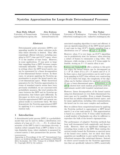
Nyström <strong>Approximation</strong> <strong>for</strong> <strong>Large</strong>-<strong>Scale</strong> <strong>Determinantal</strong> <strong>Processes</strong><br />
Raja Hafiz Affandi Alex Kulesza Emily B. Fox Ben Taskar<br />
University of Pennsylvania University of Michigan University of Washington University of Washington<br />
rajara@wharton.upenn.edu kulesza@umich.edu ebfox@stat.washington.edu taskar@cs.washington.edu<br />
Abstract<br />
<strong>Determinantal</strong> point processes (DPPs) are<br />
appealing models <strong>for</strong> subset selection problems<br />
where diversity is desired. They offer<br />
surprisingly efficient inference, including sampling<br />
in O(N 3 ) time and O(N 2 ) space, where<br />
N is the number of base items. However,<br />
in some applications, N may grow so large<br />
that sampling from a DPP becomes computationally<br />
infeasible. This is especially true<br />
in settings where the DPP kernel matrix cannot<br />
be represented by a linear decomposition<br />
of low-dimensional feature vectors. In these<br />
cases, we propose applying the Nyström approximation<br />
to project the kernel matrix into<br />
a low-dimensional space. While theoretical<br />
guarantees <strong>for</strong> the Nyström approximation in<br />
terms of standard matrix norms have been<br />
previously established, we are concerned with<br />
probabilistic measures, like total variation distance<br />
between the DPP and its Nyström approximation,<br />
that behave quite differently. In<br />
this paper we derive new error bounds <strong>for</strong> the<br />
Nyström-approximated DPP and present empirical<br />
results to corroborate them. We then<br />
demonstrate the Nyström-approximated DPP<br />
by applying it to a motion capture summarization<br />
task.<br />
1 Introduction<br />
A determinantal point process (DPP) is a probabilistic<br />
model that can be used to define a distribution over<br />
subsets of a base set Y = {1, . . . , N}. A critical characteristic<br />
of the DPP is that it encourages diversity: a<br />
random subset sampled from a DPP is likely to contain<br />
dissimilar items, where similarity is measured by<br />
a kernel matrix L that parametrizes the process. The<br />
Appearing in Proceedings of the 16 th International Conference<br />
on Artificial Intelligence and Statistics (AISTATS)<br />
2013, Scottsdale, AZ, USA. Volume 31 of JMLR: W&CP<br />
31. Copyright 2013 by the authors.<br />
associated sampling algorithm is exact and efficient; it<br />
uses an eigendecomposition of the DPP kernel matrix<br />
L and runs in time O(N 3 ) despite sampling from a<br />
distribution over 2 N subsets (Hough et al., 2006).<br />
However, when N is very large, an O(N 3 ) algorithm<br />
can be prohibitively slow; <strong>for</strong> instance, when selecting<br />
a subset of frames to summarize a long video. Furthermore,<br />
while storing a vector of N items might be<br />
feasible, storing an N × N matrix often is not.<br />
Kulesza and Taskar (2010) offer a solution to this problem<br />
when the kernel matrix can be decomposed as<br />
L = B ⊤ B, where B is a D × N matrix and D ≪ N.<br />
In these cases a dual representation can be used to per<strong>for</strong>m<br />
sampling in O(D 3 ) time without ever constructing<br />
L. If D is finite but large, the complexity of the algorithm<br />
can be further reduced by randomly projecting<br />
B into a lower-dimensional space. Gillenwater et al.<br />
(2012) showed how such random projections yield an<br />
approximate model with bounded variational error.<br />
However, linear decomposition of the kernel matrix<br />
using low-dimensional (or even finite-dimensional) features<br />
may not be possible. Even a simple Gaussian<br />
kernel has an infinite-dimensional feature space, and<br />
<strong>for</strong> many applications, including video summarization,<br />
the kernel can be even more complex and nonlinear.<br />
Here we address these computational issues by applying<br />
the Nyström method to approximate a DPP kernel<br />
matrix L as a low rank matrix ˜L. This approximation<br />
is based on a subset of the N items called landmarks;<br />
a small number of landmarks can often be sufficient to<br />
reproduce the bulk of the kernel’s eigenspectrum.<br />
The per<strong>for</strong>mance of adaptive Nyström methods has<br />
been well documented both empirically and theoretically.<br />
However, there are significant challenges in<br />
extending these results to the DPP. Most existing theoretical<br />
results bound the Frobenius or spectral norm<br />
of the kernel error matrix, but we show that these<br />
quantities are insufficient to give useful bounds on distributional<br />
measures like variational distance. Instead,<br />
we derive novel bounds <strong>for</strong> the Nyström approximation<br />
that are specifically tailored to DPPs, nontrivially
Nyström <strong>Approximation</strong> <strong>for</strong> <strong>Large</strong>-<strong>Scale</strong> <strong>Determinantal</strong> <strong>Processes</strong><br />
Algorithm 1 DPP-Sample(L)<br />
Input: kernel matrix L<br />
{(v n , λ n )} N n=1 ← eigendecomposition of L<br />
J ← ∅<br />
<strong>for</strong> n = 1, . . . , N do<br />
J ← J ∪ {n} with prob.<br />
V ← {v n } n∈J<br />
Y ← ∅<br />
while |V | > 0 do<br />
λ n<br />
λ n+1<br />
Select i from Y with Pr(i) = 1<br />
|V |<br />
∑v∈V (v⊤ e i ) 2<br />
Y ← Y ∪ {i}<br />
V ← V ⊥ei , an orthonormal basis <strong>for</strong> the subspace<br />
of V orthogonal to e i<br />
Output: Y<br />
characterizing the propagation of the approximation<br />
error through the structure of the process.<br />
Our bounds are provably tight in certain cases, and<br />
we demonstrate empirically that the bounds are in<strong>for</strong>mative<br />
<strong>for</strong> a wide range of real and simulated data.<br />
These experiments also show that the proposed method<br />
provides a close approximation <strong>for</strong> DPPs on large sets.<br />
Finally, we apply our techniques to select diverse and<br />
representative frames from a series of motion capture<br />
recordings. Based on a user survey, we find that the<br />
frames sampled from a Nyström-approximated DPP<br />
<strong>for</strong>m better summaries than randomly chosen frames.<br />
2 Background<br />
In this section we review the determinantal point process<br />
(DPP) and its dual representation.We then outline<br />
existing Nyström methods and theoretical results.<br />
2.1 <strong>Determinantal</strong> Point <strong>Processes</strong><br />
A random point process P on a discrete base set Y =<br />
{1, . . . , N} is a probability measure on the set 2 Y of<br />
all possible subsets of Y. For a positive semidefinite<br />
N × N kernel matrix L, the DPP, P L , is given by<br />
P L (A) = det(L A)<br />
det(L + I) , (1)<br />
where L A ≡ [L ij ] i,j∈A is the submatrix of L indexed<br />
by elements in A, and I is the N × N identity matrix.<br />
We use the convention det(L ∅ ) = 1. This L-ensemble<br />
<strong>for</strong>mulation of DPPs was first introduced by Borodin<br />
and Rains (2005). Hough et al. (2006) showed that<br />
sampling from a DPP can be done efficiently in O(N 3 ),<br />
as described in Algorithm 1.<br />
Algorithm<br />
In applications where diverse sets of a fixed size are<br />
desired, we can consider instead the kDPP (Kulesza<br />
and Taskar, 2011), which only gives positive probability<br />
to sets of a fixed cardinality k. The L-ensemble construction<br />
of a kDPP, denoted PL k , gives probabilities<br />
2 Dual-DPP-Sample(B)<br />
Input: B such that L = B ⊤ B.<br />
{(ˆv n , λ n )} N n=1 ← eigendecomposition of C = BB ⊤<br />
J ← ∅<br />
<strong>for</strong> n = 1, . . . , N do<br />
J ← J ∪ {n} with prob.<br />
{ }<br />
ˆv ˆV ← n<br />
√ˆv ⊤ C ˆv<br />
n∈J<br />
λ n<br />
λ n+1<br />
Y ← ∅<br />
while | ˆV | > 0 do<br />
Select i from Y with Pr(i) = 1<br />
| ˆV |<br />
∑ˆv∈ ˆV (ˆv⊤ B i ) 2<br />
Y ← Y ∪ {i}<br />
Let ˆv 0 be a vector in ˆV with Bi ⊤ˆv 0 ≠ 0<br />
Update ˆV<br />
{<br />
← ˆv − ˆv⊤ B i<br />
ˆv ˆv ⊤ 0 Bi 0 | ˆv ∈ ˆV<br />
}<br />
− {ˆv 0 }<br />
Orthonormalize ˆV w.r.t. 〈ˆv 1 , ˆv 2 〉 = ˆv ⊤ 1 Cˆv 2<br />
Output: Y<br />
P k L(A) =<br />
det(L A )<br />
∑|A ′ |=k det(L A ′) (2)<br />
<strong>for</strong> all sets A ⊆ Y with cardinality k. Kulesza and<br />
Taskar (2011) showed that kDPPs can be sampled<br />
with the same asymptotic efficiency as standard DPPs<br />
using recursive computation of elementary symmetric<br />
polynomials.<br />
2.2 Dual Representation of DPPs<br />
In special cases where L is a linear kernel of low dimension,<br />
Kulesza and Taskar (2010) showed that the<br />
complexity of sampling from these DPPs can be be<br />
significantly reduced. In particular, when L = B ⊤ B,<br />
with B a D × N matrix and D ≪ N, the complexity of<br />
the sampling algorithm can be reduced to O(D 3 ). This<br />
arises from the fact that L and the dual kernel matrix<br />
C = BB ⊤ share the same nonzero eigenvalues, and<br />
<strong>for</strong> each eigenvector v k of L, Bv k is the corresponding<br />
eigenvector of C. This leads to the sampling algorithm<br />
given in Algorithm 2, which takes time O(D 3 + ND)<br />
and space O(ND).<br />
2.3 Nyström Method<br />
For many applications, including SVM-based classification,<br />
Gaussian process regression, PCA, and, in<br />
our case, sampling DPPs, fundamental algorithms require<br />
kernel matrix operations of space O(N 2 ) and time<br />
O(N 3 ). A common way to improve scalability is to create<br />
a low-rank approximation to the high-dimensional<br />
kernel matrix. One such technique is known as the<br />
Nyström method, which involves selecting a small number<br />
of landmarks and then using them as the basis <strong>for</strong><br />
a low rank approximation.<br />
Given a sample W of l landmark items corresponding to<br />
a subset of the indices of an N × N symmetric positive
Raja Hafiz Affandi, Alex Kulesza, Emily B. Fox, Ben Taskar<br />
semidefinite matrix L, let W be the complement of W<br />
(with size N − l), let L W and L W<br />
denote the principal<br />
submatrices indexed by W and W , respectively, and<br />
let L W W<br />
denote the (N − l) × l submatrix of L with<br />
row indices from W and column indices from W . Then<br />
we can write L in block <strong>for</strong>m as<br />
( )<br />
LW L<br />
L = W W<br />
. (3)<br />
L W W<br />
L W<br />
If we denote the pseudo-inverse of L W as L + W<br />
, then the<br />
Nyström approximation of L using W is<br />
(<br />
LW L ˜L = W W<br />
L W W<br />
L W W<br />
L + W L W W<br />
)<br />
. (4)<br />
Fundamental to this method is the choice of W . Various<br />
techniques have been proposed; some have theoretical<br />
guarantees, while others have only been demonstrated<br />
empirically. Williams and Seeger (2001) first proposed<br />
choosing W by uni<strong>for</strong>m sampling without replacement.<br />
A variant of this approach was proposed by Frieze<br />
et al. (2004) and Drineas and Mahoney (2005), who<br />
sample W with replacement, and with probabilities<br />
proportional to the squared diagonal entries of L. This<br />
produces a guarantee that, with high probability,<br />
‖L − ˜L‖ 2 ≤ ‖L − L r ‖ 2 + ɛ<br />
N∑<br />
L 2 ii . (5)<br />
i=1<br />
where L r is the best rank-r approximation to L.<br />
Kumar et al. (2012) later proved that the same rate<br />
of convergence applies <strong>for</strong> uni<strong>for</strong>m sampling without<br />
replacement, and argued that uni<strong>for</strong>m sampling outper<strong>for</strong>ms<br />
other non-adaptive methods <strong>for</strong> many real-world<br />
problems while being computationally cheaper.<br />
2.4 Adaptive Nyström Method<br />
Instead of sampling elements of W from a fixed distribution,<br />
Deshpande et al. (2006) introduced the idea<br />
of adaptive sampling, which alternates between selecting<br />
landmarks and updating the sampling distribution<br />
<strong>for</strong> the remaining items. Intuitively, items whose kernel<br />
values are poorly approximated under the existing<br />
sample are more likely to be chosen in the next round.<br />
By sampling in each round landmarks W t chosen according<br />
to probabilities p (t)<br />
i ∝ ‖L i − ˜L i (W 1 ∪ · · · ∪<br />
W t−1 )‖ 2 2 (where L i denotes the ith column of L), we<br />
are guaranteed that<br />
E<br />
(‖L − ˜L(W<br />
)<br />
)‖ F ≤ ‖L − L r‖ F<br />
1 − ɛ<br />
∑<br />
N<br />
+ ɛ T L 2 ii . (6)<br />
i=1<br />
where L r is the best rank-r approximation to L and<br />
W = W 1 ∪ · · · ∪ W T .<br />
Algorithm 3 Nyström-based (k)DPP sampling<br />
Input: Chosen landmark indices W = {i 1 , . . . , i l }<br />
L ∗W ← N × l matrix <strong>for</strong>med by chosen landmarks<br />
L W ← principal submatrix of L indexed by W<br />
L + W ← pseudoinverse of L W<br />
B = (L ∗W ) ⊤ (L + W )1/2<br />
Y ← Dual-(k)DPP-Sample(B)<br />
Output: Y<br />
Kumar et al. (2012) argue that adaptive Nyström methods<br />
empirically outper<strong>for</strong>m the non-adaptive versions in<br />
cases where the number of landmarks is small relative<br />
to N. In fact, their results suggest that the per<strong>for</strong>mance<br />
gains of adaptive Nyström methods relative to<br />
the non-adaptive schemes are inversely proportional to<br />
the percentage of items chosen as landmarks.<br />
3 Nyström Method <strong>for</strong> DPP/kDPP<br />
As described in Section 2.2, a DPP whose kernel matrix<br />
has a known decomposition of rank D can be sampled<br />
using the dual representation, reducing the time complexity<br />
from O(N 3 ) to O(D 3 + ND) and the space<br />
complexity from O(N 2 ) to O(ND). However, in many<br />
settings such a decomposition may not be available, <strong>for</strong><br />
example if L is generated by infinite-dimensional features.<br />
In these cases we propose applying the Nyström<br />
approximation to L, building an l-dimensional approximation<br />
and applying the dual representation to reduce<br />
sampling complexity to O(l 3 + Nl) time and O(Nl)<br />
space (see Algorithm 3).<br />
To the best of our knowledge, analysis of the error of<br />
the Nyström approximation has been limited to the<br />
Frobenius and spectral norms of the residual matrix<br />
L − ˜L, and no bounds exist <strong>for</strong> volumetric measures<br />
of error which are more relevant <strong>for</strong> DPPs. The challenge<br />
here is to study how the Nyström approximation<br />
simultaneously affects all possible minors of L.<br />
In fact, a small error in the matrix norm can have a<br />
large effect on the minors of the matrix:<br />
Example 1. Consider matrices L = diag(M, . . . , M, ɛ)<br />
and ˜L = diag(M, . . . , M, 0) <strong>for</strong> some large M and small<br />
ɛ. Although ‖L − ˜L‖ F = ‖L − ˜L‖ 2 = ɛ, <strong>for</strong> any A that<br />
includes the final index, we have det(L A ) − det(˜L A ) =<br />
ɛM k−1 , where k = |A|.<br />
It is conceivable that while error on some subsets is<br />
large, most subsets are well approximated. Un<strong>for</strong>tunately,<br />
this not generally true.<br />
Definition 1. The variational distance between the<br />
DPP with kernel L and the DPP with the Nystromapproximated<br />
kernel ˜L is given by<br />
‖P L − P ˜L‖ 1 = 1 ∑<br />
|P L (A) − P ˜L(A)| . (7)<br />
2<br />
A∈2 Y
Nyström <strong>Approximation</strong> <strong>for</strong> <strong>Large</strong>-<strong>Scale</strong> <strong>Determinantal</strong> <strong>Processes</strong><br />
The variational distance is a natural global measure of<br />
approximation that ranges from 0 to 1. Un<strong>for</strong>tunately,<br />
it is not difficult to construct a sequence of matrices<br />
where the matrix norms of L − ˜L tend to zero but the<br />
variational distance does not.<br />
Example 2. Let L be a diagonal matrix with entries<br />
1/N and ˜L be a diagonal matrix with N/2 entries<br />
equal to 1/N and the rest equal to 0. Note that<br />
||L − ˜L|| F = 1/ √ 2N and ||L − ˜L|| 2 = 1/N, which<br />
tend to zero as N → ∞. However, the variational<br />
distance is bounded away from zero. To see this, note<br />
that the normalizers are det(L + I) = (1 + 1/N) N<br />
and<br />
√<br />
det(˜L + I) = (1 + 1/N) N/2 , which tend to e and<br />
e, respectively. Consider all subsets which have zero<br />
mass in the approximation, S = {A : det(˜L A ) = 0}.<br />
Summing up the unnormalized mass of sets in the complement<br />
of S, we have ∑ A/∈S det(L A) = det(˜L+I) and<br />
thus ∑ A∈S det(L A) = det(L + I) − det(˜L + I). Now<br />
consider the contribution of just the sets in S to the<br />
variational distance:<br />
‖P L − P ˜L‖ 1 ≥ 1 ∣<br />
∑<br />
det(L A ) ∣∣∣<br />
2 ∣det(L + I) − 0 (8)<br />
A∈S<br />
= det(L + I) − det(˜L + I)<br />
2 det(L + I)<br />
which tends to e−√ e<br />
2e<br />
≈ 0.1967 as N → ∞.<br />
, (9)<br />
One might still hope that pathological cases occur only<br />
<strong>for</strong> diagonal matrices, or more generally <strong>for</strong> matrices<br />
that have high coherence (Candes and Romberg, 2007).<br />
In fact, coherence has previously been used by Talwalkar<br />
and Rostamizadeh (2010) to analyze the error<br />
of the Nyström approximation. Define the coherence<br />
µ(L) = √ N max |v ij | , (10)<br />
i,j<br />
where each v i is a unit-norm eigenvector of L. A diagonal<br />
matrix achieves the highest coherence of √ N<br />
and a matrix with all entries equal to a constant<br />
has the lowest coherence of 1. Suppose that f(N)<br />
is a sublinear but monotone increasing function with<br />
lim N→∞ f(N) = ∞. We can construct a sequence of<br />
kernels L with µ(L) = √ f(N) = o( √ N) <strong>for</strong> which matrix<br />
norms of the Nyström approximation error tend to<br />
zero, but the variational distance tends to a constant.<br />
Example 3. Let L be a block diagonal matrix with<br />
f(N) constant blocks, each of size N/f(N), where each<br />
non-zero entry is 1/N. Let ˜L be structured like L<br />
except with half of the blocks set to zero. Note that<br />
µ 2 (L) = f(N) by construction and that each block<br />
1<br />
contributes a single eigenvalue of<br />
f(N)<br />
; the Frobenius<br />
and spectral norms of L − ˜L thus tend to zero as N<br />
increases. The DPP normalizers are given by det(L +<br />
I) = (1 + 1/f(N)) f(N) → e and det(˜L + I) = (1 +<br />
1/f(N)) f(N)/2 → √ e. By a similar argument to the<br />
one <strong>for</strong> diagonal matrices, we can show that variational<br />
distance tends to e−√ e<br />
2e .<br />
Un<strong>for</strong>tunately, in the cases above, the Nyström method<br />
will yield poor approximations to the original DPPs.<br />
Convergence of the matrix norm error alone is thus<br />
generally insufficient to obtain tight bounds on the<br />
resulting approximate DPP distribution. It turns out<br />
that the gap between the eigenvalues of the kernel<br />
matrix and the spectral norm error plays a major role<br />
in the effectiveness of the Nyström approximation <strong>for</strong><br />
DPPs, as we will show in Theorems 1 and 2. In the<br />
examples above, this gap is not large enough <strong>for</strong> a close<br />
approximation; in particular, the spectral norm errors<br />
are equal to the smallest non-zero eigenvalues. In the<br />
next subsection, we derive approximation bounds <strong>for</strong><br />
DPPs that are applicable to any landmark-selection<br />
scheme within the Nyström framework.<br />
3.1 Preliminaries<br />
We start with a result <strong>for</strong> positive semidefinite matrices<br />
known as Weyl’s inequality:<br />
Lemma 1. (Bhatia, 1997) Let L = ˜L + E, where L, ˜L<br />
and E are all positive semidefinite N ×N matrices with<br />
eigenvalues λ 1 ≥ . . . ≥ λ N ≥ 0, ˜λ 1 ≥ . . . ≥ ˜λ N ≥ 0,<br />
and ξ 1 ≥ . . . ≥ ξ N ≥ 0, respectively. Then<br />
λ n ≤ ˜λ m + ξ n−m+1 <strong>for</strong> m ≤ n , (11)<br />
λ n ≥ ˜λ m + ξ n−m+N <strong>for</strong> m ≥ n . (12)<br />
Going <strong>for</strong>ward, we use the convention λ i = 0 <strong>for</strong> i > N.<br />
Weyl’s inequality gives the following two corollaries.<br />
Corollary 1. When ξ j = 0 <strong>for</strong> j = r + 1, . . . , N, then<br />
<strong>for</strong> j = 1, . . . , N,<br />
λ j ≥ ˜λ j ≥ λ j+r . (13)<br />
Proof. For the first inequality, let n = m = j in (12).<br />
For the second, let m = j and n = j + r in (11).<br />
Corollary 2. For j = 1, . . . , N,<br />
λ j − ξ N ≥ ˜λ j ≥ λ j − ξ 1 . (14)<br />
Proof. We let n = m = j in (11) and (12), then rearrange<br />
terms to get the desired result.<br />
The following two lemmas pertain specifically to the<br />
Nyström method.<br />
Lemma 2. (Arcolano, 2011) Let ˜L be a Nyström approximation<br />
of L. Let E = L − ˜L be the corresponding<br />
error matrix. Then E is positive semidefinite with<br />
rank(E) = rank(L) − rank(˜L).
Raja Hafiz Affandi, Alex Kulesza, Emily B. Fox, Ben Taskar<br />
Lemma 3. Denote the set of indices of the chosen<br />
landmarks in the Nyström construction as W . Then if<br />
A ⊆ W ,<br />
det(L A ) = det(˜L A ) . (15)<br />
Proof. L W = ˜L W and A ⊆ W ; the result follows.<br />
3.2 Set-wise bounds <strong>for</strong> DPPs<br />
We are now ready to state set-wise bounds on the<br />
Nyström approximation error <strong>for</strong> DPPs and kDPPs.<br />
In particular, <strong>for</strong> each set A ⊆ Y, we want to bound<br />
the probability gap |P L (A) − P ˜L(A)|. Going <strong>for</strong>ward,<br />
we use P A ≡ P L (A) and ˜P A ≡ P ˜L(A).<br />
Once again, we denote the set of all sampled landmarks<br />
as W . We first consider the case where A ⊆ W . In<br />
this case, by Lemma 3, det(L A ) = det(˜L A ). Thus<br />
the only error comes from the normalization term in<br />
Equation (1). Theorem 1 gives the desired bound.<br />
Theorem 1. Let λ 1 ≥ . . . ≥ λ N be the eigenvalues of<br />
L. If ˜L has rank r, L has rank m, and<br />
ˆλ i = max<br />
{λ i+(m−r) , λ i − ‖L − ˜L‖<br />
}<br />
2 , (16)<br />
then <strong>for</strong> A ⊆ W ,<br />
[ ∏n ]<br />
|P A − ˜P i=1 A | ≤ P (1 + λ i)<br />
A ∏ n<br />
i=1 (1 + ˆλ i ) − 1<br />
. (17)<br />
Proof.<br />
[<br />
]<br />
|P A − ˜P det(˜L A )<br />
A | =<br />
det(˜L + I) − det(L A)<br />
(18)<br />
det(L + I)<br />
[ ] [ ∏n ]<br />
det(L + I)<br />
=P A<br />
det(˜L + I) − 1 i=1<br />
= P (1 + λ i)<br />
A ∏ n<br />
i=1 (1 + ˜λ i ) − 1 ,<br />
where ˜λ 1 ≥, . . . , ˜λ N ≥ 0 represent the eigenvalues of ˜L.<br />
The first equality follows from the fact that λ i ≥ ˜λ i ,<br />
due to the first inequality in Corollary 1. Now note<br />
that since L = ˜L + E, by Lemma 2, Corollary 1, and<br />
Corollary 2 we have<br />
˜λ i ≥ λ i+(m−r) , ˜λi ≥ λ i − ξ 1 = λ i − ‖L − ˜L‖ 2 . (19)<br />
The theorem follows.<br />
For A ⊈ W , we must also account <strong>for</strong> error in the<br />
numerator, since it is not generally true that det(L A ) =<br />
det(˜L A ). Theorem 2 gives a set-wise probability bound.<br />
Theorem 2. Assume ˜L has rank r, L has rank m,<br />
|A| = k, and L A has eigenvalues λ A 1 ≥ . . . ≥ λ A k . Let<br />
ˆλ i = max<br />
{λ i+(m−r) , λ i − ‖L − ˜L‖<br />
}<br />
2 (20)<br />
{<br />
= max λ A i − ‖L − ˜L‖<br />
}<br />
2 , 0 . (21)<br />
ˆλ A i<br />
Then <strong>for</strong> A ⊈ W ,<br />
|P A − ˜P A | (22)<br />
{[ ∏ k<br />
i=1<br />
≤ P A max 1 −<br />
ˆλ<br />
] [ ∏n ]}<br />
A<br />
i i=1<br />
,<br />
(1 + λ i)<br />
∏ n<br />
i=1 (1 + ˆλ i ) − 1 .<br />
Proof.<br />
∏ k<br />
i=1 λA i<br />
[<br />
]<br />
det(L + I) det(˜L A )<br />
˜P A − P A = P A<br />
det(˜L + I) det(L A ) − 1<br />
= P A<br />
[( ∏n<br />
i=1 (1 + λ i)<br />
∏ n<br />
i=1 (1 + ˜λ i )<br />
) ( ∏k<br />
i=1 ˜λ A i<br />
∏ k<br />
i=1 λA i<br />
)<br />
− 1<br />
(23)<br />
Here ˜λ A 1 , ≥, . . . , ≥ ˜λ A k<br />
are the eigenvalues of ˜L A . Now<br />
note that L A = ˜L A + E A . Since E is positive semidefinite,<br />
E A is also positive semidefinite. Thus by Corollary<br />
1 we have λ A i ≥ ˜λ A i , and so<br />
[ ∏n ]<br />
i=1 ˜P A − P A ≤ P (1 + λ i)<br />
A ∏ n<br />
i=1 (1 + ˆλ i ) − 1 . (24)<br />
For the reverse inequality, we multiply Equation (23)<br />
by -1 and use the fact that λ i ≥ ˜λ i and λ A i ≥ 0. By<br />
Corrolary 2,<br />
˜λ A i ≥ λ A i − ξ A 1 ≥ λ A i − ξ 1 = λ A i − ‖L − ˜L‖ 2 , (25)<br />
resulting in the inequality<br />
∏ k<br />
P A − ˜P i=1 A ≤ P A<br />
[1 −<br />
ˆλ<br />
]<br />
A<br />
i<br />
. (26)<br />
∏ k<br />
i=1 λA i<br />
The theorem follows by combining the two inequalities.<br />
Both theorems are tight if the approximation is exact<br />
(‖L− ˜L‖ 2 = 0). It can also be shown that these bounds<br />
are tight <strong>for</strong> the diagonal matrix examples discussed at<br />
the beginning of this section, where the spectral norm<br />
error is equal to the non-zero eigenvalues. Moreover,<br />
these bounds are convenient since they are expressed<br />
in terms of the spectral norm of the error matrix and<br />
there<strong>for</strong>e can be easily combined with existing approximation<br />
bounds <strong>for</strong> the Nyström method. Note that<br />
the eigenvalues of L and the size of the set A both<br />
play important roles in the bound. In fact, these two<br />
quantities are closely related; it is possible to show that<br />
the expected size of a set sampled from a DPP is<br />
E [|A|] =<br />
N∑<br />
n=1<br />
]<br />
λ n<br />
λ n + 1 . (27)<br />
Thus, if L has large eigenvalues, we expect the Nyström<br />
approximation error to be large as well since the DPP<br />
associated with L gives high probability to large sets.<br />
.
Nyström <strong>Approximation</strong> <strong>for</strong> <strong>Large</strong>-<strong>Scale</strong> <strong>Determinantal</strong> <strong>Processes</strong><br />
3.3 Set-wise bounds <strong>for</strong> kDPPs<br />
We can obtain similar results <strong>for</strong> Nyströmapproximated<br />
kDPPs. In this case, <strong>for</strong> each set<br />
A with |A| = k we want to bound the probability gap<br />
|PA k − ˜P A k |. Using Equation (2) <strong>for</strong> Pk A , it is easy to<br />
generalize the theorems in the preceding section. The<br />
proofs <strong>for</strong> the following theorems are provided in the<br />
supplementary material.<br />
Theorem 3. Let e k denote the kth elementary symmetric<br />
polynomial of L:<br />
e k (λ 1 , . . . , λ N ) = ∑ ∏<br />
λ n . (28)<br />
|J|=k n∈J<br />
Under the conditions of Theorem 1, <strong>for</strong> A ⊆ W ,<br />
[<br />
]<br />
|PA k − ˜P A| k ≤ PA<br />
k e k (λ 1 , . . . , λ N )<br />
e k (ˆλ 1 , . . . , ˆλ N ) − 1 . (29)<br />
Theorem 4. Under the conditions of Theorem 2, <strong>for</strong><br />
A ⊈ W ,<br />
|PA k − ˜P A| k (30)<br />
{[<br />
] [ ∏ k<br />
≤ PA k e k (λ 1 , . . . , λ N )<br />
max<br />
e k (ˆλ 1 , . . . , ˆλ N ) − 1 i=1<br />
, 1 −<br />
ˆλ<br />
]}<br />
A<br />
i<br />
.<br />
∏ k<br />
i=1 λA i<br />
Note that the scale of the eigenvalues has no effect on<br />
the kDPP; we can directly observe from Equation (2)<br />
that scaling L does not change the kDPP distribution<br />
since any constant factor appears to the kth power in<br />
both the numerator and denominator.<br />
4 Empirical Results<br />
In this section we present empirical results on the<br />
per<strong>for</strong>mance of the Nyström approximation <strong>for</strong> kDPPs<br />
using three datasets small enough <strong>for</strong> us to per<strong>for</strong>m<br />
ground-truth inference in the original kDPP. Two of<br />
the datasets are derived from real-world applications<br />
available on the UCI repository 1 —the first is a linear<br />
kernel matrix constructed from 1000 MNIST images,<br />
and the second an RBF kernel matrix constructed<br />
from 1000 Abalone data points—while the third is<br />
synthetic and comprises a 1000 × 1000 diagonal kernel<br />
matrix with exponentially decaying diagonal elements.<br />
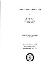
Figure 1 displays the log-eigenvalues <strong>for</strong> each dataset.<br />
On each dataset, we per<strong>for</strong>m the Nyström approximation<br />
with three different sampling schemes: stochastic<br />
adaptive, greedy adaptive, and uni<strong>for</strong>m. The stochastic<br />
adaptive sampling technique is a simplified version of<br />
the scheme used in Deshpande et al. (2006), where,<br />
on each iteration of landmark selection, we update<br />
E = L − ˜L and then sample landmarks with probabilities<br />
proportional to Eii 2 . In the greedy scheme,<br />
1 http://archive.ics.uci.edu/ml/<br />
log of eiganvalues<br />
10<br />
5<br />
0<br />
−5<br />
−10<br />
−15<br />
MNIST<br />
Abalone<br />
Artificial<br />
−20<br />
0 100 200 300 400 500 600<br />
i<br />
Figure 1: The first 600 log-eigenvalues <strong>for</strong> each dataset.<br />
we per<strong>for</strong>m a similar update, but always choose the<br />
landmarks with the maximum diagonal value E ii . Finally,<br />
<strong>for</strong> the uni<strong>for</strong>m method, we simply sample the<br />
landmarks uni<strong>for</strong>mly without replacement.<br />
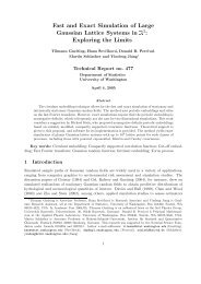
In Figure 2 (top), we plot log ||L− ˜L|| 2 <strong>for</strong> each dataset<br />
as a function of the number of landmarks sampled.<br />
For the MNIST data all sampling algorithms initially<br />
per<strong>for</strong>m equally well, but uni<strong>for</strong>m sampling becomes<br />
relatively worse after about 550 landmarks are sampled.<br />
For the Abalone data the adaptive methods<br />
per<strong>for</strong>m much better than uni<strong>for</strong>m sampling over the<br />
entire range of sampled landmarks. This phenomenon<br />
is perhaps explained by the analysis of Talwalkar and<br />
Rostamizadeh (2010), which suggests that uni<strong>for</strong>m<br />
sampling works well <strong>for</strong> the MNIST data due to its relatively<br />
low coherence (µ(L) = 0.5 √ N), while per<strong>for</strong>ming<br />
poorly on the higher-coherence Abalone dataset<br />
(µ(L) = 0.8 √ N). For both of the UCI datasets, the<br />
stochastic and greedy adaptive methods per<strong>for</strong>m similarly.<br />
However, <strong>for</strong> our artificial dataset it is easy to<br />
see that the greedy adaptive scheme is optimal since it<br />
chooses the top remaining eigenvalues in each iteration.<br />
In Figure 2 (bottom), we plot log ||P − ˜P || 1 <strong>for</strong> k = 10<br />
(estimated by sampling), as well as the theoretical<br />
bounds from Section 3. The bounds track the actual<br />
variational error closely <strong>for</strong> both the MNIST and<br />
Abalone datasets. For the artificial dataset uni<strong>for</strong>m<br />
sampling can do arbitrarily poorly, so we see looser<br />
bounds in this case. We note that the variational distance<br />
correlates strongly with the spectral norm error<br />
<strong>for</strong> each dataset.<br />
4.1 Related methods<br />
The Nystöm technique is, of course, not the only possible<br />
means of finding low-rank kernel approximations.<br />
One alternative <strong>for</strong> shift-invariant kernels is random<br />
Fourier features (RFFs), which were recently proposed<br />
by Rahimi and Recht (2007). RFFs map each item<br />
onto a random direction drawn from the Fourier trans<strong>for</strong>m<br />
of the kernel function; this results in a uni<strong>for</strong>m<br />
approximation of the kernel matrix. In practice, however,<br />
reasonable RFF approximations seem to require
Raja Hafiz Affandi, Alex Kulesza, Emily B. Fox, Ben Taskar<br />
log of spectral norm of error matrix<br />
4<br />
2<br />
0<br />
−2<br />
−4<br />
−6<br />
−8<br />
Uni<strong>for</strong>m<br />
Stochastic<br />
Greedy<br />
−10<br />
100 200 300 400 500 600<br />
Number of columns sampled<br />
log of spectral norm of error matrix<br />
4<br />
2<br />
0<br />
−2<br />
−4<br />
−6<br />
−8<br />
Uni<strong>for</strong>m<br />
Stochastic<br />
Greedy<br />
−10<br />
100 200 300 400 500 600<br />
Number of columns sampled<br />
log of spectral norm of error matrix<br />
4<br />
2<br />
0<br />
−2<br />
−4<br />
−6<br />
−8<br />
Uni<strong>for</strong>m<br />
Stochastic<br />
Greedy<br />
−10<br />
100 200 300 400 500 600<br />
Number of columns sampled<br />
log of L1 variation distance<br />
10<br />
5<br />
0<br />
−5<br />
−10<br />
Uni<strong>for</strong>m<br />
Stochastic<br />
Greedy<br />
−15<br />
100 200 300 400 500 600<br />
Number of columns sampled<br />
log of L1 variation distance<br />
10<br />
5<br />
0<br />
−5<br />
−10 Uni<strong>for</strong>m<br />
Stochastic<br />
Greedy<br />
−15<br />
100 200 300 400 500 600<br />
Number of columns sampled<br />
log of L1 variation distance<br />
50<br />
40<br />
30<br />
20<br />
10<br />
0<br />
Uni<strong>for</strong>m<br />
Stochastic<br />
Greedy<br />
−10<br />
100 200 300 400 500 600<br />
Number of columns sampled<br />
Figure 2: Error of Nyström approximations. Top: log(‖L − ˜L‖ 2 ) as a function of number of landmarks sampled.<br />
Bottom: log(‖P − ˜P‖ 1 ) as a function of number of landmarks sampled. The dashed lines show the bounds derived<br />
in Sec 3. From left to right, the datasets used are MNIST, Abalone and Artificial.<br />
log of L1 variation distance<br />
0<br />
−2<br />
−4<br />
−6<br />
−8<br />
−10<br />
−12<br />
−14<br />
Uni<strong>for</strong>m<br />
Random Fourier<br />
Stochastic<br />
Greedy<br />
−16<br />
100 200 300 400 500 600<br />
Number of sampled columns/features<br />
Figure 3: Error of Nyström and random Fourier features<br />
approximations on Abalone data: log(‖P − ˜P‖ 1 )<br />
as a function of the number of landmarks or random<br />
features sampled.<br />
a large number of random features, which can reduce<br />
the computational benefits of this technique.<br />
We per<strong>for</strong>med empirical comparisons between the<br />
Nyström methods and random Fourier features (RFFs)<br />
by approximating DPPs on the Abalone dataset. While<br />
RFFs generally match or outper<strong>for</strong>m uni<strong>for</strong>m sampling<br />
of Nyström landmarks, they result in significantly<br />
higher error compared to the adaptive versions, especially<br />
when there is high correlation between items, as<br />
shown in Figure 3. These results are consistent with<br />
those previously reported <strong>for</strong> kernel learning (Yang<br />
et al., 2012), where the Nyström method was shown<br />
to per<strong>for</strong>m significantly better in the presence of large<br />
eigengaps. We provide a more detailed empirical comparison<br />
with RFFs in the supplementary material.<br />
5 Experiments<br />
Finally, we demonstrate the Nyström approximation on<br />
a motion summarization task that is too large to permit<br />
tractable inference in the original DPP. As input, we<br />
are given a series of motion capture recordings, each<br />
of which depicts human subjects per<strong>for</strong>ming motions<br />
related to a particular activity, such as dancing or playing<br />
basketball. In order to aid browsing and retrieval of<br />
these recordings in the future, we would like to choose,<br />
from each recording, a small number of frames that<br />
summarize its motions in a visually intuitive way. Since<br />
a good summary should contain a diverse set of frames,<br />
a DPP is a natural model <strong>for</strong> this task.<br />
We obtained test recordings from the CMU motion<br />
capture database 2 , which offers motion captures of<br />
over 100 subjects per<strong>for</strong>ming a variety of actions. Each<br />
capture involves 31 sensors attached to the subject’s<br />
body and sampled 120 times per second. For each of<br />
nine activity categories—basketball, boxing, dancing,<br />
exercise, jumping, martial arts, playground, running,<br />
and soccer—we made a large input recording by concatenating<br />
all available captures in that category. On<br />
average, the resulting recordings are about N = 24,000<br />
frames long (min 3,358; max 56,601). At this scale,<br />
storage of a full N × N DPP kernel matrix would be<br />
highly impractical (requiring up to 25GB of memory),<br />
and O(N 3 ) SVD would be prohibitively expensive.<br />
In order to model the summarization problem as a DPP,<br />
we designed a simple kernel to measure the similarity<br />
between pairs of poses recorded in different frames. We<br />
first computed the variance <strong>for</strong> the location of each<br />
2 http://mocap.cs.cmu.edu/
Nyström <strong>Approximation</strong> <strong>for</strong> <strong>Large</strong>-<strong>Scale</strong> <strong>Determinantal</strong> <strong>Processes</strong><br />
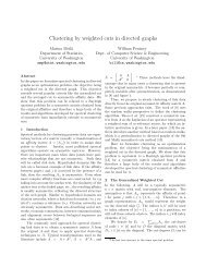
Figure 4: A sample pair of frame sets <strong>for</strong> the activity basketball. The top set is chosen randomly, while the<br />
bottom is sampled from the Nyström-approximated DPP.<br />
sensor <strong>for</strong> each activity; this allowed us to tailor the<br />
kernel to the specific motion being summarized. For<br />
instance, we might expect a high variance <strong>for</strong> foot<br />
locations in dancing, and a relatively smaller variance<br />
in boxing. We then used these variance measurements<br />
to specify a Gaussian kernel over the position of each<br />
sensor, and finally combined the Gaussian kernels with<br />
a set of weights chosen manually to approximately<br />
reflect the importance of each sensor location to human<br />
judgments of pose similarity. Specifically, <strong>for</strong> poses<br />
A = (a 1 , a 2 , . . . , a 31 ) and B = (b 1 , b 2 , . . . , b 31 ), where<br />
a 1 is the three dimensional location of the first sensor<br />
in pose A, etc., the kernel value is given by<br />
∑31<br />
(<br />
L(A, B) = w i exp − ‖a i − b i ‖ 2 )<br />
2<br />
2σi<br />
2 , (31)<br />
i=1<br />
where σi<br />
2 is the variance measured <strong>for</strong> sensor i, and<br />
w = (w 1 , w 2 , . . . , w 31 ) is the importance weight vector.<br />
We chose a weight of 1 <strong>for</strong> the head, wrists, and ankles,<br />
a weight of 0.5 <strong>for</strong> the elbows and knees, and a weight<br />
of 0 <strong>for</strong> the remaining 22 sensors.<br />
This kind of spatial kernel is natural <strong>for</strong> this task,<br />
where the items have inherent geometric relationships.<br />
However, because the feature representation is infinitedimensional,<br />
it does not readily admit use of the dual<br />
methods of Kulesza and Taskar (2010). Instead, we<br />
applied the stochastic adaptive Nyström approximation<br />
developed above, sampling a total of 200 landmark<br />
frames from each recording in 20 iterations (10 frames<br />
per iteration), bringing the intractable task of sampling<br />
from the high dimensional DPP down to an easily<br />
manageable size: sampling a set of ten summary frames<br />
from the longest recording took less than one second.<br />
Of course, this speedup naturally comes at some approximation<br />
cost. In order to evaluate empirically<br />
whether the Nyström samples retained the advantages<br />
of the original DPP, which is too expensive <strong>for</strong> direct<br />
comparison, we per<strong>for</strong>med a user study. Each subject<br />
in the study was shown, <strong>for</strong> each of the original nine<br />
recordings, a set of ten poses (rendered graphically)<br />
sampled from the approximated DPP model alongside<br />
a set of ten poses sampled uni<strong>for</strong>mly at random (see<br />
Evaluation measure % DPP % Random<br />
Quality 66.7 33.3<br />
Diversity 64.8 35.2<br />
Overall 67.3 32.7<br />
Table 1: The percentage of subjects choosing each<br />
method in a user study of motion capture summaries.<br />
Figure 4). We asked the subjects to evaluate the two<br />
pose sets with respect to the motion capture recording,<br />
which was provided in the <strong>for</strong>m of a rendered video.<br />
The subjects chose the set they felt better represented<br />
the characteristic poses from the video (quality), the<br />
set they felt was more diverse, and the set they felt<br />
made the better overall summary. The order of the two<br />
sets was randomized, and the samples were different<br />
<strong>for</strong> each user. 18 subjects completed the study, <strong>for</strong> a<br />
total of 162 responses to each question.<br />
The results of the user study are shown in Table 1.<br />
Overall, the subjects felt that the samples from the<br />
Nyström-approximated DPP were significantly better<br />
on all three measures, p < 0.001.<br />
6 Conclusion<br />
The Nyström approximation is an appealing technique<br />
<strong>for</strong> managing the otherwise intractable task of sampling<br />
from high-dimensional DPPs. We showed that this<br />
appeal is theoretical as well as practical: we proved<br />
upper bounds <strong>for</strong> the variational error of Nyströmapproximated<br />
DPPs and presented empirical results to<br />
validate them. We also demonstrated that Nyströmapproximated<br />
DPPs can be usefully applied to the task<br />
of summarizing motion capture recordings. Future<br />
work includes incorporating the structure of the kernel<br />
matrix to derive potentially tighter bounds.<br />
Acknowledgements<br />
RHA and EBF were supported in part by AFOSR<br />
Grant FA9550-12-1-0453 and DARPA Grant FA9550-<br />
12-1-0406 negotiated by AFOSR. BT was partially<br />
supported by NSF CAREER Grant 1054215 and by<br />
STARnet, a Semiconductor Research Corporation program<br />
sponsored by MARCO and DARPA.
Raja Hafiz Affandi, Alex Kulesza, Emily B. Fox, Ben Taskar<br />
References<br />
N.F. Arcolano. <strong>Approximation</strong> of Positive Semidefinite<br />
Matrices Using the Nyström Method. PhD thesis,<br />
Harvard University, 2011.<br />
R. Bhatia. Matrix Analysis, volume 169. Springer<br />
Verlag, 1997.<br />
A. Borodin and E.M. Rains. Eynard-Mehta Theorem,<br />
Schur Process, and Their Pfaffian Analogs. Journal<br />
of Statistical Physics, 121(3):291–317, 2005.<br />
E. Candes and J. Romberg. Sparsity and Incoherence<br />
in Compressive Sampling. Inverse Problems, 23(3):<br />
969, 2007.<br />
A. Deshpande, L. Rademacher, S. Vempala, and<br />
G. Wang. Matrix <strong>Approximation</strong> and Projective Clustering<br />
via Volume Sampling. Theory of Computing, 2:<br />
225–247, 2006.<br />
P. Drineas and M. W. Mahoney. On the Nyström<br />
Method <strong>for</strong> Approximating a Gram Matrix <strong>for</strong> Improved<br />
Kernel-based Learning. Journal of Machine<br />
Learning Research, 6:2153–2175, 2005.<br />
A. Frieze, R. Kannan, and S. Vempala. Fast Monte-<br />
Carlo Algorithms <strong>for</strong> Finding Low-rank <strong>Approximation</strong>s.<br />
Journal of the ACM (JACM), 51(6):1025–1041,<br />
2004.<br />
J. Gillenwater, A. Kulesza, and B. Taskar. Discovering<br />
Diverse and Salient Threads in Document Collections.<br />
Proceedings of the 2012 Joint Conference on Empirical<br />
Methods in Natural Language Processing and Computational<br />
Natural Language Learning, pages 710–720,<br />
2012.<br />
J.B. Hough, M. Krishnapur, Y. Peres, and B. Virág.<br />
<strong>Determinantal</strong> <strong>Processes</strong> and Independence. Probability<br />
Surveys, 3:206–229, 2006.<br />
A. Kulesza and B. Taskar. Structured <strong>Determinantal</strong><br />
Point <strong>Processes</strong>. Advances in Neural In<strong>for</strong>mation<br />
Processing Systems, 23:1171–1179, 2010.<br />
A. Kulesza and B. Taskar. k-DPPs: Fixed-size <strong>Determinantal</strong><br />
Point <strong>Processes</strong>. Proceedings of the 28th<br />
International Conference on Machine Learning, pages<br />
1193–1200, 2011.<br />
S. Kumar, M. Mohri, and A. Talwalkar. Sampling<br />
Methods <strong>for</strong> the Nyström Method. Journal of Machine<br />
Learning Research, 13:981–1006, 2012.<br />
A. Rahimi and B. Recht. Random Features <strong>for</strong> <strong>Large</strong>scale<br />
Kernel Machines. Advances in Neural In<strong>for</strong>mation<br />
Processing Systems, 20:1177–1184, 2007.<br />
A. Talwalkar and A. Rostamizadeh. Matrix Coherence<br />
and the Nyström Method. arXiv preprint<br />
arXiv:1004.2008, 2010.<br />
C. Williams and M. Seeger. Using the Nyström<br />
Method to Speed Up Kernel Machines. Advances in<br />
Neural In<strong>for</strong>mation Processing Systems, 13:682–688,<br />
2001.<br />
Ti. Yang, Y. Li, M. Mahdavi, R. Jin, and Z. Zhou.<br />
Nystrom Method vs Random Fourier Features: A<br />
Theoretical and Empirical Comparison. Advances in<br />
Neural In<strong>for</strong>mation Processing Systems, 25:485–493,<br />
2012.
Nyström <strong>Approximation</strong> <strong>for</strong> <strong>Large</strong>-<strong>Scale</strong> <strong>Determinantal</strong> <strong>Processes</strong><br />
A<br />
Appendix-Supplementary Material<br />
A.1 Proofs to Theorem 5 and Theorem 6<br />
Lemma 4. Let e k denote the kth elementary symmetric polynomial of L:<br />
e k (λ 1 , . . . , λ N ) = ∑ ∏<br />
λ n , (32)<br />
|J|=k n∈J<br />
and<br />
ˆλ i = max<br />
{λ i+(m−r) , λ i − ‖L − ˜L‖<br />
}<br />
2<br />
, (33)<br />
where m is the rank of L and r is the rank of ˜L. Then<br />
e k (λ 1 , . . . , λ N ) ≥ e k (˜λ 1 , . . . , ˜λ N ) ≥ e k (ˆλ 1 , . . . , ˆλ N ) . (34)<br />
Proof.<br />
by Corollary 1.<br />
On the other hand,<br />
e k (λ 1 , . . . , λ N ) = ∑ ∏<br />
λ n ≥ ∑ ∏<br />
˜λ n = e k (˜λ 1 , . . . , ˜λ N ) ,<br />
|J|=k n∈J |J|=k n∈J<br />
e k (˜λ 1 , . . . , ˜λ N ) = ∑ ∏<br />
˜λ n ≥ ∑ ∏<br />
ˆλ n = e k (ˆλ 1 , . . . , ˆλ N ) ,<br />
|J|=k n∈J |J|=k n∈J<br />
by Corollary 1 and Corollary 2.<br />
Since<br />
PL(A) k det(L A )<br />
= ∑<br />
|A ′ |=k det(L A ′) = det(L A )<br />
∑ ∏<br />
|J|=k<br />
using Lemma 4, we can now prove Theorem 3 and Theorem 4.<br />
n∈J λ n<br />
=<br />
det(L A )<br />
e k (λ 1 , . . . , λ N ) , (35)<br />
Proof of Theorem 3.<br />
[<br />
]<br />
|PA k − ˜P A| k det(˜L A )<br />
=<br />
e k (˜λ 1 , . . . , ˜λ N ) − det(L A )<br />
= PA<br />
k e k (λ 1 , . . . , λ N )<br />
where the last inequality follows from Lemma 4.<br />
[ ] [<br />
]<br />
ek (λ 1 , . . . , λ N )<br />
e k (˜λ 1 , . . . , ˜λ N ) − 1 ≤ PA<br />
k e k (λ 1 , . . . , λ N )<br />
e k (ˆλ 1 , . . . , ˆλ N ) − 1<br />
,<br />
Proof of Theorem 4.<br />
˜P k A − P k A = P k A<br />
[<br />
]<br />
e k (λ 1 , . . . , λ N ) det(˜L A )<br />
e k (˜λ 1 , . . . , ˜λ N ) det(L A ) − 1 = PA<br />
k<br />
[ (ek<br />
(λ 1 , . . . , λ N )<br />
e k (˜λ 1 , . . . , ˜λ N )<br />
) ( ∏ k<br />
i=1 ˜λ A i<br />
∏ k<br />
i=1 λA i<br />
)<br />
− 1<br />
]<br />
.<br />
Here ˜λ A 1 , ≥, . . . , ≥ ˜λ A k<br />
are the eigenvalues of ˜L A . Now note that L A = ˜L A + E A . Since E is positive semidefinite,<br />
it follows that E A is also positive semidefinite. Thus by Corollary 1, we have λ A i ≥ ˜λ A i and so<br />
[ ] [<br />
]<br />
˜P A k − PA k ≤ PA<br />
k ek (λ 1 , . . . , λ N )<br />
e k (˜λ 1 , . . . , ˜λ N ) − 1 ≤ PA<br />
k e k (λ 1 , . . . , λ N )<br />
e k (ˆλ 1 , . . . , ˆλ N ) − 1 ,<br />
where the last inequality follows from Lemma 4.<br />
On the other hand,<br />
[ ( ) ( ∏ k<br />
PA k − ˜P A k = PA<br />
k ek (λ 1 , . . . , λ N )<br />
1 −<br />
˜λ<br />
e k (˜λ 1 , . . . , ˜λ<br />
i=1 A i<br />
∏<br />
N ) k<br />
i=1 λA i<br />
)]<br />
. (36)
Raja Hafiz Affandi, Alex Kulesza, Emily B. Fox, Ben Taskar<br />
By Corrolary 2,<br />
˜λ A i ≥ λ A i − ξ A 1 ≥ λ A i − ξ 1 = λ A i − ‖L − ˜L‖ 2 . (37)<br />
We also note that ˜λ A i<br />
≥ 0. Since e k (λ 1 , . . . , λ N ) ≥ e k (˜λ 1 , . . . , ˜λ N ) by Lemma 4, we have<br />
[ ∏ k<br />
PA k − ˜P A k ≤ PA<br />
k i=1<br />
1 −<br />
ˆλ<br />
]<br />
A<br />
i<br />
. (38)<br />
∏ k<br />
i=1 λA i<br />
The theorem follows by combining the two inequalities.<br />
A.2 Empirical Comparisons to Random Fourier Features<br />
In cases where the kernel matrix L is generated from a shift-invariant kernel function k(x, y) = k(x − y), we<br />
can construct a low-rank approximation using random Fourier features (RFFs) (Rahimi and Recht, 2007). This<br />
involves mapping each data point x ∈ R d onto a random direction ω drawn from the Fourier trans<strong>for</strong>m of the<br />
kernel function. In particular, we draw ω ∼ p(ω), where<br />
∫<br />
p(ω) = k(∆) exp(−iω ⊤ ∆)d∆ , (39)<br />
R d<br />
draw b uni<strong>for</strong>mly from [0, 2π], and set z ω (x) = √ 2 cos(ω ⊤ x + b). It can be shown then that z ω (x)z ω (y) is an<br />
unbiased estimator of k(x − y). Note that the shift-invariant property of the kernel function is crucial to ensure<br />
that p(ω) is a valid probability distribution, due to Bochner’s Theorem. The variance of the estimate can be<br />
improved by drawing D random direction, ω 1 , . . . , ω D ∼ p(ω) and estimating the kernel function with k(x − y)<br />
as 1 D<br />
∑ D<br />
j=1 z ω j<br />
(x)z ωj (y).<br />
To use RFFs <strong>for</strong> approximating DPP kernel matrices, we assume that the matrix L is generated from a shiftinvariant<br />
kernel function, so that if x i is the vector representing item i then<br />
We construct a D × N matrix B with<br />
L ij = k(x i − x j ) . (40)<br />
B ij = 1 √<br />
D<br />
z ωi (x j ) i = 1, . . . , D, j = 1, . . . , N . (41)<br />
An unbiased estimator of the kernel matrix L is now given by ˜L RFF = B ⊤ B. Furthermore, note that an<br />
approximation to the dual kernel matrix C is given by ˜C RFF = BB ⊤ ; this allows use of the sampling algorithm<br />
given in Algorithm 2.<br />
We apply the RFF approximation method to the Abalone data from Section 4. We use a Gaussian RBF kernel,<br />
L ij = exp(− ‖x i − x j ‖ 2<br />
σ 2 ) i, j = 1, . . . , 1000 , (42)<br />
with σ 2 taking values 0.1,1, and 10. In this case, the Fourier trans<strong>for</strong>m of the kernel function, p(ω) is also a<br />
multivariate Gaussian.<br />
In Figure 5 we plot the empirically estimated log(‖P k − ˜P k ‖ 1 ) <strong>for</strong> k = 10. While RFFs compare favorably to<br />
the uni<strong>for</strong>m random sampling of landmarks, their per<strong>for</strong>mance is significantly worse than that of the adaptive<br />
Nyström methods, especially in the case where there are strong correlations between items (σ 2 = 1 and 10). In<br />
the extreme case where there is little to no correlation, the Nyström methods suffer because a small sample of<br />
landmarks cannot reconstruct the other items accurately. Yang et al. (2012) have previously demonstrated that,<br />
in kernel learning tasks, the Nyström methods per<strong>for</strong>m favorably compared to RFFs in cases where there are<br />
large eigengaps in the kernel matrix. The plot of the eigenvalues in Figure 6 suggests that a similar result holds<br />
<strong>for</strong> approximating DPPs as well. In practice, <strong>for</strong> kernel learning tasks, the RFF approach typically requires more<br />
features than the number of landmarks needed <strong>for</strong> Nystroöm methods. However, due the fact that sampling from<br />
a DPP requires O(D 3 ) time, we are constrained by the number of landmarks that can be used.
Nyström <strong>Approximation</strong> <strong>for</strong> <strong>Large</strong>-<strong>Scale</strong> <strong>Determinantal</strong> <strong>Processes</strong><br />
0<br />
0<br />
0<br />
log of L1 variation distance<br />
−2<br />
−4<br />
−6<br />
−8<br />
−10<br />
−12<br />
−14<br />
Uni<strong>for</strong>m<br />
Random Fourier<br />
Stochastic<br />
Greedy<br />
log of L1 variation distance<br />
−2<br />
−4<br />
−6<br />
−8<br />
−10<br />
−12<br />
−14<br />
Uni<strong>for</strong>m<br />
Random Fourier<br />
Stochastic<br />
Greedy<br />
log of L1 variation distance<br />
−2<br />
−4<br />
−6<br />
−8<br />
−10<br />
−12<br />
−14<br />
Uni<strong>for</strong>m<br />
Random Fourier<br />
Stochastic<br />
Greedy<br />
−16<br />
100 200 300 400 500 600<br />
Number of sampled columns/features<br />
−16<br />
100 200 300 400 500 600<br />
Number of sampled columns/features<br />
−16<br />
100 200 300 400 500 600<br />
Number of sampled columns/features<br />
Figure 5: Error of Nyström and random Fourier features approximations: log(‖P − ˜P‖ 1 ) as a function of the<br />
number of landmarks sampled/random features used. From left to right, the values of σ 2 are 0.1, 1, and 10.<br />
10<br />
0<br />
log of eigenvalues<br />
−10<br />
−20<br />
−30<br />
σ 2 =0.1<br />
σ 2 =1<br />
σ 2 =10<br />
A.3 Sample User Study<br />
−40<br />
0 200 400 600 800 1000<br />
i<br />
Figure 6: The log-eigenvalues of RBF kernel applied on the Abalone datset.<br />
Figure 7 shows a sample screen from our user study. Each subject completed four questions <strong>for</strong> each of the nine<br />
pairs of sets they saw (one pair <strong>for</strong> each of the nine activities). There was no significant correlation between a<br />
user’s preference <strong>for</strong> the DPP set and their familiarity with the activity.<br />
Figure 8 shows motion capture summaries sampled from the Nyström-approximated kDPP (k=10).
Raja Hafiz Affandi, Alex Kulesza, Emily B. Fox, Ben Taskar<br />
Figure 7: Sample screen from the user study.
Nyström <strong>Approximation</strong> <strong>for</strong> <strong>Large</strong>-<strong>Scale</strong> <strong>Determinantal</strong> <strong>Processes</strong><br />
basketball<br />
boxing<br />
dancing<br />
exercise<br />
jumping<br />
martial arts<br />
playground<br />
running<br />
soccer<br />
Figure 8: DPP samples (k = 10) <strong>for</strong> each activity.