Partitioning 3D Surface Meshes Using Watershed Segmentation

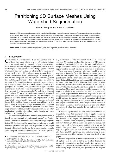
308 IEEE TRANSACTIONS ON VISUALIZATION AND COMPUTER GRAPHICS, VOL. 5, NO. 4, OCTOBER-DECEMBER 1999 

Partitioning 3D Surface Meshes Using 

Watershed Segmentation 

Alan P. Mangan and Ross T. Whitaker 

AbstractÐThis paper describes a method for partitioning 3D surface meshes into useful segments. The proposed method generalizes 

morphological watersheds, an image segmentation technique, to 3D surfaces. This surface segmentation uses the total curvature of 

the surface as an indication of region boundaries. The surface is segmented into patches, where each patch has a relatively consistent 

curvature throughout, and is bounded by areas of higher, or drastically different, curvature. This algorithm has applications for a variety 

of important problems in visualization and geometrical modeling including 3D feature extraction, mesh reduction, texture mapping 3D 

surfaces, and computer aided design. 

Index TermsÐSurfaces, surface segmentation, watershed algorithm, curvature-based methods. 

æ 

1 INTRODUCTION 

CONSIDER a 3D surface mesh. It can be described as a set 

of faces that share edges, or a set of vertices that are 

connected to neighboring vertices by edges. In many cases, 

such meshes have no explicit higher-level structure; they 

exist simply as a collection of connected polygonsÐa bucket 

of polygons. One way to impose a higher level structure on 

such a mesh is to partition it into a set of connected pieces, 

which themselves have relationships to other pieces. 

Presumably, the pieces should represent something about 

the underlying structure of the object itselfÐthe semantic 

meaning of the object's parts and subparts. However, when 

no structure, other than the local connectedness of the 

polygons, is specified, any algorithm seeking to partition 

such meshes must infer some structure from the local shape 

(e.g., geometry) of the mesh itself. We call the problem of 

partitioning a 3D surface mesh into meaningful, connected 

pieces the mesh segmentation problem. By meaningful, we 

propose that the relative size and organization of the 

segmented regions must be relevant to the application at 

hand. This problem bears a strong resemblance to the 

partitioning of images in image processing and computer 

vision. The mesh segmentation problem, like the image 

segmentation problem, is not well posed; solutions are often 

application specific, depending quite heavily on one's 

definition of ªmeaningful.º 

The 3D mesh segmentation method we present here is 

based on the concept of ªcatchment basinsº or ªwatersheds,º 

which has been used previously in image segmentation 

[1]. For images, the algorithm operates on a height 

function (usually the gradient magnitude of the input 

image), which is defined over the image domain, typically 

some compact, continuous subset of < 2 . This work presents 

. A.P. Mangan is with Creare Inc., PO Box 71, Hanover, NH 03755. 

E-mail: spm@creare.com. 

. R.T. Whitaker is with the Department of Electrical Engineering, 

University of Tennessee, Knoxvill, TN 37996-2100. 

E-mail: rtw@utk.edu. 

For information on obtaining reprints of this article, please send e-mail to: 

tvcg@computer.org, and reference IEEECS Log Number 109330. 

a generaliztion of the watershed method in order to 

segment 3D surface meshes. For the case of 3D meshes, 

the height function is defined over the mesh itself. One such 

height function is the total curvature of the surface (or some 

approximation thereof) defined at each vertex of the mesh. 

There are several reasons why one would want to 

segment a 3D mesh. Generally, datasets are more manageable 

at the higher level of abstraction that such a 

partitioning affords. There are also some specific applications 

that could benefit from such a capability. One example 

is mesh reduction [2], [3]. Effective mesh reduction algorithms 

can dramatically reduce the amount of data in a 3D 

mesh while maintaining, to a certain degree, the fidelity of 

the surface. Most mesh reduction algorithms operate on the 

data as a whole, with individual vertices or faces treated 

solely with respect to their immediate neighbors. However, 

we propose mesh segmentation as a preprocessing step that 

could indicate to subsequent mesh reduction algorithms 

that they should preserve distinct parts of objects. Results in 

this paper will show that a mesh segmentation technique 

that relies on surface curvature can help preserve edges, 

creases, and other fine details during subsequent mesh 

reduction. 

A related application is the reparameterization of 

irregularly connected meshes in order to apply successive 

reduction or refinement algorithms. For instance, Lee et al. 

[4] describe a technique that generates a hierarchy of 

regular meshes from irregularly connected meshes of 

arbitrary topology. This process can preserve designated 

vertices and edges that are important to the structure of the 

object. The generation of such special structures could 

require a great deal of user input. Alternatively, those 

structures could be generated automatically using a mesh 

segmentation algorithm such as the one described in this 

paper. 

Another application of mesh segmentation is the fitting 

of higher-order models to polygonal meshes. Because the 

proposed segmentation method breaks the surface into 

regions comprised of relatively consistent curvature (and 

bounded by high curvature), the geometry of the regions 

1077-2626/99/$10.00 ß 1999 IEEE

MANGAN AND WHITAKER: PARTITIONING 3D SURFACE MESHES USING WATERSHED SEGMENTATION 309 

tends to be homogeneous. Rather than using mesh reduction 

to decrease the complexity of the surface data, largescale 

structures, such as planes, quadrics, superquadrics, or 

B-splines, can be used to model these areas. For example, 

indoor scenes, or those consisting primarily of artificial 

objects, tend to have more planar and angular surfaces than 

those occurring in nature. In such cases, a higher-level 

modeling scheme consisting of geometric primitives might 

be appropriate. Outdoor scenes, on the other hand, are 

typically less organized and might be better modeled using 

algebraic structures or B-splines. Each region of the surface, 

having been segmented and classified according to surface 

type, could have a model assigned to it. 

A further use of mesh partitioning is the modification of 

existing 3D CAD models. As 3D models become more 

ubiquitous and available from a large number of difference 

sources (e.g., through the internet), interesting models tend 

to be in formats that are inappropriate for certain applications. 

In such cases, people using these models will be 

interested in modifying them to suit their own needs. Using 

the proposed surface segmentation scheme, a user could 

impose some structure on such models (perhaps after scan 

converting or tiling them). The model can then be modified 

on a region-by-region basis, making it easier to concentrate 

on a specific portion of the design. Sections and subassemblies 

of the model can be isolated for modification. Portions 

of structures in this manner could also be imported from 

existing parts databases and reused. 

Another application of mesh segmentation is feature 

detection. In some applications, such as medical imaging, 

one would like to locate points or lines on a surface that 

could serve as landmarks for comparing or aligning it with 

other surfaces. These landmarks should be relatively 

insensitive to noise and invariant to certain kinds of 

geometric transformations. One way to establish a set of 

landmarks is to use the boundaries of segments, particularly 

when those boundaries have some geometric interpretation, 

as is the case with the methods proposed in this 

paper. 

The remainder of the paper proceeds as follows: The next 

section describes some aspects of the literature that are 

related to the proposed algorithm. Section 3 presents the 

watershed algorithm in the context of images and then the 

generalization to 3D meshes. After completion of the 

watershed segmentation, it is also necessary to perform an 

additional step of region merging in order to avoid oversegmentation, 

that is, to control the level of detail in the 

segmentation. That section also describes the region 

merging process and Section 4 explains how surface 

curvature is computed, both directly from isosurfaces of 

volumes and from vertex-list type geometric models. 

Section 5 presents results and analyzes the performance of 

the algorithm. It describes the capability of the algorithm to 

segment simple surfaces, the effects of added noise, and the 

performance of the algorithm when segmenting complex 

surfaces. 

2 RELATED WORK 

There are several somewhat diverse areas of research that 

are relevant to this work. One area is the problem in 

computational geometry of attempting to divide polyhedra 

into convex components. Another area is the 

detection of geometric features, namely creases, on 

continuous surfaces. Another related area is the problem 

of surface classification from range data. Last, there is 

that part of image processing which applies morphological 

watersheds to image segmentation. 

In the field of computational geometry, researchers [5], 

[6] have addressed the problem of dividing polyhedra into 

collections of convex pieces. Of course, the individual faces 

are each convex, but if one considers the optimal partitioning 

(e.g., smallest number of pieces), the problem is NPcomplete 

[7]. Several researchers have proposed reasonable 

algorithms for obtaining good solutions. Unlike the problem 

addressed in this paper, the convex-decomposition problem 

is purely geometric and is well posed; state-of-the-art 

research focuses on developing efficient algorithms. Such 

a convex decomposition is useful for algorithms that 

explicitly depend on convex objects (such as certain 3D 

rendering algorithms or collision detection), but less useful 

for applications that are trying to get a part-subpart 

decomposition that is related to the underlying structure 

of the object. For instance, a convex decomposition must 

partition hyperbolic regions into their constituent flat 

facesÐa partitioning which has little to do with the overall 

shape of an object (e.g., a torus) that happens to contain 

such regions. Fig. 1a shows an example of how two objects 

joined by a smooth fillet create a hyperbolic region. In this 

example, a convex decomposition will produce less than 

adequate results (Fig. 1b) and will, without heuristics, 

partition the hyperbolic region into its constituent (atomic) 

planar faces. In this same example, a curvature-based 

segmentation could, in principle, partition the surface along 

meaningful, intuitive boundaries (e.g., Fig. 1c) that divide 

the faces of objects and break the protrusion from the main 

body of the larger object. 

Another related problem is the detection of certain kinds 

of geometric features on surfaces. The detection of such 

features can be important in comparing, registering, and 

analyzing shapes. Perhaps the most closely related idea is 

ªridge detectionº on surfaces [8], [9]. Because ridges are 

usually assumed to be maxima in curvature, the operators 

required to detect them rely upon third- and fourth-order 

derivatives. Such derivatives are very sensitive to noise, 

requiring some robust approximation, such as a polynomial 

fit or a low-pass filterÐboth of which tend to distort the 

shapes of the features being detected. For this reason, there 

are few examples in the literature that make practical use of 

such surface ridges for segmenting 3D meshes. Our method 

does not attempt to explicitly locate ridges. Rather, the 

surface is segmented into patches bounded by regions where 

sharp differences in surface normal create a boundary. 

Although these boundaries do occur at places of high 

curvature, the watershed algorithm makes no attempt to 

explicitly locate these edges/ridges and does not require 

derivatives beyond second-order (first-order derivatives of 

the normal). 

Surface segmentation is also related to the problem of 

surface classification. Extracting surface patches by identifying 

individual surface elements as certain types has played


Fig. 1. Convex decomposition. (a) A protusion is joined to a larger object by a smooth fillet, creating a hyperbolic region. (b) A convex decomposition 

divides the surface along lines that are not perceptually meaningful while decomposing the hyperbolic region into its constituent planar faces. (c) A 

curvature-based method could, in principle, partition the surface along lines that distinguish individual faces and part/subpart boundaries. 

an important role in high-order systems, such as 3D 

recognition. For instance, Fisher et al. [10] address the 

problem of extracting surface patches from range data with 

the goal of constructing CAD models. Their method uses a 

curvature-based surface classification algorithm to perform 

segmentation. Faugeras and Hebert [11] also approach the 

problem of 3D segmentation from a scene recognition 

viewpoint. They perform geometric matching between 

primitive surfaces (mainly planar, although the more 

general case of quadrics is discussed). Besl [12] proposes 

using the mean and Gaussian curvatures in segmenting and 

classifying surfaces by type. These approaches are based on 

range data, which is always a graphÐa special class of 3D 

surfacesÐwhereas the method we propose is suited to the 

more general class of 3D surfaces. We make use of the mean 

and Gaussian curvatures in calculating the total curvature, 

but do not explicitly attempt to classify any particular 

surface region. Rather than use only local differential 

structure to classify regions into one of several simple 

types, we partition regions based on the homogeneity of the 

surface normal, combining local information at many points 

to form a region. Thus, the proposed algorithm is broadly 

applicable to many types of 3D surfaces and does not rely 

upon the classification and matching of any type of 

underlying geometric primitive. 

Similarly, the computer vision literature shows examples 

of the application of image segmentation techniques to 

surfaces, such as range maps, that are height functions, i.e., 

z ˆ f…x; y†, defined on a rectilinear grid [13], [14]. These are 

essentially image segmentation techniques that include 

some analysis of the local image surface structure. The goal 

of this paper is to describe the generalization of one such 

algorithm to a full 3D surface and demonstrate its 

effectiveness in addressing several problems in computer 

graphics and vision. 

The problem of segmentation is central to image 

processing and computer vision and has been an area of 

active research for more than 30 years. Watersheds for 

image segmentation are described in the classic work of 

Serra [1] on mathematical morphology. Since that time, they 

have found a wide range of applications including medical 

imaging [15], [16], shape analysis [17], and range-image 

segmentation [14]. KoeÈnderink and Van Doorn [18] argue 

for watersheds as a method of detecting ªridgesº as an 

alternative to constructing detectors that rely on higherorder 

derivatives. Eberly [9] gives a nice overview of that


Fig. 2. Watershed strategies. (a) The bottom-up approach to finding catchment basins is to start at a local minimum and incrementally flood the 

region until it connect to its neighbors. (b) The top-down approach is to place a token at a point and move the token along a steepest descent until it 

reaches a minimum. 

debate and also discusses the use of scalar functions defined 

on manifolds as a means of detecting ridges. 

In this paper, we use the notion of defining a scalar 

function on a manifold (in this case, the scalar function is 

surface curvature and the manifold is a 3D surface mesh), 

but we apply morphological watersheds as a means of 

segmenting that surface. The algorithm we use traces points 

on the surface ªdownº to local minima, as in [15]. The 

difference with the proposed algorithm and previous work 

is the generalization of morphological watersheds to a 3D 

polygonal mesh and the use of a depth measure to reduce 

insignificant regions. 

3 WATERSHED ALGORITHM 

This section describes the strategy used in the watershed 

algorithm and the specifics of the implementation. The 

image processing version of the algorithm is first briefly 

introduced and an example of image segmentation using 

this approach is given. The generalization of the algorithm 

from a 2D rectilinear grid to an arbitrary surface with welldefined 

neighbor connectivity is then presented. 

3.1 Watersheds in Image Processing 

The watershed algorithm derives its name from the manner 

in which regions are segmented into catchment basins. Let 

f…x; y† : U !< be a continuous height function defined 

over the image domain U < 2 . A catchment basin is the set 

of points whose path of steepest descent terminates in the 

same local minimum of f. The choice of height function 

depends on the application; the basic algorithm is independent 

of the height function. For instance, one might choose 

the original image in order to locate blobs (light and dark 

regions), as in [15], or one could choose the gradient 

magnitude of the image in order to locate regions that are 

relatively homogeneous [14]. 

After locating these minima in f, there are two strategies 

for associating catchment basins with these minima. One 

strategy is to incrementally ªfloodº the regions surrounding 

these minima, keeping track of the places where flood 

regions touch [1], [14]. This method typically requires one to 

discretize the range (or gray levels) of f, thus limiting the 

contrast resolution of the resulting segmentation. If the 

domain of f is discrete (as is usually the case), an alternative 

is to take each point in U and flow downward until one 

encounters a minimum or a point which has already been 

associated with a minimum (see Fig. 2). The connectivity of 

the points in U depends on the discretization, but, with 

rectilinear grids, four connectivity is usually sufficient. If 

labels are updated incrementally, the computation time is 

proportional to the number of points in the image times the 

connectivity. For 3D mesh segmentation, we have chosen 

the latter approach, which we call the top-down approach, 

because it is better suited for the irregular topology of the 

3D mesh. In both algorithms, there are special cases that 

must be considered. For instance, there may be flat regions, 

plateaus, where there is no downhill direction across 

neighboring vertices. Such details are discussed in the 

sections that follow. 

An example of the application of the watershed algorithm 

to images serves as a good starting point for the 

extension to 3D meshes. Fig. 13 shows an input image, the 

gradient magnitude of that image (which serves as f), and 

the segmentation that results from following pixels (using 

four-connected neighbors) through a steepest descent to the 

local minima. 

3.2 Extension to 3D 

Our goal is to extend this algorithm to a 3D mesh consisting 

of connected vertices, each of which has a value of f and a 

set of connections to neighboring vertices, as displayed in 

Fig. 3. Let X be the set of all vertices in the mesh. For each 

x i X, there is a connected neighborhood of x i , N i X. 

Such a neighborhood is shown in Fig. 3. In the image 

processing case, we traverse a 2D network of points where 

each point's neighbors are defined by a rectilinear grid. In 

the case of a surface mesh, we move tokens around a 

network of points in 3D, where each point's neighbors vary, 

depending upon the mesh geometry and connectivity at 

that point. A token moves from one vertex to its neighbor of


Fig. 3. Neighborhood relationships for a 2D rectilinear grid (left) and a 3D mesh of connected vertices (right). 

lowest value until it reaches a minimum (which it must, by 

definition). The 3D positions of the vertices are not relevant 

to this process; only the topology of the vertices and the 

values of the height function affect the formation of 

catchment basins. Thus, the shape of the surface affects 

the segmentation via the height function. 

Therefore, the steps of the watershed segmentation 

algorithm are as follows: 

1. Compute the curvature (or some other height 

function) at each vertex. 

2. Find the local minima and assign each a unique 

label. 

3. Find each flat area and classify it as a minimum or a 

plateau. 

4. Loop through plateaus and allow each one to 

descend until a labeled region is encountered. 

5. Allow all remaining unlabeled vertices to similarly 

descend and join to labeled regions. 

6. Merge regions whose watershed depth is below a 

preset threshold. 

The following sections describe in more detail the 

specific steps for computing the watershed segmentation. 

The input to the watershed method is a surface mesh and 

whatever additional information (e.g., surface normals) is 

necessary to calculate the curvature at each vertex. The 

algorithm then segments this mesh, using the curvature as 

the height function f. Thus, the first step of the segmentation 

is the calculation of curvature at each vertex on the 

surface. The method for calculating curvature should 

depend on the application and type of input data available. 

The methods for curvature calculation used in this work are 

discussed in Section 4. The watershed algorithm, per se, is 

independent of the type of curvature used. 

3.3 Initial Labeling 

Once the curvature (height function) is defined on the 

surface mesh, the watershed method labels all of the local 

minima, i.e., those vertices with curvature lower than that 

of all of their neighbors, as in Fig. 4a. Each minimum then 

serves as the initial basis for a surface segment, i.e., a 

distinct region on the surface formed during the descent of 

vertices along their paths of steepest descent. Next, flat 

regions are found. These are one of two types as shown in 

Fig. 4b; either flat plateaus or flat minima. Flat plateaus are 

defined as those flat regions that have any vertices adjacent 

to their borders with a lower curvature than that of the 

plateau itself. A variation of the algorithm is to define an 

additional type of flat region; the flat maximum, which has 

all adjacent points lower than itself. These maxima may also 

be used as indicators of borders between regions. We treat 

these maxima, if present, in the same manner as flat 

plateaus and do not explicitly define any points as border 

vertices. Flat minima have all adjacent vertices with higher 

curvatures than themselves. These minima are labeled and 

treated in the same manner as local single-vertex minima. 

Once all flat regions are found and classified, a descent is 

made from each of the flat plateaus until a labeled region is 

encountered. The curvatures of all adjacent vertices of the 

plateau are examined and the descent from the plateau 

begins at that vertex with the lowest curvature. 

3.4 Descent 

The process of associating points together into catchment 

basins is what gives this method the name ªwatershed.º 

Imagine a drop of water placed at the starting vertex, 

flowing downhill on the height function, i.e., toward the 

point of lowest curvature. The drop, or token, follows the 

path of gradient descent, and each vertex it encounters on 

its path ªdownwardº is labeled with the same identifying 

label as the first labeled vertex it encounters, as shown in 

Fig. 2b. This token moves all of the way to a local (labeled) 

minimum or hits a labeled vertex that has already been 

associated with a minimum. Initially, descent is made from 

flat plateaus, followed by the remaining unlabeled vertices 

on the surface. The plateau and its path of descent are then 

labeled and joined to the region finally hit during the 

descent. If another flat plateau is encountered, then the two 

are joined and the resulting plateau will later descend in 

turn until a minimum is encountered. The plateaus are 

indexed, and joined as necessary, so that a token, upon 

reaching a plateau, can move through it in one step and 

continue its descent. The next step is to allow all other 

unlabeled vertices to similarly descend until they hit a 

labeled region, then label them and join them to that region. 

3.5 Region Merging 

The final step of labeling each vertex according to its 

associated minimum produces a segmented mesh. However, 

the watershed, as it stands, is sensitive to even the


Fig. 4. Initial labeling. (a) Labeling of local minima and (b) classification of flat regions. 

smallest fluctuations in surface shapeÐevery local minimum 

of curvature establishes its own region. Leaving the 

surface in this state can yield a solution with regions that 

are too small and numerous to be useful (as shown in 

Fig. 10). It is necessary to merge the regions together in 

order to obtain reasonable results. The strategy is to use a 

saliency measure and the structure of the catchment basins 

to define a merging process. 

There are a variety of possibilities for metrics that 

indicate insignificant regions, but the watershed algorithm 

itself gives a fairly reliable metric for determining the 

saliency of a segment. This metric is the greatest depth of 

water that a segment can hold before it ªspills overº into 

one of its neighbors. Regions that are ªshallowº are 

relatively constant in curvature, i.e., their boundaries have 

a curvature which is not significantly greater than the 

flattest part of that region. The watershed depth can be 

calculated as the difference between the point in the region 

with the overall lowest curvature (the local minimum) and 

the vertex along the region's boundary with the lowest 

curvature of all other boundary vertices, as in Fig. 5. This is 

the depth of water that the region can hold before it begins 

to overflow its boundary. 

In calculating the lowest boundary point of a segment, it 

may be necessary to take into account those vertices 

immediately past the current region's boundary. This is a 

side effect of the discrete nature of the grid; because the 

watershed algorithm labels all vertices as being in one 

region or another, even though segments are separated by a 

single ridge of vertices which have downhill neighbors that 

flow into two separate catchment basins. These ridge 

vertices determine the minimum watershed depth. Notice 

that, in Fig. 5, the depth is found using such a vertex, vertex 

A. If the depth had merely been calculated using the vertex 

with the lowest curvature belonging to the current region, 

then vertex B would have been used, resulting in an 

incorrect, lower depth. 

The region merging algorithm is as follows: 

1. For each region, find its lowest point, neighbors, and 

lowest boundary point with each neighbor. 

2. Find depth of region, the difference between the 

lowest point to lowest boundary point. 

3. If depth is below a predefined threshold, merge this 

region to region adjacent to lowest boundary point 

and update new region's information accordingly. 

4. Repeat until no regions exist that are below the 

minimum depth. 

Once the depths of all regions are computed, those 

regions below the depth threshold are merged with their 

neighbors. In this manner, adjacent regions, at least one of 

which has a shallow depth, as in Fig. 6, are combined 

together. This drives the solution away from being oversegmented 

toward a more useful result. This merging 

process can be done very efficiently using the appropriate 

data structures and keeping a lookup table of merged 

regions. Several pieces of information must be tabulated for 

each region. The vertex with the lowest curvature for the 

region is found and used to later estimate the depth of the 

region. The boundary of the region is found and, from this, 

all neighboring regions are determined. For each neighbor 

B, the boundary vertex of the current region A adjacent to B 

with the lowest curvature is also found. From these 

boundary vertices, the lowest (in terms of curvature) 

boundary vertex of the region is then calculated. With this 

information, available region merging can then proceed. 

When a shallow region is identified, the neighboring 

region into which the lowest boundary vertex would flow 

during descent is selected as that one with which to merge. 

This resolves any ambiguity that might arise in the case of 

there being more than one neighboring region adjacent to 

the lowest boundary vertex. For implementation purposes,


Fig. 5. Defining the depth of a region based on its lowest vertex and lowest boundary vertex. 

rather than relabeling all of the region's vertices with the 

label of the neighboring region it just merged with, a 

pointer is set for the region indicating with which region it 

is merged. The pointers of all other regions merged with 

this one are also updated to reflect the new region with 

which they are now merged. 

When merging regions, one must also update the 

information of the new region regarding lowest vertex, 

lowest boundary vertex, and neighbors. Comparing and 

changing the lowest curvature vertex is straightforward; 

adjusting the neighbor information of this new region is 

somewhat more complicated. All of the current region's 

neighbors need to be added as neighbors of the new region 

unless they themselves have been merged with the new 

region previously. The current region, and all other regions 

in turn merged with it, are then removed from the new 

region's list of neighbors. The boundary vertices associated 

with these neighbors also are removed from their respective 

lists. The new lowest boundary vertex is next recalculated, 

necessary in case the region associated with the previous 

lowest boundary vertex. The regions are merged in this 

manner according to Fig. 7. Once this information is 

updated, the new lowest boundary vertex has to be 

calculated and set. This merging procedure is repeated, 

cycling through all of the regions consecutively until no 

Fig. 6. Merging adjacent regions with shallow depths. 

further regions are within the preset depth threshold. At 

this point, the watershed algorithm is complete. 

This basic strategy can be extended to incorporate other 

measures of saliency. Another natural measure is to 

compute the volume of the watershed (i.e., average depth 

times area), which would favor larger regions over smaller 

ones. One could also bring other information into this 

metric, such as triangle coloring or texture coordinates. We 

have experimented with area-based metrics and found that 

they penalize small areas too aggressively, which produces 

inferior results for the examples we have considered. The 

development, implementation, and verification of other 

saliency measures is an area for future work. 

4 CURVATURE CALCULATION 

The calculation of curvature depends on the type of data 

used and the level of noise in that data. In this work, we 

consider two different types of input: volumes whose 

voxels represent the value of some implicit function and 

simple surface meshes consisting of only vertices and 

triangles. In the former case, we can use the volume data 

itself to directly compute accurate estimates of the 

curvature of the embedded surface. Given a polygonal 

mesh (without an embedding) as input, there are several 

possibilities for discrete approximations to surface curvature. 

One approximation is the angle between the faces that 

are adjacent to a vertex. Another option is the norm of the 

covariance of the surface normals or edges that are adjacent 

to that vertex. 

4.1 Isosurface Curvature 

In the case of volumes, we are segmenting meshes 

corresponding to isosurfaces. The meshes are generated 

using the marching cubes algorithm [19]. Therefore, we 

can compute the curvature of the isosurface using the 

values of the volume itself as the surface is extracted. 

This provides a slightly more accurate estimate of the 

surface curvature than that obtained using the faces that


Fig. 8. Thresholding the total curvature. 

Fig. 7. Region merging. As each new region is added to the current 

region, indicated by the shaded area, its list of neighbors and associated 

boundary vertices needs to be updated accordingly. 

are generated from the marching cubes algorithm. For the 

magnitude of the curvature, we use the deviation from 

flatness [20], which is defined to be the Euclidean norm of 

the shape tensor. The mean, H, and Gaussian 

curvature,K, are first found from [21], 

 

2 x … yy ‡ zz †‡ 2 y … 

xx ‡ zz † 

‡ 2 z 

H ˆ 

… xx ‡ yy †2 x y xy 2 z x xz 2 y z yz 

… 2 x ‡ 2 y ‡ 2 z †3=2 

K ˆ 

0 

2 x … yy zz yz yz †‡ 2 y … 1 

xx zz xz xz † 

@ ‡ 2 z … xx yy xy xy †‡2… x y … xz yz xy zz † A 

‡ y z … xy xz yz xx †‡ z x … xy yz xz yy †† 

… 2 x ‡ 2 y ‡ ; 

2 z †2 

where represents the value of the implicit function at a 

given point in the volume. The total curvature, D, is then 

calculated using: 

p 

D ˆ 

 

4H 2 2K 2 : …3† 

When computing the curvature values, we sometimes 

apply a threshold to the curvature, as shown in Fig. 8. This 

step is performed so that relatively flat areas where the 

curvature is extremely low throughout will be classified as 

exactly flat, easing the computational burden during later 

processing. This threshold does not have a significant affect 

on the final result because such shallow watersheds would 

be merged in the last part of our algorithm, as discussed in 

Section 3.5. Once this threshold has been applied, the 

watershed algorithm proper can begin. 

4.2 Surface Mesh Curvature 

There are several possibilities for finding the curvature of 

surfaces represented by polygonal meshes. We have 

…1† 

…2† 

experimented with two different approaches and achieved 

varying degrees of success for each. The first method uses 

the angles between the faces of the triangles to determine 

the curvature. The second uses the norm of the covariance 

of the surface normals adjacent to the vertex in question. 

The latter method proved to be the most successful because 

it is less sensitive to noise and it averages across faces that 

are composed simply of pairs of coplanar triangles. 

To find the covariance matrix, the variance and covariance 

in all three cardinal directions must first be found. The 

variance and covariance are found from: 

2 aa ˆ 1 X N 

…a t a† 2 

…4† 

N 

tˆ0 

2 ab ˆ 1 X N 

…a t a†…b t b† 

N 

tˆ0 

…5† 

a 2fx; y; zg b 2fx; y; zg: …6† 

N represents the number of triangles associated with this 

vertex and ‰x t y t z t Š are the components of the normal for 

triangle t. Also, ab ˆ ba . The curvature, D, is then set equal 

to the norm of the covariance matrix, C; 

2 

xx xy 

3 

xz 

D ˆkCk C ˆ 4 yx yy yz 

5: …7† 

zx zy zz 

4.3 Edge-Node Meshes 

If the input to the algorithm is a triangle (or polygonal) 

mesh rather than a volume, one must also consider the 

segmentation relative to the underlying structure of the 

mesh. So far we have assumed that we are dealing with a 

mesh created from a volume and that the mesh is ªdense,º 

i.e., there are many vertices for each surface region. The 

watershed algorithm operates on connected nodes in this 

mesh. However, for tessellated surfaces, the model is 

frequently sparse, with just enough vertices to define each 

surface (particularly a problem in planar areas), and some 

large regions might not contain enough vertices to define a 

catchment basin with an associated boundary. 

This problem can be solved by creating a new mesh, the 

dual of the original, which has a node for each edge in the 

original mesh and a connection to each adjacent edge (now 

nodes) across the faces of the two neighboring triangles (or 

polygons). This shifts the emphasis of the algorithm from 

the vertices to the polygons of the mesh. For each edge, i.e., 

between every pair of vertices, in the original mesh, there is 

a corresponding node in the new mesh. The curvature of 

this node is then set as the average of its neighboring 

vertices' curvatures. After region merging is performed,


curvature) at each node, a variety of different approximations 

and preprocessing algorithms can be applied to both 

the mesh itself and the height function. For instance, an 

iterative smoothing process could be applied to the height 

function in order to reduce the effects of noise and 

approximation errors. Such preprocessing is an area of 

ongoing investigation and is beyond the scope of this paper. 

Fig. 9. Creation of edge-based topology based on original mesh. 

triangle regions are established, with each triangle being 

evaluated for region membership based on whether all 

three of its edges belong to the region in question. 

Because the watershed algorithm is independent of how 

one structures the mesh or computes the height function (or 

5 RESULTS 

In this section, we present the results of using the watershed 

algorithm to perform segmentation of surface meshes. We 

show initial results obtained prior to region merging; 

examination of these oversegmented solutions demonstrates 

the need for region merging. The algorithm's 

capability to successfully segment simple geometric shapes 

is demonstrated. The performance of the algorithm in the 

presence of noise is analyzed. The sensitivity of the 

segmentation to the user-defined threshold is shown. 

Segmentation results for the edge-node meshes, described 

in Section 4.3, are then given. Finally, some examples of 

applications that benefit from the use of this segmentation 

technique are given, such as mesh reduction and region 

extraction for CAD models. 

Fig. 10. Oversegmentation resulting from not applying the final region merging step of the algorithm.


Fig. 11. Segmentation of various test surface types. (a) Cube (six regions), (b) cylinder (three regions), (c) sphere (one region), and (d) torus (two 

regions). 

5.1 Oversegmentation 

This section demonstrates the need for region merging by 

displaying some results obtained without performing the 

final merging step. As is seen in Fig. 10, the output of the 

watershed algorithm suffers quite badly from oversegmentation. 

Any small defects or noise present in the initial 

model allow the formation of bumps on the surface. If these 

bumps are concave, they in turn lead to the creation of local 

minima, which become isolated regions as neighboring 

vertices flow into them. 

5.2 Segmentation of Simple Surfaces 

Fig. 11 shows the segmentation results for several analytically 

defined surfaces with known curvature characteristics. 

Fig. 11a shows the segmentation of a cube (extracted from a 

volume), the six faces of which are planar, each separated 

by a ªwallº of high curvature. The high curvature at the 

edges of the cube allows the algorithm to decompose the 

surface into the six regions as shown. A similar boundary of 

high curvature separates the two planar areas at the ends of 

the cylinder in Fig. 11b. The sphere also has a consistent 

degree of curvature throughout its surface and is segmented 

into a single region in Fig. 11c. The torus in Fig. 11d has 

varying curvature and surface type (it is hyperbolic on the 

inner hull and elliptic on its outer hull). The curvature also 

has a pair of maximal loci around the inner and outer hulls 

that have created the boundary between the two regions as 

displayed. 

5.3 Noise Analysis 

This section examines the performance of the algorithm in 

the presence of additive, uniform noise. For the following 

analyses, uniform noise is added to the curvature of the 

vertices as a percentage of the range of curvature for the 

object, D vertex ˆ D vertex …X% of…D max D min ††. Fig. 12 

shows how noise affects the segmentations of a torus and 

a cube. The torus has a relatively constant level of curvature 

on its surface, whereas the cube has, in effect, zero 

curvature except at the boundaries between faces. Fig. 12a, 

Fig. 12b, and Fig. 12c show the torus with varying levels of 

additive noise applied to the curvature of each vertex. For 

small levels of noise, 2.5 percent to 5 percent, the boundary 

between regions moves, but the torus is still segmented into 

two regions, as appropriate. However, as the noise reaches 

10 percent, the partitioning fails dramatically and the torus 

is oversegmented into 36 regions. At this noise level, the 

segmentation no longer corresponds to the underlying 

geometry of the torus. The cube, Fig. 12d, Fig. 12e, and Fig. 

12f, displays less sensitivity to small levels of noise. Adding 

small levels of noise to the boundaries separating the planar 

faces has negligible effect. As with the torus, once the noise 

reaches a sufficiently high level, 10 percent, the boundary 

curvature is no longer significantly higher than the faces 

and the segmentation breaks down. 

5.4 Threshold Sensitivity 

The algorithm displays sensitivity to the user-specified 

threshold encountered in the region merging step. Varying 

the threshold allows for different levels of segmentation, the


of view [22]. Because this data is from a sensor, it shows 

some level of noise. A comparison of results of segmentations 

using different threshold levels shows that increasing 

the threshold leads to fewer final regions, as those with 

successively lower depths are merged with neighboring 

regions. The boundaries between regions in Fig. 14a 

represent edges and breaks that are not as highly curved 

as those in Fig. 14d. There are several areas of interest in the 

scene that are initially segmented into several pieces, but, as 

the threshold increases, they are gradually segmented into 

fewer, more coherent regions. Note how the floor is at first 

partitioned into multiple areas. The wall partitions, barrels, 

chairs, and printers (on the lefthand side of the scene) are 

also partitioned into successively fewer regions. 

Fig. 15 shows the segmentation of a dart object, again 

with several threshold levels. The surface in this case is 

much simpler than that shown in Fig. 14, yet also displays 

the same characteristics as the threshold varies. 

5.5 Segmentation Based on Mesh Input 

All of the segmentation examples thus far have been created 

using curvature calculated from volumetric inputs as 

discussed in Section 4.1. Here, we present a segmentation 

based on surface-based curvature, as described in Section 

4.2. The input to the system in this case is a surface mesh 

rather than a volume. Fig. 16 shows two segmentations of 

the mug model using different thresholds. This method is 

capable of generating useful results, but appears to be more 

prone to high frequency artifacts than segmentations 

produced from volumetric input. It is possible that these 

effects could be overcome by applying some type of lowpass 

filter to the curvature data; we have chosen here to 

concentrate on the segmentation aspects of the problem and 

leave this extension of the work for future completion. 

Fig. 12. Torus and cube segmentations with different levels of additive 

noise applied. (a) Torus, 2.5 percent noise (two regions), (b) torus, 5 

percent noise (two regions), (c) torus, 10 percent noise (36 regions), (d) 

cube, 2.5 percent noise (six regions), (e) cube, 5 percent noise (six 

regions), (f) cube, 10 percent noise (43 regions). 

exact level depending upon the final application. Fig. 14 

shows segmentation results for a 3D model of a room that 

was built by fusing laser range images from different points 

5.6 Applications 

As mentioned previously, there are several areas that can 

benefit from this segmentation technique. The advantages 

of using surface segmentation in two of these areas, mesh 

reduction and CAD, are highlighted here. 

One of the possible applications of the proposed surface 

segmentation method is improving the results of mesh 

reduction algorithms. In Fig. 18, we show the results of 

applying mesh reduction to the dart for various reduction 

rates. We use an iterative edge-collapse decimation strategy 

[2], which incorporates a greedy algorithm operating on a 

Fig. 13. Example of image segmentation using the watershed algorithm. (a) Input image, (b) gradient magnitude of the input image, smoothed with a 

Gaussian filter, (c) segmentation of (b) using the watershed algorithm.


Fig. 14. Segmentation of a scene using varying thresholds, indicated by T. (a) T ˆ 0:275 (957 regions), (b) T ˆ 0:4 (498 regions), (c) T ˆ 0:425 (441 

regions), (d) T ˆ 0:455 (381 regions). 

Fig. 15. Dart segmentations. (a) T ˆ 0:15 (103 regions), (b) T ˆ 0:2 (64 regions), (c) T ˆ 0:4 (36 regions). 

Fig. 16. Segmentation of the mug model using surface-based curvature calculations. (a) T ˆ 0:05 (42 regions), (b) T ˆ 0:0025 (126 regions). 

curvature metric [23], [24]. Fig. 18a and Fig. 18b show the 

results of reduction by factors of 50 and 100 respectively. 

Fig. 18c and Fig. 18d display the improvement possible by 

specifying the same reduction rates on this surface after it 

has been segmented. In the latter case, reduction was not 

allowed across region boundaries, preventing edges between 

vertices in different regions from collapsing into a


Fig. 17. Several subassemblies of the dart model isolated via region extraction. 

single vertex. In this manner, the region boundaries (edges) 

are preserved. 

Another area that can benefit from the use of the 

segmentation method proposed here is that of computeraided 

design. It is possible to read in a general mesh model 

without any knowledge of its structure save its basic 

connectivity and segment it and extract any desired regions 

using the user-specified threshold. Subparts can then be 

analyzed in detail and the model modified by modifying or 

deleting assemblies as required. These parts and assemblies 

can then be added to a database of such parts and 

recombined and reused in different configurations as 

needed. A surface mesh can be created using an interactive 

3D model generation tool and measurements and specifications 

for various subassemblies then generated from the 

segmented model. Fig. 17 shows several parts of the dart 

extracted from the model as a whole. 

6 CONCLUSIONS 

We have presented here a method of surface segmentation 

which uses a generalization of watershed regions to 3D 

meshes. The method can segment either isosurfaces of a 3D 

volume or surface meshes directly into regions that are 

bounded by higher curvature. The algorithm displays some 

sensitivity to the user-specified threshold. Varying the 

threshold allows for different levels of segmentation, the 

exact level depending upon the final application. 

One aspect of the system that would benefit from future 

work is the method of calculating curvature for surface 

meshes. Currently, the results obtained from segmentation 

of these meshes are prone to high frequency aliasing and 

Fig. 18. Mesh reduction on unsegmented and segmented surface. (a) Reduction by a factor of 100 on the unsegmented dart, (b) the vertex 

connectivity of the unsegmented reduction, (c) reduction by a factor of 100 on the segmented dart, (d) the vertex connectivity of the segmented 

reduction.


the success of the segmentation depends heavily upon the 

coarseness of the grid sampling. Smoothing the curvature 

calculated from these surfaces will, in all probability, 

improve the segmentation results significantly. 

ACKNOWLEDGMENTS 

Thanks go to David Breen and the Computer Graphics 

Group at the California Institute of Technology for providing 

the dart volume data and to Chris Gourley for 

providing the mesh reduction code. The image segmentation 

example was provided by Samuel Burgiss Jr. The range 

data in Fig. 13a was provided by the Oak Ridge National 

Laboratory. This work is supported by the U.S. Office of 

Naval Research Visualization program under grant N00014- 

97-0227. 

REFERENCES 

[1] J.P. Serra, Image Analysis and Mathematical Morphology. London: 

Academic Press, 1982. 

[2] H. Hoppe, ªProgressive Meshes,º Computer Graphics (Proc. 

SIGGRAPH 96), pp. 99-108, July 1996. 

[3] A. Varshney, P. Agarwal, and F.P.B. Jr, ªAutomatic Generation of 

Multiresolution Hierarchies for Polygonal Models,º Proc. First 

Workshop Simulation and Interaction in Virtual Environments, pp. 25- 

28, 1995. 

[4] A.W.F. Lee, W. Sweldens, P. SchroÈder, L. Cowsar, and D. Dobkin, 

ªMAPS: Multiresolution Adaptive Parameterization of Surfaces,º 

Computer Graphics (Proc. SIGGRAPH 98), pp. 95-104, July 1998. 

[5] C.L. Bajaj and T.K. Dey, ªConvex Decompositions of Polyhedra 

and Robustness,º SIAM J. Computing, vol. 21, pp. 339-364, 1992. 

[6] B. Chazelle and L. Palios, ªTriangulating a Nonconvex Polytope,º 

Discrete and Computational Geometry, vol. 5, pp. 505-526, 1990. 

[7] B. Chazelle, D.P. Dobkin, N. Shouraboura, and A. Tal, ªStrategies 

for Polyhedral Surface Decomposition: An Experimental Study,º 

Proc. 11th Ann. ACM Symp. Computational Geometry, pp. 297-305, 

June 1995. 

[8] J. KoeÈnderink and A. van Doorn, ªThe Structure of Two- 

Dimensional Scalar Fields with Applications to Vision,º Biological 

Cybernetics, vol. 33, pp. 151-158, 1979. 

[9] D. Eberly, Ridges in Image and Data Analysis. Dordrecht: Kluwer 

Academic, 1996. 

[10] R.B. Fisher, A.W. Fitzgibbon, and D. Eggert, ªExtracting Surface 

Patches from Complete Range Descriptions,º Proc. Int'l Conf. 

Recent Advances in 3-D Digital Imaging and Modeling, pp. 148-154, 

Ottawa, Canada, May 1997. 

[11] D. Faugeras and M. Hebert, ªA 3-D Recognition and Positioning 

Algorithm Using Geometric Matching between Primitive Surfaces,º 

Proc. Eighth Int'l Joint Conf. Artificial Intelligence, pp. 996- 

1,002, 1983. 

[12] P. Besl, Surfaces in Range Image Understanding. Springer-Verlag, 

1988. 

[13] E. Trucco and R.B. Fisher, ªExperiments in Curvature-Based 

Segmentation of Range Data,º IEEE Trans. Pattern Analysis and 

Machine Intelligence, vol. 17, no. 2, pp. 177-182, Feb. 1995. 

[14] M. Baccar, ªSurface Characterization Using a Gaussian Weighted 

Least Squares Technique towards Segmentation of Range 

Images,º master's thesis, Univ. Tennessee, Knoxville, May 1994. 

[15] A.C.F. Colchester, ªNetwork Representation of 2D and 3D 

Images,º 3D Imaging in Medicine, K.H. HoÈhne, H. Fuchs, and 

S. Pizer, eds., pp. 45-62, Springer-Verlag, 1990. 

[16] L.D. Griffin, A.C.F. Colchester, and G.P. Robinson, ªScale and 

Segmentation of Gray-Level Images Using Maximum Gradient 

Paths,º Image and Vision Computing, vol. 10, pp. 389-402, 1992. 

[17] L.R. Nackerman, ªTwo-Dimensional Critical Point Configuration 

Graphs,º IEEE Trans. Pattern Analysis and Machine Intelligence, 

vol. 6, no. 4, pp. 442-450, 1984. 

[18] J. KoeÈnderink and A. van Doorn, ªLocal Features of Smooth 

Shapes: Ridges and Courses,º SPIE Proc. Geometric Methods in 

Computer Vision II, vol. 2031, pp. 2-13, 1993. 

[19] W.E. Lorensen and H.E. Cline, ªMarching Cubes: A High 

Resolution 3D Surface Construction Algorithm,º Computer Graphics 

(Proc. SIGGRAPH 87), vol. 21, pp. 163-169, July 1987. 

[20] J. KoeÈnderink, Solid Shape. Cambridge, Mass.: MIT Press, 1991. 

[21] J. Sethian, Level Set Methods: Evolving Interfaces in Geometry, Fluid 

Mechanics, Computer Vision and Materials Science. New York: 

Cambridge Univ. Press, 1996. 

[22] R.T. Whitaker, ªA Level-Set Approach to 3D Reconstruction From 

Range Data,º Int'l J. Computer Vision, vol. 29, pp. 203-231, Oct. 

1998. 

[23] C. Gourley, ªPattern Vector Based Reduction of Large Multimodal 

Data Sets for Fixed Rate Interactivity during Visualization of 

Mutliresolution Models,º PhD thesis, Univ. of Tennessee, Knoxville, 

1998. 

[24] C. Gourley, C. Dumont, and M.A. Abidi, ªFixed-Rate Interactivity 

for Visualization of Photo-Realistic Multiresolution Models,º Am. 

Nuclear Soc.: Eighth Topical Meeting on Robotics and Remote Systems, 

Apr. 1999. 

Alan P. Mangan spent four years in the U.S. 

Army prior to attending the University of Tennessee, 

Knoxville. He received his BS degree in 

electrical engineering in 1996, and MS degree in 

electrical engineering in 1998. He is currently 

working as an engineer with Creare, Inc., in 

Hanover, New Hampshire. He is a member of 

the IEEE. 

Ross T. Whitaker received his BS degree in 

electrical engineering and computer science 

from Princeton University in 1986. He received 

his PhD in computer science from the University 

of North Carolina, Chapel Hill, in 1993. In 1994, 

he joined the European Computer-Industry 

Research Centre in Munich, Germany, as a 

research scientist in the User Interaction and 

Visualization Group. In 1996, he joined the 

Department of Electrical Engineering at the 

University of Tennessee as an assistant professor. He teaches image 

processing, computer vision, and pattern recognition. His research 

interests include computer vision, image processing, medical imaging, 

and computer graphics/visualization. He is a member of the IEEE.

Partitioning 3D Surface Meshes Using Watershed Segmentation

Create successful ePaper yourself

Delete template?

Save as template?