Acquisition

Acquisition
Dr. Yossi Rubner
Some slides from: Yung-Yu Chuang (DigiVfx) Jan Neumann, Pat Hanrahan, Alexei Efros
Outline
• Pinhole camera
• Lens
• Lens Aberrations
• Exposure
• Sensors
• Sensor Noise
• Camera Pipeline
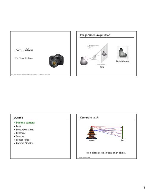
Image/Video Acquisition
Camera trial #1
source: Yung-Yu Chuang
Film
Digital Camera
scene film
Put a piece of film in front of an object.
1

Pinhole camera
pinhole camera
scene barrier
film
Add a barrier to block off most of the rays
• It reduces blurring
• The pinhole is known as the aperture
• The image is inverted
The Pinhole Camera Model (where)
(X,Y,Z)
d – focal length
y p
(x,y)
x p
d
⎛X
⎞
⎛ x⎞
⎛1
0 0 0⎞⎜
⎟
⎜ ⎟ ⎜
⎟⎜
Y ⎟
⎜ y⎟
= ⎜0
1 0 0⎟⎜
⎟
⎜ ⎟ ⎜
⎟ Z
⎝w⎠
⎝0
0 −1
d 0⎠
⎜
⎟
⎝ 1 ⎠
Y
center of
projection
(pinhole)
X
Z
Shrinking the aperture
Why not making the aperture as small as possible?
• Less light gets through
• Diffraction effect
2

Shrinking the aperture
Sharpest image is obtained when:
pinhole diameter
Example: If
f’ = 50mm,
λ
= 600nm (red),
d = 0.36mm
d = 2 f ' λ
Pinhole Images Outline
Exposure 4 seconds Exposure 96 minutes
Images copyright © 2000 Zero Image Co.
High-end commercial pinhole cameras
~$200
• Pinhole camera
• Lens
• Lens Aberrations
• Exposure
• Sensors
• Sensor Noise
• Camera Pipeline
3

Adding a lens
(Thin) Lens
scene film
Thin lens equation:
• Any object point satisfying this equation is in focus
Adding a lens
scene lens
film
A lens focuses light onto the film
“circle of
confusion”
• There is a specific distance at which objects are “in focus”
• Other points project to a “circle of confusion” in the image
Circle of Confusion
Circle of confusion proportional to the size of the aperture
4

Aperture controls Depth of Field
• Changing the aperture affects depth of field
– Smaller aperture:
• better DOF
• increased exposure
Thick Lens
• Corrects aberrations
• Change zoom
Depth of Field
Field of View (Zoom)
http://www.cambridgeincolour.com/tutorials/depth-of-field.htm
5

Field of View (Zoom) Simplified Zoom Lens in Operation
FOV depends of Focal Length
f
Smaller FOV = larger Focal Length
Outline
• Pinhole camera
• Lens
• Lens Aberrations
• Exposure
• Sensors
• Sensor Noise
• Camera Pipeline
From wikipedia
6

Radial Distortion
No distortion Pin cushion Barrel
• Radial distortion of the image
– Caused by imperfect lenses
– Deviations are most noticeable for rays that pass
through the edge of the lens
Radial Distortions
No Distortion Barrel Distortion Pincushion Distortion
• Radial distance from Image Center:
r u = r d + k 1 r d 3
r u = undistorted radius
r d = distorted radius
Correcting radial distortion
from Helmut Dersch
Correcting Radial Distortions
Before After
http://www.grasshopperonline.com/barrel_distortion_correction_software.html
7

Correcting Radial Distortions - Video
Video courtesy of Vigilant Ltd.
Vignetting
Vignetting Chromatic Aberration
L3 L2 L1
• More light passes through lens L3 for scene point A than scene point B
• Results in spatially non-uniform brightness (in the periphery of the image)
A
B
photo by Robert Johnes
longitudinal chromatic aberration transverse chromatic aberration
(axial) (lateral)
8

Chromatic Aberration
longitudinal chromatic
aberration (axial)
Canon EF 85/1.2 L USM
transverse chromatic
aberration (lateral)
Cosina 3.5-4.5/19-35
@ 20 mm
Good lens
Carl Zeiss Distagon
2.8/21
http://www.vanwalree.com/optics/chromatic.html
Chromatic Aberration
Spherical aberration Spherical aberration
• Rays parallel to the axis do not converge
• Outer portions of the lens yield smaller focal lengths
Near Lens Center Near Lens Outer Edge
Spherical lens are free of chromatic aberration but do not focus well.
Parabolic lens does.
9

Astigmatism
Different focal length for inclined rays
Lens Glare
• Stray inter-reflections of light within the optical lens system
• Happens when very bright sources are present in the scene
Reading: http://www.dpreview.com
Coma
point off the axis depicted as comet shaped blob
Outline
• Pinhole camera
• Lens
• Lens Aberrations
• Exposure
• Sensors
• Sensor Noise
• Camera Pipeline
10

Exposure
• Two main parameters:
– Aperture (in f stop)
– Shutter speed (in fraction of a second)
Aperture
• Aperture is the diameter of the lens opening,
usually specified by f-stop, f/D, a fraction of the
focal length.
– f/2.0 on a 50mm means that the aperture is 25mm
– f/2.0 on a 100mm means that the aperture is 50mm
• When a change in f-stop
occurs, the light is either
doubled or cut in half.
• Lower f-stop, more light
(larger lens opening)
• Higher f-stop, less light
(smaller lens opening)
Types of Shutters Leaf Shutter
• Advantages
– Uniform illumination
– Entire frame illuminated at once
• Disadvantages
– Illumination not constant over time
– Limitations on shutter speed
11

Focal Plane Shutter
Aperture vs. Shutter
• Advantages
– Cost effective (one shutter needed
for all lenses
– Can achieve very fast shutter speeds
(~1/10000 sec)
• Disadvantages
– May cause time distortion
Depth of Field
f/22 f/4
Small Aperture Large Aperture
(Low speed) (High speed)
Shutter speed – Rule of Thumb
• Handheld camera: shutter speed = 1 / f
• Stabilized gear: 2-3 shutter speeds slower
– Optical image stabilization
• Canon - IS (Image Stabilizer) lenses
• Nikon - VR (Vibration Reduction) lenses
• Sigma - OS (Optical Stabilizer) lenses
– CCD-shift stabilization
• Konica Minolta’s Anti-Shake cameras
• Pentax’s Shake-Reduction cameras
Aperture vs. Shutter
1/30 sec. @ f/22
Motion Blur
1/6400 sec. @ f/2.5
Small Aperture Large Aperture
(Low speed) (High speed)
12

High Dynamic Range Image Short exposure
Long exposure
Real world
radiance
Picture
intensity
10 -6 10 6
dynamic range
10 -6 10 6
Pixel value 0 to 255
Real world
radiance
Picture
intensity
10 -6 10 6
dynamic range
10 -6 10 6
Pixel value 0 to 255
Varying shutter speeds
13

HDR – High Dynamic Range Outline
Spatial Sampling
• When a continuous scene is imaged on the
sensor, the continuous image is divided into
discrete elements - picture elements (pixels)
• Pinhole camera
• Lens
• Lens Aberrations
• Exposure
• Sensors
• Sensor Noise
• Camera Pipeline
Spatial Sampling
14

Sampling
• The density of the sampling denotes the
separation capability of the resulting image
• Image resolution defines the finest details that
are still visible by the image
• We use a cyclic pattern to test the separation
capability of an image
0
Sampling Frequency
x
Sampling Frequency
Nyquist Frequency
• Nyquist Rule: To observe details at frequency f
(wavelength d) one must sample at frequency > 2f
(sampling intervals < d/2)
•
• The Frequency 2f is the NYQUIST frequency.
• Aliasing: If the pattern wavelength is less than 2d
erroneous patterns may be produced.
1D Example:
0
15

Aliasing - Moiré Patterns Quantization
Digitizers (Quantization)
Image Sensors
• Considerations
• Speed
• Resolution
• Signal / Noise Ratio
• Cost
16

MOS (Metal Oxide Semiconductor)
• Photosensitive element
• Charge acquired depends on the number of
photons which reach the element
• CCD devices are arrays of this basic element
CCD (Charge Coupled Device)
• Boyle and Smith, 1969, Bell Labs
• Converts light into electrical signal (pixels)
Photoelectric Effect
Increasing energy
Conduction Band
Valence Band
1.26eV
Hole Electron
• Thermally generated electrons are indistinguishable
from photo-generated electrons � ‘Dark Current’.
CCD Readout
Bucket Brigade
• Integration
• Charge Shift and
Read-out
•Charge Amplifier
17

CMOS (Complementary Metal-Oxide Semiconductor)
• Each pixel owns its own charge-voltage conversion
• No need for external shutter (electronic shutter)
• The chip outputs digital bits
• Much faster than CCD devices
CCD vs. CMOS
• Mature technology
• Specific technology
• High production cost
• High power consumption
• Higher fill factor
• Blooming
• Sequential readout
Spectral Response of a Typical CCD Sensitivity
• Sensitivity
Reset
Output
T int
∆V
• Recent technology
• Standard IC technology
• Cheap
• Low power
• Less sensitive
• Per pixel amplification
• Random pixel access
• Smart pixels
• On chip integration
with other components
– is the ratio of voltage response to the photo energy illuminated.
Voltage Drop (V/s)
Slope = sensitivity
( V / lx-s)
Light intensity (lx)
18

Sensor Size Comparison Sensor Parameters
Fill Factor
• The ratio between the light sensitive pixel area
and the total pixel area.
Total pixel area:
5µm x 5µm
Fill factor ≈ 40%
Photo
Sensing
Area
• Fill factor
– The area in the sensor that is truly sensitive to light
– Shift registers and others can reduce it up to a 30%
• Well capacity
– The quantity of charge that can be stored in each pixel
– Close relation with pixel dimensions
• Integration time:
– Exposure time that is required to excite the CCD elements
– IDepends on the scene brightness
• Acquisition time:
– Time needed to transfer the information gathered by the CCD
– Depends on the number of pixels in the sensor
Outline
• Pinhole camera
• Lens
• Lens Aberrations
• Exposure
• Sensors
• Sensor Noise
• Camera Pipeline
19

Sensor noise
Noise Sources
• Photon noise / Shot Noise (Poisson)
• Dark Noise (Constant)
•Thermal noise (Poisson)
• Resetting (fixed)
• Read-out noise (white & 1/f)
• Blooming
Poisson Distribution, FT = 5
0 .2
0 . 1 5
0 .1
0 . 0 5
(After T. Lomheim, The Aerospace Corporation)
http://www.stw.tu-ilmenau.de/~ff/beruf_cc/cmos/cmos_noise.pdf
0
0 2 0 4 0 6 0 8 0 1 0 0
Poisson Distribution : std equals sqrt of Mean.
σ
2
shot
N
= FT =
N
photons
Photon Shot Noise
• Light is quantum in nature
• Noise due to statistics of the detected photons
themselves
• The probability distribution for N photons to be
counted in an observation time T is Poisson
P
( N | F,
T )
( FT )
N −FT
e
N!
• F = fixed average flux (photons/sec)
Poisson Distribution, FT = 10
0 . 1 4
0 . 1 2
0 .1
0 . 0 8
0 . 0 6
0 . 0 4
0 . 0 2
=
0
0 2 0 4 0 6 0 8 0 1 0 0
N
20

Poisson Distribution, FT = 20
0 .1
0 . 0 8
0 . 0 6
0 . 0 4
0 . 0 2
0
0 2 0 4 0 6 0 8 0 1 0 0
Photon Noise
• More noise in bright parts of the image
• You can identify the white and black regions from
the noise image
N
Poisson Distribution, FT = 50
0 . 0 6
0 . 0 5
0 . 0 4
0 . 0 3
0 . 0 2
0 . 0 1
0
0 2 0 4 0 6 0 8 0 1 0 0
N
• As FT grows, Poisson distribution approaches Gaussian
distribution
• Signal To Noise (SNR) Increases with Mean.
2 2
N N
SNR = = = N
2
σ N
Photon Noise
Photon Noise more noticeable in dark images.
21

Dark Current Noise
• Electron emission when no light
• Dark current noise is high for long exposures
• To remove (some) of it
– Calibrate the camera (make response linear)
– Capture the image of the scene as usual
– Cover the lens with the lens cap and take another
picture
– Subtract the second image from the first image
Quantum Efficiency
• Not every photon hitting a pixel creates a free electron
• Quantum Efficiency (QE) =
– electrons collected / photons hitting the pixel
QE [%]
• QE heavily depends on the
wavelength
• QE < 100% degrades the SNR of a camera
SNR =
e
QE SNR
p
blue � green � red
• Typical max QE values : 25% (CMOS) … 60% (CCD)
lambda [nm]
Dark Current Noise
Original image + Dark Current Noise Image with lens cap on
Sensor noise
ideal relationship between
electrons and impinging photons
Light Signal (QE = 50)
Result of subtraction
CCD capacity limit
Photon Noise affects (QE = 50)
Copyright Timo Autiokari,
22

Outline
• Pinhole camera
• Lens
• Lens Aberrations
• Exposure
• Sensors
• Sensor Noise
• Camera Pipeline
Sensor Response
• The response of a sensor is proportional to the
radiance and the throughput
Camera pipeline
Measurement Equation
• Scene Radiance L(x,ω,t,λ)
• Optics (x’,ω’) = T(x,ω,λ)
• Pixel Response P(x,λ)
• Shutter S(x,ω,t)
23

SLR (Single-Lens Reflex)
• Reflex (R in SLR) means that we see through
the same lens used to take the image.
• Not the case for compact cameras
Camera calibration
• Geometric
– How pixel coordinates relate to directions in
the world
• Photometric
– How pixel values relate to radiance amounts
in the world
SLR view finder
Mirror
(flipped for exposure)
Light from scene
lens
Prism
Mirror
(when viewing)
Color Chart Calibration
Your eye
Film/sensor
• Important preprocessing step for many vision and graphics
algorithms
• Use a color chart with precisely known reflectance
90%
59.1% 36.2% 19.8% 9.0%
3.1%
0
0 ? 1
Irradiance = const * Reflectance
• Use more camera exposures to fill up the curve
• Method assumes constant lighting on all patches and works best
when source is far away
• Unique inverse exists because g is monotonic and smooth
Pixel Values
255
g
−1
g
?
24

Space of response curves Sensing Color
Multi-Chip
wavelength
dependent
light
3 CCD
beam splitter
Field Sequential
Foveon X3 TM
Bayer pattern
25

Field Sequential Field Sequential
Embedded color filters
Color filters can be manufactured directly onto
the photodetectors.
Color filter array
Bayer pattern
Color filter arrays (CFAs)/color filter mosaics
26

Color filter array
Kodak DCS620x
Color filter arrays (CFAs)/color filter mosaics
Bayer’s pattern
Demosaicking CFA’s Color filter array
red green blue output
27

X3 technology
red green blue output
Cameras with X3
Sigma SD10, SD9 Polaroid X530
Hanvision HVDUO
5M/10M
Foveon X3 sensor
Bayer CFA
Color processing
X3 sensor
• After color values are recorded, more color
processing usually happens:
– White balance
– Non-linearity to approximate film response or match
TV monitor gamma
28

White Balance
warmer +3
Gamma Correction
automatic white balance
• Gamma correction applied by the converter
redistributes the pixel luminance values so that
limited brightness range captured by the sensor
is “mapped” to match our eye’s sensitivity.
Gamma = 2.2 is a good match to distribute
relative brightness in a print or in a video
display.
Manual white balance
white balance with
the white book
white balance with
the red book
Gamma =1 vs. Gamma = 2.2
29

Many Sources for Degradation
• Sampling in space
Pixels
• Sampling in intensity
Quantization
• Sampling in color
Color Filter Array (CFA)
• Sampling in time
Exposure, Interlacing
• Sampling in frequency
Lens and pixel PSF (point-spread-function)
30